Topological Charge in Two Flavors QCD with Optimal Domain-Wall Fermion

Abstract:

We measure the topological charge of the gauge configurations generated by lattice simulations of 2 flavors QCD on a $16^{3}\times 32$ lattice, with Optimal Domain-Wall Fermion (ODWF) at $N_{s}=16$ and plaquette gauge action at $\beta=5.90$. Using the Adaptive Thick-Restart Lanczos algorithm, we project the low-lying modes of the 4D effective Dirac operator of ODWF, and obtain the topological charge and topological susceptibility. Our result of topological susceptibility agrees with the sea-quark mass dependence predicted by the chiral perturbation theory, and provides a determination of the chiral condensate.

1 Introduction

In Quantum Chromodynamics (QCD), the topological susceptibility ($\chi_{t}$) is the most essential quantity to measure the topological charge fluctuation of the QCD vacuum, which plays an important role in breaking the $U_{A}(1)$ symmetry. Theoretically, $\chi_{t}$ is defined as

$$\chi_{t}=\int d^{4}x\left<\rho(x)\rho(0)\right>=\frac{\left<Q_{t}^{2}\right>}{\Omega}$$ (1)

where

$$\rho(x)=\frac{1}{32\pi^{2}}\epsilon_{\mu\nu\lambda\sigma}\mathrm{tr}[F_{\mu\nu}(x)F_{\lambda\sigma}(x)],\hskip 14.22636ptQ_{t}\equiv\int d^{4}x\rho(x),$$ (2)

$Q_{t}$ is the topological charge (which is an integer for QCD), $\rho(x)$ is the topological charge density, and $\Omega$ is the space-time volume. In the chiral perturbation theory (ChPT), the quark mass dependence of $\chi_{t}$ was derived at the tree level [1] in 1992, and it has been extended to the one-loop order recently [2]. For $N_{f}=2$, these ChPT formulas can be written as

$$\chi_{t}/m_{u} = \frac{\Sigma}{1+m_{u}/m_{d}},$$ (3)

$$\chi_{t}/m_{u} = \frac{\Sigma}{1+m_{u}/m_{d}}\left[1-\biggl{(}\frac{3M_{\pi}^{2}}{32\pi^{2}F_{\pi}^{2}}\biggr{)}\ln\frac{M_{\pi}^{2}}{\mu^{2}_{sub}}+K_{6}(m_{u}+m_{d})+2(2K_{7}+K_{8})\frac{m_{u}m_{d}}{m_{u}+m_{d}}\right],$$ (4)

where $\Sigma$ is the chiral condensate, $F_{\pi}$ the pion decay constant, and $K_{i}$ are related to low energy constants $L_{i}$. A salient feature of $\chi_{t}$ is that it is suppressed in the chiral limit ($m_{u}\rightarrow 0$) due to the internal quark loops. Most importantly, (3) and (4) provide a viable way to extract $\Sigma$ and other low energy constants.

However, one cannot determine $Q_{t}$ reliably using the link variables, due to the rather strong fluctuations at short distances. Instead, we consider the Atiyah-Singer index theorem [3]

$$Q_{t}=n_{+}-n_{-}=\mbox{index}({\cal D}),$$ (5)

where $n_{\pm}$ is the number of zero modes of the massless Dirac operator ${\cal D}\equiv\gamma_{\mu}(\partial_{\mu}+igA_{\mu})$ with $\pm$ chirality. Thus, by couting the zero modes of the massless Dirac operator, we can determine $Q_{t}$ and $\chi_{t}$ for an ensemble of gauge configurations.

Recently, the topological susceptibility has been measured in unquenched lattice QCD with exact chiral symmetry, for $N_{f}=2$ lattice QCD with overlap fermion in a fixed topology [4], and $N_{f}=2+1$ lattice QCD with domain-wall fermion [5]. These results are in good agreement with the ChPT at the tree level (3).

In this work, we measure the topological charge of the gauge configurations generated by lattice simulations of 2 flavors QCD on a $16^{3}\times 32$ lattice, with the Optimal Domain-Wall Fermion (ODWF) [6] at $N_{s}=16$, and plaquette gauge action at $\beta=5.90$. Mathematically, ODWF is a theoretical framework which can preserve the chiral symmetry optimally for any finite $N_{s}$. Thus the artifacts due to the chiral symmetry breaking with finite $N_{s}$ can be reduced to the minimum, especially in the chiral regime. The 4D effective operator of massless ODWF is

$$D=m_{0}[1+\gamma_{5}S_{opt}(H_{w})],\quad S_{opt}(H_{w})=\frac{1-\prod_{s=1}^{N_{s}}T_{s}}{1+\prod_{s=1}^{N_{s}}T_{s}},\quad T_{s}=\frac{1-\omega_{s}H_{w}}{1+\omega_{s}H_{w}},$$ (6)

which is exactly equal to the Zolotarev optimal rational approximation of the overlap Dirac operator [7]. That is, $S_{opt}(H_{w})=H_{w}R_{Z}(H_{w})$, where $R_{Z}(H_{w})$ is the optimal rational approximation of $(H_{w}^{2})^{-1/2}$ [8].

We outline our scheme of projecting the low-lying eigenmodes of $D$ as follows. Using $[DD^{\dagger},\gamma_{5}]=0$, and the representation

$$D\left|\theta\right>=\lambda(\theta)\left|\theta\right>,\hskip 28.45274pt\lambda(\theta)=m_{0}(1+e^{i\theta}),$$ (7)

we obtain

$$S_{\pm}\left|\theta\right>_{\pm}\equiv P_{\pm}H_{w}R_{Z}(H_{w})P_{\pm}\left|\theta\right>_{\pm}=\pm\cos\theta\left|\theta\right>_{\pm},\quad P_{\pm}=\frac{1\pm\gamma_{5}}{2},$$ (8)

where $\left|\theta\right>=P_{+}\left|\theta\right>+P_{-}\left|\theta\right>=\left|\theta\right>_{+}+\left|\theta\right>_{-}$. Thus, we can perform the eigenmode projection on the operator $S_{\pm}$ instead of $D$. Moreover, $\left|\theta\right>_{\pm}$ are related to each other through the relation

$$\left|\theta\right>=\frac{1}{i\sin\theta}(\gamma_{5}S-e^{-i\theta})\left|\theta\right>_{\pm},\hskip 28.45274pt\theta\neq 0,\pm\pi,\pm 2\pi,\ldots$$ (9)

Assuming the zero modes only residing in either $+$ or $-$ chirality, we project the low-lying modes of $D$ as follows. First, we project the smallest eigenmodes of $S_{+}$. If $D$ has zero modes with positive chirality, then the smallest eigenvalues of $S_{+}$ are equal to $-1$, and the corresponding full eigenvectors can be obtained using Eq. (9). Otherwise, we have to check whether $D$ has zero modes with negative chirality by projecting the largest eigenmodes of $S_{-}$. If $D$ has zero modes with negative chirality, the largest eigenvalues of $S_{-}$ are equal to $+1$, and the corresponding full eigenvectors can be obtained using Eq. (9). Finally, for non-zero low-lying eigenmodes, we can pick either $+$ or $-$ chirality of Eq. (8) for projection, then obtain the full eigenvectors using Eq. (9).

2 The TRLan algorithm

In general, the low-mode projection of a large sparse matrix $A$ can be carried out via iterative process, such as the Lanczos algorithm or the Arnoldi algorithm. The common procedure is to construct an orthonormal basis from the Krylov subspace starting from an initial vector $r_{0}$,

$$\mathcal{K}(A,r_{0})={\mathrm{s}pan}\left\{r_{0},\,Ar_{0},\,A^{2}r_{0},\ldots,\,A^{m-1}r_{0}\right\}.$$ (10)

The linear combinations of $\{A^{i}r_{0},i=0,1,\ldots m-1\}$ form the Ritz vectors of $A$, which converge to the eigenvectors of $A$ as $m$ becomes very large.

Input: $r_{0}$, $\beta_{0}=||r_{0}||$, $q_{0}=0$ For: $i$ = 1, 2, … • $q_{i}=r_{i-1}/\beta_{i-1}$ • $p=Aq_{i}$ • $\alpha_{i}=q_{i}^{\dagger}p$ • $r_{i}=p-\alpha_{i}q_{i}-\beta_{i-1}q_{i-1}$ • $\beta_{i}=||r_{i}||$
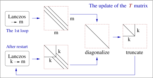
(a)	(b)

Figure 1: (a) The basic Lanczos process; (b) The Lanczos algorithm with Thick-Restart.

Since $H_{w}$ and $S_{\pm}$ are Hermitian matrices, it is natural to use the Lanczos algorithm. The basic Lanczos process (see Fig.1-(a)) is to construct the following factorization

$$AQ_{m}=Q_{m}T_{m}+\beta_{m}q_{m+1}e_{m}^{T},$$ (11)

where $\{q_{1}$, $q_{2}$, …, $q_{m}\}$ form an orthonormal basis, $Q_{m}=[q_{1},q_{2},\ldots,q_{m}]$, $e_{m}$ is the $m$-th column of the $m\times m$ identity matrix, and $T_{m}$ is a tridiagonal matrix with diagonal elements $\alpha_{i}$ and sub-diagonal elements $\beta_{i}$. Then the Ritz pairs $(\hat{\lambda}_{i},\hat{x}_{i})$ can be obtained from

$$\hat{T}_{m}=U^{\dagger}_{m}T_{m}U_{m},\hskip 28.45274ptX_{m}=Q_{m}U_{m},$$ (12)

where $\hat{T}_{m}$ is diagonal with eigenvalues $\hat{\lambda}_{i}$, $U_{m}$ is a unitary matrix, and $X_{m}=[\hat{x}_{1},\hat{x}_{2},\ldots,\hat{x}_{m}]$. As $m$ becomes very large, the Ritz pairs $(\hat{\lambda}_{i},\hat{x}_{i})$ converge to the eigenmodes $(\lambda_{i},x_{i})$ of $A$.

However, the Lanczos algorithm suffers from the following problems. Some specious Ritz values may repeatedly appear when $m$ goes to larger values. This is due to the fact that the vectors $\{q_{i}\}$ lose orthogonality rapidly in the finite precision arithmatics. Hence one has to apply the Gram-Schmidt procedure to re-orthogonalize them during the iteration. Also, it requires a large number of $q_{i}$ to project a few Ritz pairs, consuming a large amount of memory and slowing down the computation. A way to overcome these problems is to perform a restart.

There are several restart schemes, in which the Thick-Restart Lanczos algorithm (TRLan) [9] turns out to be the most efficient for our purpose. The TRLan algorithm is illustrated in Fig.1-(b), where the squares in the diagram stand for the square matrix $T_{m}$, in which the non-zero matrix elements are denoted by black lines.

	$H_{w}$: $k^{\prime}=240$, $m=340$				$S_{+}$: $k^{\prime}=100$, $m=200$, $n_{p}=240$
method	N_restarts	# of $A\cdot v$	time(s)	speed up	N_restarts	# of $A\cdot v$	time(s)	speed up
ARPACK	388	35390	136460	1.00	13	1050	112632	1.00
TRLan	999	100140	572951	0.24	12	1300	105790	1.06
$\nu$-TRLan	383	59145	78058	1.75	11	1030	90496	1.24

Table 1: The benchmark of low-mode projection of $H_{w}$ and $S_{+}$ for a non-trivial gauge configuration ($Q_{t}=3$) at $\beta=5.9$ and $m_{q}a=0.01$. Here $k^{\prime}$ is the number of low-modes projected, $m$ is the dimension of Krylov subspace, and $n_{p}$ is the number of low-modes of $H_{w}$ used for low-mode preconditioning in the projection of the low-modes of $S_{+}$.

Obviously, the performance of the TRLan algorithem depends on the truncated dimension $k$ and the dimension $m$ of the Krylov subspace. Now the question is what is the optimal value of $k$ (for a given $m$) such that for each restart, the reduction factor $d_{j}$ of the residual of the $j$-th (not converged) Ritz pair is maximized, while the number of floating-point operations (FPOs) is minimized. In other words, at each restart, we try to find the optimal $k$ by maximizing the object function [10]

$$f(k)=\frac{d_{j}}{\mathrm{\#\ of\ FPOs}},\hskip 14.22636ptd_{j}\simeq\mathcal{C}_{m-k}(1+2\gamma),\hskip 14.22636pt\gamma=\frac{\hat{\lambda}_{k+1}-\hat{\lambda}_{j}}{\hat{\lambda}_{m}-\hat{\lambda}_{k+1}},$$ (13)

where $\mathcal{C}_{m-k}(z)$ is the Chebyshev polynomial of degree $m-k$. For the number of FPOs, we only count the dominant parts which are directly related to the dimension $m$, namely, the re-orthogonalization and the update of Ritz vectors. This modified algorithm is called the Adaptive Thick-Restart Lanczos algorithm, which can attain substantial performance gain, with faster convergence and fewer FPOs.

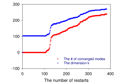
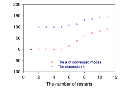
(a)	(b)

Figure 2: The number of converged Ritz pairs and the dimension $k$ versus the number of restarts for the $\nu$-TRLan algorithm: (a) $H_{w}$ ($m=340$); (b) $S_{+}$ of the overlap operator ($m=240$).

For benchmarking, we project the low-lying eigenmodes of $H_{w}$ and $S_{+}$, using a nontrivial configuration ($Q_{t}=3$) generated by the 2-flavor QCD simulation on a $16^{3}\times 32$ lattice, with ODWF fermion at $N_{s}=16$ and $m_{sea}a=0.01$, and the plaquette gauge action at $\beta=5.90$. In Table 1, we present our benchmark results for three different methods: ARPACK (Arnoldi algorithm with Implicit Restart), TRLan (Thick-Restart Lanczos), and $\nu$-TRLan (Adaptive Thick-Restart Lanczos). For TRLan (by definition $k=k^{\prime}$, where $k^{\prime}$ is the number of low-modes we want to project, and $k$ is the truncated dimension at each restart), we see that its rate of convergence tends to be very slow for $H_{w}$, with a rather large condition number ($\sim 10^{6}$). On the other hand, for $\nu$-TRLan, $k$ is automatically adjusted to be an optimal value in each restart ($k^{\prime}<k<m$, see Fig. 2), thus the rate of convergence is dramatically improved. It turns out that, for both $H_{w}$ and $S_{\pm}$, $\nu$-TRLan is faster than TRLan and ARPACK. Therefore, we use $\nu$-TRLan to project the low-lying eigenmodes of $H_{w}$ and $D$.

3 Lattice setup

Simulations are carried out for two flavors ($N_{f}=2$) QCD on a $16^{3}\times 32$ lattice at a lattice spacing $a\sim$ 0.11 fm, for eight sea quark masses in the range $m_{q}a=0.01,0.02,\cdots,0.08$ [11]. For the gluon part, the plaquette action is used at $\beta$ = 5.90. For the quark part, the optimal domain-wall fermion is used with $N_{s}=16$. After discarding 300 trajectories for thermalization, we accumulated $3000-3200$ trajectories in total for each sea quark mass. From the saturation of the binning error of the plaquette, as well as the evolution of the topological charge, we estimate the autocorrelation time to be around 10 trajectories. Thus we sample one configuration every 10 trajectories, then we have $270-290$ configurations for each sea quark mass.

For each configuration, we calculate the zero modes and 80 conjugate pairs of the lowest-lying eignmodes of the overlap Dirac operator. We outline our procedures as follows. First, we project 240 low-lying eigenmodes of $H_{w}^{2}$ using $\nu$-TRLan alogorithm, where each eigenmode has a residual less than $10^{-12}$. Then we approximate the sign function of the overlap operator by the Zolotarev optimal rational approximation with 64 poles, where the coefficents are fixed with $\lambda_{max}^{2}=(6.4)^{2}$, and $\lambda_{min}^{2}$ equal to the maximum of the 240 projected eigenvalues of $H_{w}^{2}$. Then the sign function error is less than $10^{-14}$. Using the 240 low-modes of $H_{w}^{2}$ and the Zolotarev approximation with 64 poles, we project the zero modes plus 80 conjugate pairs of of the lowest-lying eignmodes of the overlap operator with the $\nu$-TRLan algorithm, where each eigenmode has a residual less than $10^{-12}$.

4 Results

In Fig. 3, we plot the topological susceptibility $\chi_{t}=\left<(Q_{t}-\left<Q_{t}\right>)^{2}\right>/\Omega$ as a function of the sea quark mass $m_{q}$. For all eight sea quark masses, our data are well fitted by a linear function $F+Gm_{q}$ with the intercept $F=0.47(2.37)\times 10^{-5}$ and the slope $G=5.50(4)\times 10^{-3}$. Evidently, the intercept is consistent with zero, in agreement with the $\chi$PT expectation (3). Equating the slope to $\Sigma/N_{f}$, we obtain $\Sigma=0.0110(7)$. In order to convert $\Sigma$ to that in the $\overline{\mathrm{MS}}$ scheme, we calculate the renormalization factor $Z_{m}^{\overline{\mathrm{MS}}}(\mathrm{2~{}GeV})$ using the non-perturbative renormalization technique through the RI/MOM scheme [12], and obtain $Z_{m}^{\overline{{\mathrm{MS}}}}(\mbox{2~{}GeV})=0.5934(10)$ [13]. Then the value of $\Sigma$ is transcribed to

$$\Sigma^{\overline{{\mathrm{MS}}}}(\mathrm{2~{}GeV})=[\mathrm{261(5)(7)~{}MeV}]^{3},$$ (14)

which is in agreement with our previous results : $\Sigma^{\overline{\mathrm{MS}}}(\mathrm{2~{}GeV})=[\mathrm{245(5)(12)~{}MeV}]^{3}$ for $N_{f}=2$ lattice QCD with overlap fermion in a fixed topology [4], and $\Sigma^{\overline{\mathrm{MS}}}(\mathrm{2~{}GeV})=[\mathrm{253(4)(6)~{}MeV}]^{3}$ for $N_{f}=2+1$ lattice QCD with domain-wall fermion [5]. The statistical error represents a combined error (including those due to $a^{-1}$ and $Z_{m}^{\overline{\mathrm{MS}}}$). The systematic error is estimated from the turncation of higher order effects and the uncertainty in the determination of lattice spacing with $r_{0}=0.49$ fm. Since our calculation is done at a single lattice spacing, the discretization error cannot be quantified reliably, but we do not expect much larger error because our lattice action is free from $O(a)$ discretization effects.

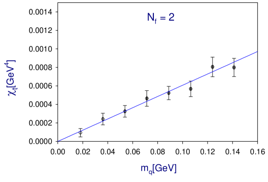
Figure 3: The topological susceptibility of two-flavors QCD with the optimal domain-wall fermion.

5 Concluding remarks

We have measured the topological charge of the gauge configurations generated by lattice simulations of 2 flavors QCD on a $16^{3}\times 32$ lattice, with Optimal Domain-Wall Fermion (ODWF) at $N_{s}=16$ and plaquette gauge action at $\beta=5.90$. We use the Adaptive Thick-Restart Lanczos algorithm to compute the low-lying eigenmodes of $H_{w}^{2}$ and the overlap Dirac operator. Our result of $\chi_{t}$ agrees with the sea-quark mass dependence predicted by the ChPT at the tree level, and provides a good determination of the chiral condensate. Furthermore, our result of $\chi_{t}$ also agrees with the the NLO ChPT, Eq. (4). We will present the details in a forthcoming paper [14].

- [1] H. Leutwyler and A. Smilga, Phys. Rev. D 46, 5607 (1992).
- [2] Y. Y. Mao and T. W. Chiu [TWQCD Collaboration], Phys. Rev. D 80, 034502 (2009)
- [3] M. F. Atiyah and I. M. Singer, Annals Math. 87, 484 (1968).
- [4] S. Aoki et al. [JLQCD and TWQCD Collaborations], Phys. Lett. B 665, 294 (2008)
- [5] T. W. Chiu, T. H. Hsieh and P. K. Tseng [TWQCD Collaboration], Phys. Lett. B 671, 135 (2009)
- [6] T. W. Chiu, Phys. Rev. Lett. 90, 071601 (2003); Nucl. Phys. Proc. Suppl. 129, 135 (2004)
- [7] H. Neuberger, Phys. Lett. B 417, 141 (1998); R. Narayanan and H. Neuberger, Nucl. Phys. B 443, 305 (1995)
- [8] T. W. Chiu, T. H. Hsieh, C. H. Huang and T. R. Huang, Phys. Rev. D 66, 114502 (2002)
- [9] K. Wu and H. Simon, SIAM J. Matrix Anal. Appl. 22, 602, 2000.
- [10] I. Yamazaki, Z. Bai, H. Simon, L.W. Wang, and K. Wu, Tech. Rep. LBNL-1059E (2008).
- [11] T. W. Chiu et al. [TWQCD Collaboration], PoS LAT2009, 034 (2009) [arXiv:0911.5029 [hep-lat]]; PoS LAT2010, 099 (2010)
- [12] G. Martinelli, C. Pittori, C. T. Sachrajda, M. Testa and A. Vladikas, Nucl. Phys. B 445, 81 (1995)
- [13] T.W. Chiu et al. [TWQCD Collaboration], in preparation.
- [14] T.W. Chiu, T.H. Hsieh, Y.Y. Mao [TWQCD Collaboration], in preparation.