Yet Another Riemann Hypothesis

Abstract

This short note presents a peculiar generalization of the Riemann hypothesis, as the action of the permutation group on the elements of continued fractions. The problem is difficult to attack through traditional analytic techniques, and thus this note focuses on providing a numerical survey. These results indicate a broad class of previously unexamined functions may obey the Riemann hypothesis in general, and even share the non-trivial zeros in particular.

1 Introduction

The Riemann zeta can be expressed as an integral in the following form[1]:

$$\zeta(s)=\frac{s}{s-1}-s\int_{0}^{1}h(x)x^{s-1}dx$$

where

$$h(x)=\frac{1}{x}-\left\lfloor\frac{1}{x}\right\rfloor$$

is sometimes called the Gauss map. Here, $\left\lfloor y\right\rfloor$ is the largest integer less than or equal to $y$. The Gauss map lops of a digit in the continued fraction expansion of $x$. If one writes the continued fraction expansion[2] of $0<x\leq 1$ as

$$x=[a_{1},a_{2},a_{3},\cdots]=\frac{1}{a_{1}+\frac{1}{a_{2}+\frac{1}{a_{3}+\ldots}}}$$

then $h(x)=[a_{2},a_{3},\cdots]$. It is a (reverse) shift operator on the continued fraction expansion. The study of continued fractions is interesting because of their proximity to various problems of fractals and dynamical systems, including ties to Farey fractions, the modular group via the Cantor set, and the Minkowski question mark function. More immediately, the transfer (Ruelle-Frobenius-Perron) operator of the Gauss map is the Gauss-Kuzmin-Wirsing operator, which has a number of interesting properties of its own.

In this note, we observe that the Gauss map can also be thought of as one particular element of the permutation group acting on an infinite dimensional representation of the real numbers. Thus, we are lead to contemplate other elements of the permutation group. Specifically, consider the permutation operator

$$S_{p,q}:[a_{1},\cdots,a_{p},\cdots,a_{q},\cdots]\mapsto[a_{1},\cdots,a_{q},\cdots,a_{p},\cdots]$$ (1)

which exchanges the $p$’th and $q$’th digits of the continued fraction expansion of $x$. Note that $S_{p,q}$ maps the unit interval onto the unit interval, and is discontinuous at a countably infinite number of points. The generalized Riemann hypothesis that we choose to explore concerns the zeros of the integral

$$\zeta_{p,q}(s)=\frac{s}{s-1}-s\int_{0}^{1}S_{p,q}(x)x^{s-1}dx$$ (2)

That is, is it possible that the (non-trivial) zeros of $\zeta_{p,q}(s)$ all lie on the $\Re s=\frac{1}{2}$ axis? This text is devoted to the exploration of this possibility.

This integral can be evaluated, but only with considerable difficulty. The function $S_{p,q}\left(x\right)$ is a piece-wise combination of unimodular Mobius functions, that is, a piece-wise collection of

$$\frac{ax+b}{cx+d}$$

with integer values of $a$, $b$, $c$ and $d$, such that $ad-bc=\pm 1$. This structure follows from the general theory of continued fractions[2]. Section 3 below provides a set of graphs visualizing $S_{p,q}(x)$, showing their piece-wise nature. The functions are clearly “fractal” or self-similar; a general discussion of the self-similarity is given in [4]. Because of the piece-wise structure, the integral can be evaluated analytically. The result is a messy set of nested sums that don’t seem to provide any particular insight. One might expect that these sums would simplify, or at least, speed up numeric evaluation, but they don’t even seem very useful for that. Details are given in section 5.

It is easiest, at first, to perform the integration numerically. Treating the integral as a very simple Newtonian integration sum with equally spaced abscissas, one gets:

$$\zeta_{N;p,q}\left(s\right)=\frac{s}{s-1}-\frac{s}{N}\;\sum_{n=0}^{N-1}S_{p,q}\left(\frac{2n+1}{2N}\right)\;\left(\frac{2n+1}{2N}\right)^{s-1}$$ (3)

This summation converges very slowly and very noisily as $N\to\infty$ but a numerical evaluation for large $N$ can give some basic insight. First and foremost, one discovers that, at least qualitatively, the sums $\zeta_{N;p,q}\left(s\right)$ behave very much like the corresponding sum for the Riemann zeta. This provides the simplest evidence in support of the hypothesis. A graphical visualization is provided in section 3.

2 Continued Fractions; Permutation Groups

Continued fractions provide a representation of the real numbers in the infinite Cartesian product space $\mathbb{M}^{\omega}=\mathbb{M\times M\times}...$ where $\mathbb{M}=\mathbb{N}\cup\{\infty\}$ and $\mathbb{N}=\mathbb{Z}^{+}$ is the set of positive integers. The continued fraction brackets are a function that maps this product space to the real numbers, i.e. $[\,]:\mathbb{N}^{\omega}\mathbb{\rightarrow R}$. The mapping is, strictly-speaking, surjective, yet, in a certain sense, is “almost everywhere” bijective. That is, every non-rational real number corresponds to a unique continued fraction; only the rationals have multiple expansions.

The above definition of a continued fraction differs slightly from the conventional norm. Usually, continued fractions are considered to be of finite length for the rationals, and infinite-length for the non-rational reals. This can create confusion when discussing $S_{p,q}(x)$ when either $p$ or $q$ are larger than the length of the continued fraction. The trick of adjoining infinity to the naturals is the most straight-forward way of avoiding this problem. The cost of this trick is that a “very large part” of the Cartesian product maps to the rationals. Thus, for example, the continued fraction expansion for 0 is $0=[\infty,a_{2},a_{3},...]$ for any arbitrary positive integers $a_{k}$. All rationals suffer in the same way: a finite continued fraction is just one where $\infty$ appears somewhere in the expansion, i.e. $[a_{1},a_{2},...,a_{N}]=[a_{1},a_{2},...,a_{N},\infty,a_{N+2},...]$. This can be papered over by considering the reals as the quotient space of sequences modulo the kernel of $[\,]$. That is, define a quotient space $\mathbb{S}=\mathbb{M}^{\omega}/\ker[\,]$, so that the operator $[\,]:\mathbb{S}\to\mathbb{R}$ is 1-1 and onto in this quotient space. Since this map is bijective, it is invertible, and thus, any function on the reals $\mathbb{R}$ and be expressed as an equivalent function on $\mathbb{S}$, and vice-versa: functions on the sequence space $\mathbb{M}^{\omega}$ correspond to functions on the reals.

Elements of the (infinite-dimensional) permutation group acting on $\mathbb{S}$ are given by equation 1. The $S_{p,q}(x)$ are discontinuous, but only on a countable set of points. That is, for fixed $p,q,$ the function $S_{p,q}(x)$ is discontinuous on the proverbial ”set of measure zero”, and so one can easily form well-defined integrals using ordinary techniques.

3 Structural overview

A graphical presentation of the functions $S_{1,2}\left(x\right)$, $S_{1,3}\left(x\right)$, $S_{1,4}\left(x\right)$ and $S_{2,3}\left(x\right)$ are shown in figure 1. The fractal, self-similar nature of these functions is readily apparent.

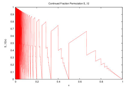
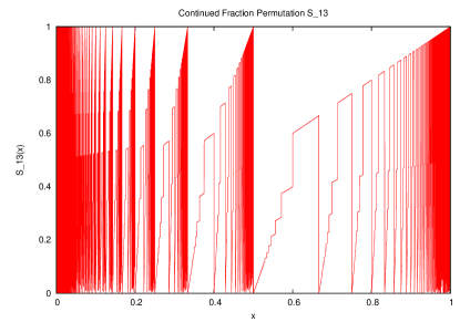
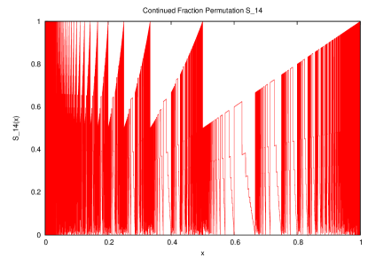
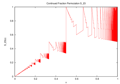
Figure 1: Continued Fraction Permutations

The above figures show a set of graphs for various continued fraction permutations $S_{p,q}(x)$ for the swap operator $S_{p,q}:[a_{1},\cdots,a_{p},\cdots,a_{q},\cdots]\mapsto[a_{1},\cdots,a_{q},\cdots,a_{p},\cdots]$. A countable number of discontinuities are easily seen. It should also be clear that the density of these discontinuities make it quite difficult to work with these functions using simple-minded numerical approaches. These figures posses a fractal self-similarity; this self-similarity is presumably key to obtaining workable analytic expressions.

 

Before exploring the sums 3 in detail, it is worth examining the corresponding sum for the Riemann zeta, so as to have a baseline to compare to. Define the Riemann sum as

$$\zeta_{N}\left(s\right)=\frac{s}{s-1}-\frac{s}{N}\;\sum_{n=0}^{N-1}h\left(\frac{2n+1}{2N}\right)\;\left(\frac{2n+1}{2N}\right)^{s-1}$$

As a function of $N$, this sum converges very slowly to the Riemann zeta function. As $N$ increases, the traditional zeros become visible, although, or finite $N$, they do not sit exactly on the $\Re s=\frac{1}{2}$ critical line. The traditional zeros are also accompanied by a larger number of “artifact zeros”: closely-spaced zeros, with a much smaller residue, whose spacing (and residue) decreases as $N$ rises. Visually, these are very easy to distinguish; the figure 2 show both the traditional and the artifact zeros clearly.

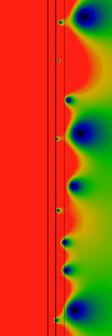
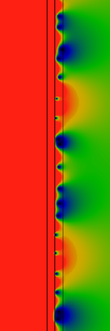
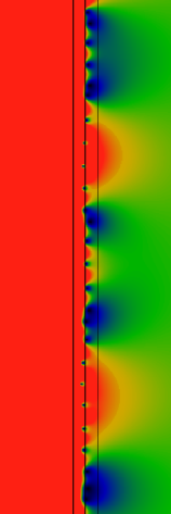
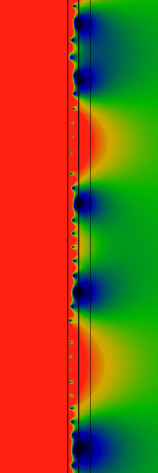
Figure 2: Riemann Sums

The above strip charts show $\left|\zeta_{N}(s)\right|$ for N=15, 151, 1051, 11051 and 151051 respectively. The three vertical black lines are located at $\Re s$=0, 1/2 and 1. The vertical range of these strips are all identical, ranging from $\Im s$=13 at the bottom, to $\Im s$=34 at the top. The coloration is such that red represents values greater than two, green for values about equal to one, and blue/black for values near/at zero. In this particular strip, we expect the exact Riemann zeta to have five zeros, near 14.13, 21.02, 25.01, 30.42, and 32.93. Several remarkable properties are visible: First, there are far more than five zeros visible, some lying outside the critical strip. Next, as the value of $N$ increases, the zeros migrate towards the $\Re s=1/2$ line; however, the number of zeros seems to multiply logarithmically as well. Most of these zeroes seem to have a tiny residue, which diminishes as $N$ increases; presumably, they will completely disappear in the limit. What’s left are five zeros which are not fading away; these become the Riemann zeroes.

 

The convergence properties of this sum, as well as the nature of the “artifact zeros”, can be understood by exploring the phase of $\zeta_{N}$ along the critical axis. This is shown in figure 3. Truncation at finite $N$ introduces a quasi-sinusoidal perturbation overlaid on the “true” Riemann zeta function.

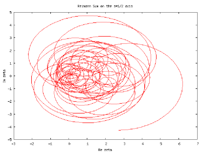
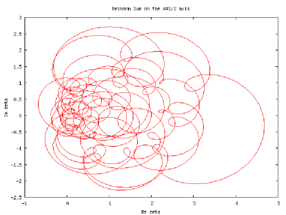
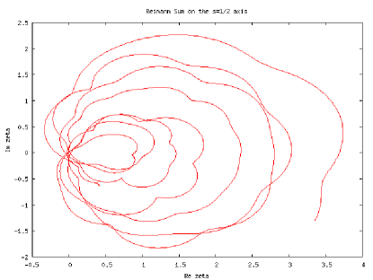
Figure 3: Riemann sum phase plots

The above three figures are parametric phase plots of $\zeta_{N}(s)$ for N=1051, 11051 and 121051, treating $s$ as a parameter, varying from $\Im s$=13 to 34 along the $\Re s=1/2$ line. That is, the graphs show $\Re\zeta_{N}$ on the x-axis, and $\Im\zeta_{N}$ along the y-axis as $s$ varies. The large number of zeros in the critical strip can be understood as being due to the looping seen in these graphs. As $N$ increases, the loops shrink, passing through cusps; the last figure beginning to resemble the true phase portrait of the Riemann zeta.

 

Armed with this overview, one may now explore the sum $\zeta_{N;1,2}$. As figure 4 shows, the simplest numerical evidence seems to directly support the hypothesis. The evidence for the hypothesis, in the case of $\zeta_{N;1,3}$ and $\zeta_{N;2,3}$ is less clear, as seen in figure 5. On the other hand, the numeric sums, for any fixed $N$, are far less “accurate” than that for $\zeta_{N;1,2}$. That is, the discontinuities for $S_{1,3}$ and $S_{2,3}$ are very finely spaced, and the summation does a considerably poorer job of capturing these.

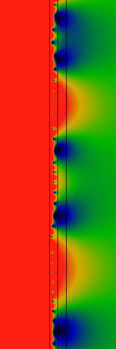
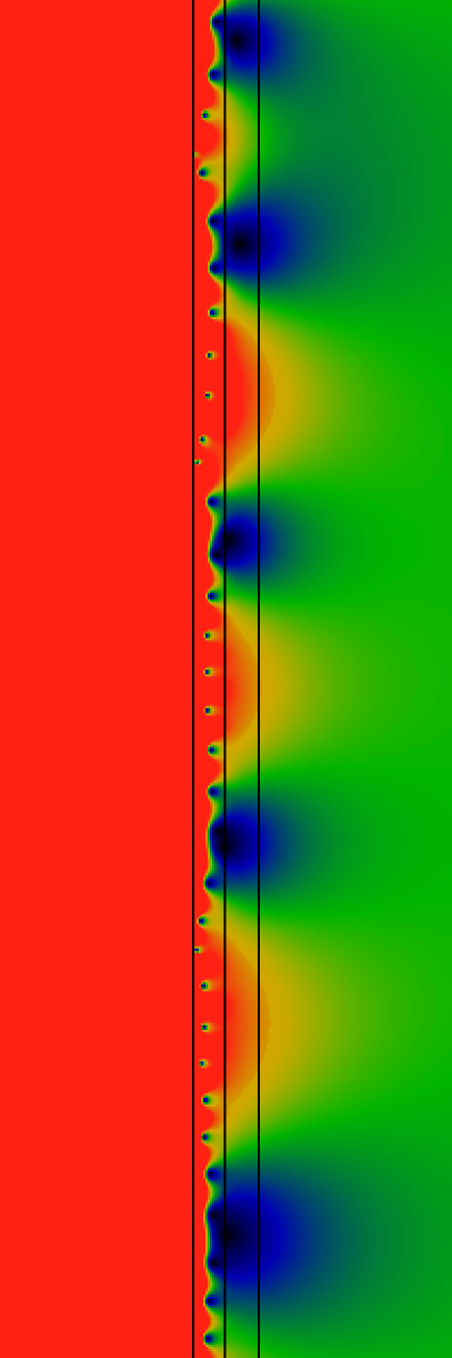
Figure 4: Zeros of $S_{1,2}$

This figure shows a side-by-side comparison of $\left|\zeta_{N}(s)\right|$ and $\left|\zeta_{N;1,2}(s)\right|$, with the later as defined in equation3, and $N=151051$. The sizes, heights and color scheme are as in the previous figures. Note the near-correspondence of the dominant zeros; yet, the zeros for $\left|\zeta_{N;1,2}(s)\right|$ do appear to be at shifted locations.

 

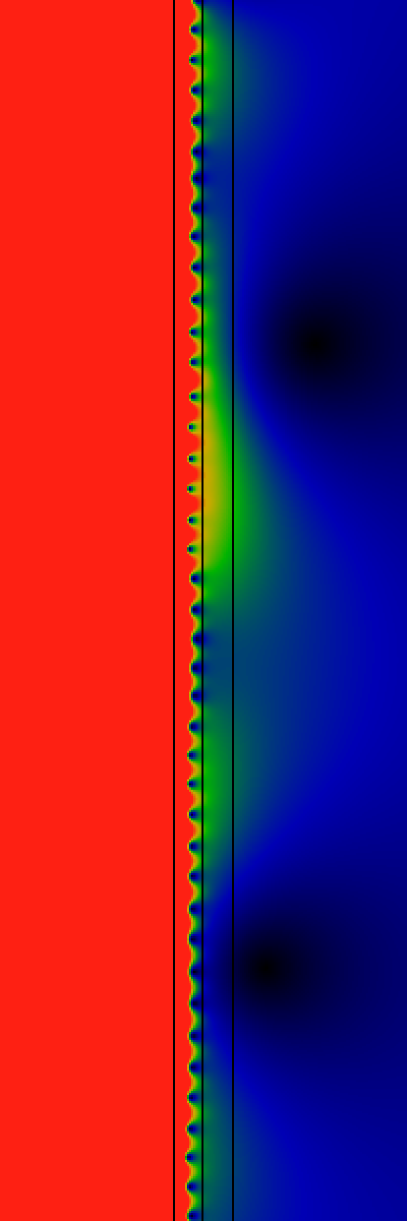
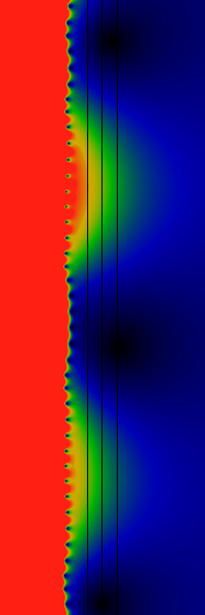
Figure 5: Zeros of $S_{1,3}$ and $S_{2,3}$

This figure shows a side-by-side comparison of $\left|\zeta_{N;1,3}(s)\right|$ and $\left|\zeta_{N;2,3}(s)\right|$, with the later as defined in equation3, and $N=151051$. The sizes, heights and color scheme are as in the previous figures. The dominant zeros no longer resemble those of $\left|\zeta_{N}(s)\right|$, and it is no longer clear whether they will end up in the critical strip. However, it is also the case that the structure of $S_{1,3}(x)$ and $S_{2,3}(x)$ is much finer and detailed, and so this value of $N$ does not yet provide an adequate visual estimate of the $N\to\infty$ form of these figures.

 

4 A Remarkable Shadow

The numerical evaluation of sums requires a certain amount of cross-checking so as to catch errors. A particularly curious sum to evaluate is

$$\eta_{N}(s)=\frac{s}{s-1}-\frac{s}{N}\;\sum_{n=0}^{N-1}\left(\frac{2n+1}{2N}\right)^{s}$$

which does no permutation at all. That is, one effectively has $\eta_{N}(s)=\zeta_{N;p,p}(s)$ for any integer $p$. The limiting integral is trivial to calculate, since $S_{p,p}(x)=x$, and so

$$\lim_{N\to\infty}\eta_{N}(s)=\frac{2s}{s^{2}-1}$$

Thus, this sum shouldn’t be interesting, except as a calibration of sorts.

But that is false. A review of the figure 6 shows that this simple stair-step sum retains traces of the locations of the non-trivial Riemann zeros!

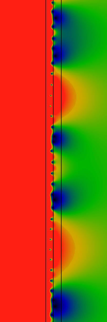
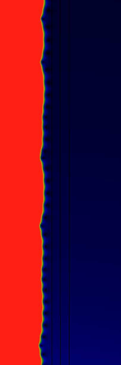
Figure 6: A Shadow of Zeta

This figure compares $\left|\zeta_{N}(s)\right|$ and $\left|\eta_{N}(s)\right|$ for $N=11051$. Note the “horns” or “cusps” in $\left|\eta_{N}(s)\right|$. While these are falling well outside the critical strip, it is particularly remarkable that they line up vertically with the locations of the non-trivial Riemann zeros.

 

The presence of this shadow is not hard to explain. Define

$$Z_{N}(s)=\sum_{n=1}^{N}\frac{1}{n^{s}}$$

Then it is clear that, for large $N$, $Z_{N}(s)$will approximate the Riemann zeta function:

$$\lim_{N\to\infty}Z_{N}(s)=\zeta(s)$$

at least for the case of $\Re s>1$, where the sum is convergent. With some simple manipulations, one may rewrite the numeric sum as

$$\sum_{n=0}^{N-1}\left(\frac{2n+1}{2N}\right)^{s}=\frac{1}{(2N)^{s}}\left[Z_{2N-1}(-s)-2^{s}Z_{N-1}(-s)\right]$$

The fact that the seemingly “trivial” $\eta_{N}(s)$ sum contains this approximation to the zeta would seem to explain the numeric features shown in figure 6. Furthermore, the presence of the $-s$ in the arguments appears to explain why the horns are located not far from the $\Re s=-1/2$ line.

On the other hand, there is another important lesson to be drawn here: this “trivial” sum is insufficient to explain the features seen in the $\zeta_{N;p,q}(s)$ sums. That is, although the numerical evaluation itself is prone to introducing the Riemann zeta as an artifact, the strength of this artifact does not immediately appear to be dominant enough to account for the entire behavior of the $\zeta_{N;p,q}(s)$ sums.

5 Sums and Integrals

This section explores analytic approaches to evaluating the integral 2. Because $S_{p,q}\left(x\right)$ is a piecewise combination of Mobius functions

$$\frac{ax+b}{cx+d}$$

it is enough to evaluate the indefinite integral

$$\int\frac{ax+b}{cx+d}x^{s-1}dx$$

This integral does not have any simple, closed-form solution, but can be given in terms of an infinite sum. This may be obtained via the Newton series

$$\left(1+x\right)^{s}=\sum_{k=0}^{\infty}\dbinom{s}{k}x^{k}$$

where

$$\binom{s}{k}=\frac{\Gamma\left(s+1\right)}{\Gamma\left(k+1\right)\Gamma\left(s-k+1\right)}$$

is the binomial coefficient. The series is absolutely convergent on the unit interval $0\leq x\leq 1$ that we wish to explore. The indefinite integral may then be evaluated as a sum:

$$F\left(s,\alpha;x\right)= \int\frac{x^{s}}{x+\alpha}dx$$

$$= \int\frac{\left(y-\alpha\right)^{s}}{y}dy$$

$$= \left(-\alpha\right)^{s}\sum_{k=0}^{\infty}\binom{s}{k}\left(\frac{-1}{\alpha}\right)^{k}\int y^{k-1}dy$$

$$= \left(-\alpha\right)^{s}\left[\ln\left(x+\alpha\right)+\sum_{k=1}^{\infty}\frac{\left(-1\right)^{k}}{k}\binom{s}{k}\left(1+\frac{x}{\alpha}\right)^{k}\right]$$

This allows the Mobius integral to be written as

$$\int\frac{ax+b}{cx+d}x^{s-1}dx=\frac{a}{c}F\left(s,\frac{d}{c};x\right)+\frac{b}{c}F\left(s-1,\frac{d}{c};x\right)$$

Using that fact that, in general, for continued fractions, the $a,b,c$ and $d$ will be integers, with $ad-bc=\pm 1$, one may re-write the above as

$$\int\frac{ax+b}{cx+d}x^{s-1}dx=\frac{\left(-d\right)^{s-1}}{c^{s+1}}\left[\mp\ln\left(x+\frac{d}{c}\right)+\sum_{k=1}^{\infty}\frac{\left(-1\right)^{k}}{k}\binom{s-1}{k}\left(1+\frac{cx}{d}\right)^{k}\left(\frac{\pm s+kbc}{k-s}\right)\right]$$ (4)

For $S_{1,2}\left(x\right)$, this can be made more explicit. So, we have that

$$S_{1,2}\left(x\right)=\frac{1}{a_{2}+\frac{1}{a_{1}+r}}$$

when $x$ is written as

$$x=\frac{1}{a_{1}+\frac{1}{a_{2}+r}}$$

with $a_{1}=\left\lfloor 1/x\right\rfloor$ and $a_{2}=\left\lfloor x/\left(1-a_{1}x\right)\right\rfloor$ integers. Solving for $r$ and replacing, one gets

$$S_{1,2}\left(x\right)=\frac{ax+b}{cx+d}$$

with

$$a= 1+a_{1}\left(a_{2}-a_{1}\right)$$

$$b= a_{1}-a_{2}$$

$$c= \left(a_{2}-a_{1}\right)\left(1+a_{1}a_{2}\right)$$

$$d= 1+a_{2}\left(a_{1}-a_{2}\right)$$

Note that in this case, $ad-bc=1$ for all possible values of $a_{1}$ and $a_{2}$. This form is valid over the interval

$$\left(\underline{x},\overline{x}\right)=\left(\frac{a_{2}}{1+a_{1}a_{2}},\frac{1+a_{2}}{1+a_{1}+a_{1}a_{2}}\right)$$

and so one may combine these elements to write

$$\int_{0}^{1}S_{1,2}\left(x\right)x^{s-1}dx=\sum_{a_{1}=1}^{\infty}\sum_{a_{2}=1}^{\infty}\int_{\underline{x}}^{\overline{x}}\frac{ax+b}{cx+d}x^{s-1}dx$$ (5)

At this point, the ability to perform any further simple manipulations stops. The summations are only conditionally convergent; one cannot interchange the sum over $k$ with the sums over $a_{1}$, $a_{2}$. If one were to do so, one would quickly discover that, for fixed $k$, the sums over $a_{1}$, $a_{2}$ are logarithmically divergent. While this is not immediately obvious just be gazing at the sums, it is easily confirmed by numerically evaluating them.

One more avenue suggests itself, but then fails: one might consider applying the binomial expansion to the powers $\left(1+\frac{x}{\alpha}\right)^{k}$ that appear in the sum for $F\left(s,\alpha;x\right)$, and then exchanging the order of summations there. But this is not possible; the sums fail outright. Thus, it appears that there are no further (obvious) analytic techniques that one can apply to reduce the expression 5. One is then left to contemplate the numeric evaluation of 5. Naively, one might expect that doing so would offer considerable advantages over the numeric sum 3, but this is not at all the case; convergence is even slower, and fails more profoundly.

Thus, the remainder of this text uses only the sum 3 for numeric exploration. The position of the first non-trivial zero of $\zeta_{1,2}\left(s\right)$ is examined in the next section.

6 Locating the first zero

This section explores the numeric evidence for the location of the first zero of $\zeta_{1,2}\left(s\right)$. One may quickly discover that it must be near $s=\frac{1}{2}+i\,14.92$, but improving upon this value is remarkably difficult, given only the tools 3 and 5.

The summations 3 are straightforward to evaluate numerically. Estimates for the location of the zero may be obtained using more-or-less standard zero-finding techniques, such as Powell’s algorithm[3] (some care must be taken, as the neighborhood of the zero appears to be a bit wobbly). The resulting estimates for the zero depend very strongly on $N$, and are very noisy, as the figure 7 shows. The noise appears to be classic fractal $1/f$ noise, as can be seen from the graph of the power spectrum.

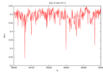
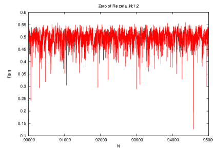
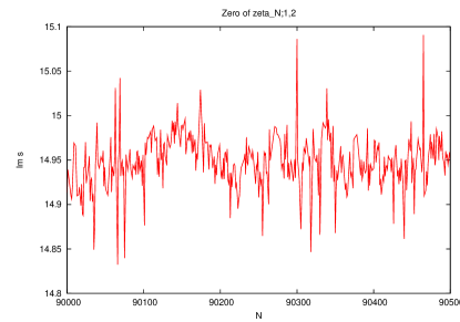
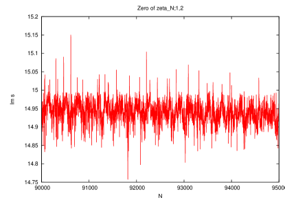
Figure 7: Numerical zero-finding

The above graphs show the location of the first non-trivial zero of $\zeta_{N;1,2}\left(s\right)$, as a function of $N$, in the range of $90000\leq N\leq 95000$. As may be seen, the location of the zero depends very strongly on $N$, and is an extremely noisy function of $N$. There is the vaguest hint of an oscillatory behavior in $N$, possibly with a period of $\Delta N=300$, but this is very strongly obscured by the noise. The power spectrum of this same data-set is examined in the next figure.

 

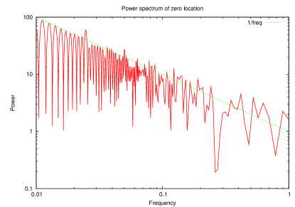
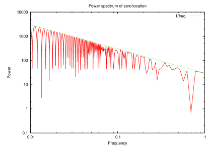
Figure 8: Power spectrum

These two charts show the power spectrum of the zero locations graphed in figure 7. The power spectrum is defined as usual, it is the square of the Fourier transform of the data. The straight line shows the $1/f$ spectrum; the noise in the location of the zero clearly obeys the classic fractal $1/f$ power density. The regular pattern of arches appearing at low frequencies is a numerical artifact resulting from the limited size of the data sample. The left chart shows the power along the real axis (resulting in the uncertainty of the $\Re s=\frac{1}{2}$ location), while the right chart shows the power in the imaginary direction. The higher power in the right chart indicates that the location $\Im s\approx 14.92$ is more certain than the location $\Re s\approx\frac{1}{2}$. Curiously, the “more important” location is harder to pin down!

 

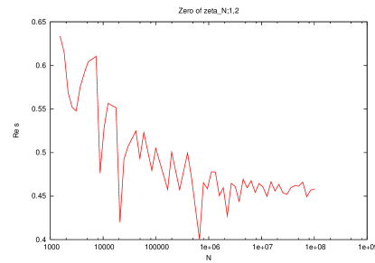
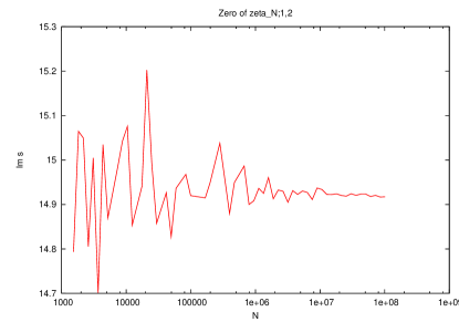
Figure 9: Increased precision

The above graphs show the location of the first non-trivial zero of $\zeta_{N;1,2}\left(s\right)$, as a function of $N$, on a logarithmic scale. Only a sparse set of values of $N$ are sampled. The figure on the left, which would confirm or disprove the conjecture, is ambiguous. Although the data, as illustrated, shows a precipitous drop past the critical line $\Re s=\frac{1}{2}$, it is not yet obvious whether there will be a bounce/oscillation back up towards $\Re s=\frac{1}{2}$, or whether the asymptotic behavior aims at $\Re s\simeq 0.45$. Unfortunately, computational costs are large; each additional point in these graphs requires in excess of a week of compute time on current-era computers.

 

7 Conclusions

Numerical evidence suggests that the permutation-inspired zeta

$$\zeta_{p,q}(s)=\lim_{N\to\infty}\zeta_{N;p,q}(s)$$

obeys a Riemann hypothesis, in that it’s zeros lie in the critical strip, and particularly on the $\Re s=1/2$ line. High-precision numerical computations are difficult, and offer only ambiguous support for the conjecture. Curiously, the numerical evaluation itself “accidentally” introduces some zeta-like artifacts, these artifacts do not seem to be sufficiently strong to explain the overall structure. Alternate approaches to the problem are desired, but the author is not aware of any particular theoretical framework that would be applicable, and could be employed to provide deeper insight into the phenomenon.

References

- [1] H.M. Edwards. Riemann’s Zeta Function. Dover Publications, 1972.
- [2] A. Ya. Khinchin. Continued Fractions. Dover Publications, (reproduction of 1964 english translation of the original 1935 russian edition) edition, 1997.
- [3] William H. Press, Saul A. Teukolsky, William T. Vetterling, and Brian P. Flannery. Numerical Recipes in C, The Art of Scientific Computing. Cambidge University Press, 2nd edition edition, 1988.
- [4] Linas Vepstas. On the minkowski measure. ArXiv, arXiv:0810.1265, 2008.