Measuring support for a hypothesis about a random parameter without estimating its unknown prior

Abstract

For frequentist settings in which parameter randomness represents variability rather than uncertainty, the ideal measure of the support for one hypothesis over another is the difference in the posterior and prior log odds. For situations in which the prior distribution cannot be accurately estimated, that ideal support may be replaced by another measure of support, which may be any predictor of the ideal support that, on a per-observation basis, is asymptotically unbiased. Two qualifying measures of support are defined. The first is minimax optimal with respect to the population and is equivalent to a particular Bayes factor. The second is worst-sample minimax optimal and is equivalent to the normalized maximum likelihood. It has been extended by likelihood weights for compatibility with more general models.

One such model is that of two independent normal samples, the standard setting for gene expression microarray data analysis. Applying that model to proteomics data indicates that support computed from data for a single protein can closely approximate the estimated difference in posterior and prior odds that would be available with the data for 20 proteins. This suggests the applicability of random-parameter models to other situations in which the parameter distribution cannot be reliably estimated.

Running headline: Support for a random hypothesis

David R. Bickel
Ottawa Institute of Systems Biology
Department of Biochemistry, Microbiology, and Immunology
University of Ottawa

Keywords: empirical Bayes; indirect evidence; information for discrimination; minimum description length; model selection; multiple comparisons; multiple testing; normalized maximum likelihood; strength of statistical evidence; weighted likelihood

1 Introduction

The p-value has now served science for a century as a measure of the incompatibility between a simple (point) null hypothesis and an observed sample of data. The celebrated advantage of the p-value is its objectivity relative to Bayesian methods in the sense that it is based on a model of frequencies of events in the world rather than on a model that describes the beliefs or decisions of an ideal agent.

On the other hand, the Bayes factor has the salient advantage that it is easily interpreted in terms of combining with previous information. Unlike the p-value, it is a measure of support for one hypothesis over another; that is, it quantifies the degree to which the data change the odds that the hypothesis is true, whether or not a prior odds is available in the form of known frequencies. Although the Bayes factor does not depend on a prior probability of hypothesis truth, it does depend on which priors are assigned to the parameter distribution under the alternative hypothesis unless that alternative hypothesis is simple, in which case the Bayes factor reduces to the likelihood ratio if the null hypothesis is also simple. Unfortunately, the improper prior distributions generated by conventional algorithms cannot be directly applied to the Bayes factor. That has been overcome to some extent by dividing the data into training and test samples, with the training samples generating proper priors for use with test samples, but at the expense of requiring the specification of training samples and, when using multiple training samples, a method of averaging (Berger and Pericchi, 1996).

On the basis of concepts defined in Section 2, Section 3 will marshal results of information theory to seize the above advantages of the p-value and Bayes factor by deriving measures of hypothesis support of wide applicability that are objective enough for routine scientific reporting. While such results have historically been cast in terms of minimum description length (MDL), an idealized minimax length of a message encoding the data, they will be presented herein without reliance on that analogy. For the present paper, it is sufficient to observe that the proposed level of support for one hypothesis over another is the difference in their MDLs and that Rissanen (1987) used a difference in previous MDLs to compare hypotheses.

To define support in terms of the difference between posterior and prior log-odds without relying on non-frequency probability, Section 2.2 will relate the prior probability of hypothesis truth to the fraction of null hypotheses that are true. This framework is the two-groups model for the analysis of gene expression data by empirical Bayes methods (Efron et al., 2001) and later adapted to other data of high-dimensional biology such as those of genome-wide association studies (Efron, 2010b; Yang and Bickel, 2010, and references) and to data of medium-dimensional biology such as those of proteins and metabolites (Bickel, 2010a, b). In such applications, each gene or other biological feature corresponds to a different random parameter, the value of which determines whether its null hypothesis is true.

While the proposed measures of hypothesis support fall under the two-groups umbrella, they are not empirical Bayes methods since they operate without any estimation or knowledge of prior distributions. Nonetheless, the unknown prior is retained in the model as a distribution across random parameters, including but not necessarily limited to those that generate the observed data.

Thus, the methodology of this paper is applicable to situations in which reliable estimation the unknown two-groups prior is not possible. Such situations often arise in practice. For example, the number of random parameters for which measurements are available and that have sufficient independence between parameters is often considered too small for reliable estimation of the prior distribution. Qiu et al. (2005) argued that, due to correlations in expression levels between genes, this is the case with microarray data. Less controversially, few would maintain that the prior can be reliably estimated when only one random parameter generated data, e.g., when the expression of only a single gene has been recorded. Another example is the setting in which the data cannot be reduced to continuous test statistics that adequately meet the assumptions of available empirical Bayes methods of estimating the prior distribution.

Section 2 fixes basic notation and explains the two-groups model. Under that framework, Section 3 defines support for one hypothesis over another in terms of a difference between the posterior and prior log-odds. Thus, reporting support in a scientific paper enables each reader to roughly determine what the posterior probability of either hypothesis would be using a different hypothetical value of its unknown prior probability. Section 4 then gives two qualifying measures of support, each of which is minimax optimal in a different sense. In Section 5, one of the optimal measures is compared to empirical Bayes methodology using real proteomics data. That case study addresses the extent to which optimal support on the basis of abundance measurements of a single protein can approximate the analogous value that would be available in the presence of measurements across multiple proteins. Finally, Section 6 closes with a concluding summary.

2 Preliminaries

2.1 Distributions given the parameter values

For all $i\in\left\{1,\dots,N\right\}$, the observed data vector $x_{i}$ of $n$ observations is assumed to be the outcome of $X_{i}$, the random variable of density function $f\left(\bullet|\phi_{i}\right)$ on sample space $\mathcal{X}^{n}$ for some $\phi_{i}$ in parameter space $\Phi$. Hypotheses about $\phi_{i}$, called the full parameter, are stated in terms of the subparameter $\theta_{i}=\theta\left(\phi_{i}\right)$, called the parameter of interest, which lies in a set $\Theta$. Consider the member $\theta_{0}$ of $\Theta$ in order to define the null hypotheses $\theta_{1}=\theta_{0}$, $\dots$, $\theta_{i}=\theta_{0}$, $\dots$, $\theta_{N}=\theta_{0}$. The conditional density notation reflects the randomness of the parameter to be specified in Section 2.2.

A measurable map $\tau:\mathcal{X}^{n}\rightarrow\mathcal{T}$ yields $t_{i}=\tau\left(x_{i}\right)$ as the observed value of the random test statistic $T_{i}=\tau\left(X_{i}\right)$. The application of the map can often reduce the data to a lower-dimensions statistic, but the identity map may be employed if no reduction is desired: $T_{i}=X_{i}=\tau\left(X_{i}\right)$. In some cases, the map may be chosen to eliminate the nuisance parameter, which means the probability density function of $T_{i}$, conditional on $\theta_{i}$, may be written as $g\left(\bullet|\theta_{i}\right)$. Otherwise, the interest parameter is identified with the full parameter $\left(\theta_{i}=\theta\left(\phi_{i}\right)=\phi_{i}\right)$, in which case $g\left(\bullet|\theta_{i}\right)=f\left(\bullet|\phi_{i}\right)$. Thus, the following methodology applies even when the nuisance parameter cannot be eliminated by data reduction.

2.2 Hierarchical model

Let $P_{1}$ denote the alternative-hypothesis prior distribution, assumed to have measure-theoretic support $\Theta$, and let $\pi_{0}$ denote the probability that a given null hypothesis is true. (Unless prefaced by measure-theoretic, the term support in this paper means strength of statistical evidence (§1) rather than what it means in measure theory.) Like most hierarchical models, including those of empirical-Bayes and random-effects methods, this two-groups model uses random parameters to represent real variability rather than subjective uncertainty:

$$T_{i}\sim\pi_{0}g_{0}+\pi_{1}g_{1},$$ (1)

where $\pi_{1}=1-\pi_{0}$, and where $g_{0}=g\left(\bullet|\theta_{0}\right)$ and $g_{1}=\int g\left(\bullet|\theta\right)dP_{1}\left(\theta\right)$ are the null and alternative density functions, respectively.

Let $P$ denote a joint probability distribution of $\theta$ and $T_{i}$ such that $P_{1}=P\left(\bullet|\theta\neq\theta_{0}\right)$, $P\left(\theta=\theta_{0}\right)=\pi_{0}$, and $P\left(\bullet|\theta=\theta_{i}\right)$ admits $g\left(\bullet|\theta_{i}\right)$ as the density function of $T_{i}$ conditional on $\theta=\theta_{i}$ for all $\theta_{i}\in\Theta$. Let $A_{i}$ denote the random variable indicating whether, for all $i=1,\dots,N$, the $i$th null hypothesis is true $\left(A_{i}=0\right)$ or whether the alternative hypothesis is true $\left(A_{i}=1\right)$. For sufficiently large $N$ and sufficient independence between random parameters, $\pi_{0}$ approximates, with high probability, the proportion of the $N$ null hypotheses that are true.

Bayes’s theorem then gives

$$\frac{P\left(A_{i}=1|T_{i}=t_{i}\right)}{P\left(A_{i}=0|T_{i}=t_{i}\right)}=\frac{P\left(A_{i}=1\right)}{P\left(A_{i}=0\right)}\frac{g_{1}\left(t_{i}\right)}{g_{0}\left(t_{i}\right)}=\frac{\pi_{1}}{\pi_{0}}\frac{g_{1}\left(t_{i}\right)}{g_{0}\left(t_{i}\right)},$$ (2)

but that cannot be used directly without knowledge of $\pi_{0}$ and of $g_{1}$, which is unknown since $P_{1}$ is unknown. Since the empirical Bayes strategy of estimating those priors is not always feasible (§1), the next section presents an alternative approach for inference about whether a particular null hypothesis is true.

3 General definition of support

One distribution will be said to surrogate the other if it can represent or take the place of the other for inferential purposes. Before precisely defining surrogation, the reason for introducing the concept will be explained. Given $g_{1}^{\star}$, a probability density function that surrogates $g_{1}$, let $P^{\star}$ denote the probability distribution that satisfies both $P^{\star}\left(A_{i}=a\right)=P\left(A_{i}=a\right)$ for $a\in\left\{0,1\right\}$ and

$$\frac{P^{\star}\left(A_{i}=1|T_{i}^{\star}=t_{i}\right)}{P^{\star}\left(A_{i}=0|T_{i}^{\star}=t_{i}\right)}=\frac{P^{\star}\left(A_{i}=1\right)}{P^{\star}\left(A_{i}=0\right)}\frac{g_{1}^{\star}\left(t_{i}\right)}{g_{0}\left(t_{i}\right)},$$ (3)

where $T_{i}^{\star}$ has the mixture probability density function $\pi_{1}g_{1}^{\star}+\pi_{0}g_{0}$ rather than that of equation (1). Equation (2) and $P^{\star}\left(A_{i}=1\right)=P\left(A_{i}=1\right)$ entail that $P^{\star}\left(A_{i}=1|T_{i}^{\star}=t_{i}\right)$ surrogates $P\left(A_{i}=1|T_{i}=t_{i}\right)$ inasmuch as $g_{1}^{\star}$ surrogates $g_{1}$, which is unknown since it depends on $P_{1}$. Thus, posterior probabilities of hypothesis truth can be surrogated by using $g_{1}^{\star}$ in place of $g_{1}$. Although the surrogate posterior probability depends on the proportion $P^{\star}\left(A_{i}=1\right)=\pi_{1}$, the measure of support to be derived from equation (3) does not require that $\pi_{1}$ be known or even that it be estimated.

The concept of surrogation will be patterned after that of universality. Let $E_{\theta_{i}}$ stand for the expectation operator defined by $E_{\theta_{i}}\left(\bullet\right)=\int\bullet dP\left(\bullet|\theta=\theta_{i}\right)=\int\bullet g\left(t|\theta_{i}\right)dt$. A probability density function $g_{1}^{\star}$ is universal for the family $\left\{g\left(\bullet|\theta_{i}\right):\theta_{i}\in\Theta\right\}$ if, for any $\theta_{i}\in\Theta$, the Kullback-Leibler divergence $D\left(g\left(\bullet|\theta_{i}\right)\|g_{1}^{\star}\right)=E_{\theta_{i}}\left(\log\left[g\left(T_{i}|\theta_{i}\right)/g_{1}^{\star}\left(T_{i}\right)\right]\right)$ satisfies

$$\lim_{n\rightarrow\infty}D\left(g\left(\bullet|\theta_{i}\right)\|g_{1}^{\star}\right)/n=0.$$ (4)

The terminology comes from the theory of universal source coding (Grünwald, 2007, p. 200); $g_{1}^{\star}$ is called “universal” because it is a single density function typifying all of the distributions of the parametric family. Equation (4) may be interpreted as the requirement that the per-observation bias in $\log g_{1}^{\star}\left(T_{i}\right)$ as a predictor of $\log g\left(T_{i}|\theta_{i}\right)$ asymptotically vanishes. This lemma illustrates the concept of universality with an important example:

Lemma 1.

Let $\Pi$ denote a probability distribution that has measure-theoretic support $\Theta$. The mixture density $\bar{g}$ defined by $\bar{g}\left(t\right)=\int g\left(t|\theta\right)d\Pi\left(\theta\right)$ for all $t\in\mathcal{T}$ is universal for $\left\{g\left(\bullet|\theta_{i}\right):\theta_{i}\in\Theta\right\}$.

Proof.

By the stated assumption about $\Pi$, there is a $\tilde{\Theta}\subset\Theta$ such that $\theta_{i}\in\tilde{\Theta}$ and

$$\int g\left(t|\theta\right)d\Pi\left(\theta\right)\geq\sup_{\tilde{\theta}\in\tilde{\Theta}}g\left(t|\tilde{\theta}\right)\int_{\tilde{\Theta}}d\Pi\left(\theta\right)$$ (5)

for all $\theta_{i}\in\Theta$ and $t\in\mathcal{T}$. With $\sup_{\tilde{\theta}\in\tilde{\Theta}}g\left(t|\tilde{\theta}\right)\geq g\left(t|\theta_{i}\right)$ and $\bar{g}\left(t\right)=\int g\left(t|\theta\right)d\Pi\left(\theta\right)$, inequality (5) entails that

$$\lim_{n\rightarrow\infty}\frac{\log\bar{g}\left(t\right)}{n}\geq\lim_{n\rightarrow\infty}\frac{\log g\left(t|\theta_{i}\right)+\log\int_{\tilde{\Theta}}d\Pi\left(\theta\right)}{n}=\lim_{n\rightarrow\infty}\frac{\log g\left(t|\theta_{i}\right)}{n}$$

for all $\theta_{i}\in\Theta$ and $t\in\mathcal{T}$. While that yields $\lim_{n\rightarrow\infty}D\left(g\left(\bullet|\theta_{i}\right)\|\bar{g}\right)/n\leq 0$, the information inequality has $D\left(g\left(\bullet|\theta_{i}\right)\|\bar{g}\right)\geq 0$. The universality of $\bar{g}$ then follows from equation (4). (This proof generalizes a simpler argument using probability mass functions (Grünwald, 2007, p. 176).) ∎

Universality suggests a technical definition for surrogation. With respect to the family $\left\{g\left(\bullet|\theta_{i}\right):\theta_{i}\in\Theta\right\}$, a probability density function $g^{\prime}$ surrogates any probability density function $g^{\prime\prime}$ for which

$$\lim_{n\rightarrow\infty}E_{\theta_{i}}\left(\log\left[g^{\prime}\left(T_{i}\right)/g^{\prime\prime}\left(T_{i}\right)\right]\right)/n=0$$ (6)

for all $\theta_{i}\in\Theta$. The idea is that one distribution can represent or take the place of another for inferential purposes if their mean per-observation difference vanishes asymptotically. The following lemma then says that any universal distribution can stand in the place of any other distribution that is universal for the same family. It is a direct consequence of equations (4) and (6).

Lemma 2.

If the probability density functions $g^{\prime}$ and $g^{\prime\prime}$ are universal for $\left\{g\left(\bullet|\theta_{i}\right):\theta_{i}\in\Theta\right\}$, then $g^{\prime}$ surrogates $g^{\prime\prime}$ with respect to $\left\{g\left(\bullet|\theta_{i}\right):\theta_{i}\in\Theta\right\}$.

The inferential use of one density function in place of another calls for a concept of surrogation error. The surrogation error of each probability distribution $P^{\star}$ based on the probability density function $g_{1}^{\star}$ in place of $g_{1}$ is defined by

$$\varepsilon^{\star}\left(t\right)=\log\frac{P^{\star}\left(A_{i}=1|T_{i}^{\star}=t\right)}{P^{\star}\left(A_{i}=0|T_{i}^{\star}=t\right)}-\log\frac{P\left(A_{i}=1|T_{i}=t\right)}{P\left(A_{i}=0|T_{i}=t\right)}.$$

Then $P^{\star}$ is said to surrogate $P$ if

$$\lim_{n\rightarrow\infty}E_{\theta_{i}}\varepsilon^{\star}\left(T_{i}\right)/n=0$$ (7)

for all $i=1,\dots,N$ and $a\in\left\{0,1\right\}$. Equation (7) states the criterion that the per-observation bias in $\log\left[P^{\star}\left(A_{i}=1|T_{i}^{\star}=T_{i}\right)/P^{\star}\left(A_{i}=0|T_{i}^{\star}=T_{i}\right)\right]$ as a predictor of the true posterior log odds asymptotically vanishes. This bias is conservative:

Proposition 3.

If $P^{\star}$ is based on a density function $g_{1}^{\star}$ on $\mathcal{T}$, then $E_{\theta_{i}}\varepsilon^{\star}\left(T_{i}\right)\leq 0$ for all $\theta_{i}\in\Theta$.

Proof.

The following holds for all $i=1,\dots,N$. By equations (2) and (3) with $P^{\star}\left(A_{i}=a\right)=P\left(A_{i}=a\right)$ for $a\in\left\{0,1\right\}$,

$$E_{\theta_{i}}\varepsilon^{\star}\left(T_{i}\right)=-D\left(g_{1}\|g_{1}^{\star}\right),$$

but $D\left(g_{1}\|g_{1}^{\star}\right)\geq 0$ by the information inequality. ∎

The next result connects the concepts of surrogation (asymptotic per-observation unbiasedness) and universality.

Theorem 4.

If $P^{\star}$ is based on a density function $g_{1}^{\star}$ that is universal for $\left\{g\left(\bullet|\theta_{i}\right):\theta_{i}\in\Theta\right\}$, then it surrogates $P$.

Proof.

Since $P_{1}$ has measure-theoretic support $\Theta$, Lemma 1 implies that $g_{1}$ is universal for $\left\{g\left(\bullet|\theta_{i}\right):\theta_{i}\in\Theta\right\}$. The universality of $g_{1}$ and $g_{1}^{\star}$ for $\left\{g\left(\bullet|\theta_{i}\right):\theta_{i}\in\Theta\right\}$ then entails that $g_{1}^{\star}$ surrogates $g_{1}$ by Lemma 2. According to equation (6), such surrogation means

$$\lim_{n\rightarrow\infty}E_{\theta_{i}}\left(\log\left[g_{1}^{\star}\left(T_{i}\right)/g_{1}\left(T_{i}\right)\right]\right)/n=0.$$ (8)

By equations (2) and (3) with $P^{\star}\left(A_{i}=a\right)=P\left(A_{i}=a\right)$ for $a\in\left\{0,1\right\}$,

$$\lim_{n\rightarrow\infty}E_{\theta_{i}}\varepsilon^{\star}\left(T_{i}\right)/n=\lim_{n\rightarrow\infty}E_{\theta_{i}}\left(\log\left[g_{1}^{\star}\left(T_{i}\right)/g_{1}\left(T_{i}\right)\right]\right)/n,$$

which equation (8) says is equal to 0. ∎

The difference in conditional and marginal log-odds,

$$S^{\star}\left(t_{i}\right)=\log\frac{P^{\star}\left(A_{i}=1|T^{\star}=t_{i}\right)}{P^{\star}\left(A_{i}=0|T^{\star}=t_{i}\right)}-\log\frac{P^{\star}\left(A_{i}=1\right)}{P^{\star}\left(A_{i}=0\right)},$$ (9)

is called the support that the observation $t_{i}$ transmits to the hypothesis that $\theta_{i}\neq\theta_{0}$ over the hypothesis that $\theta_{i}=\theta_{0}$ according to $P^{\star}$, which by assumption surrogates $P$. While the concise terminology follows Edwards (1992), the basis on a change in log-odds is that of the information for discrimination (Kullback, 1968). Royall (2000a), Blume (2002), and others have used the term strength of statistical evidence as a synonym for support in the original sense of Edwards (1992).

Proposition 5.

If $P^{\star}$ surrogates $P$ based on the universal density function $g_{1}^{\star}$, then the support that the observation $t_{i}$ transmits to the hypothesis that $\theta_{i}\neq\theta_{0}$ over the hypothesis that $\theta_{i}=\theta_{0}$ according to $P^{\star}$ is

$$S^{\star}\left(t_{i}\right)=\log\frac{g_{1}^{\star}\left(t_{i}\right)}{g_{0}\left(t_{i}\right)}.$$ (10)

Proof.

Substituting the solution of equation (9) for $g_{1}^{\star}\left(t_{i}\right)/g_{0}\left(t_{i}\right)$ into equation (10) recovers equation (9). ∎

Since the support according to $P^{\star}$ only depends on $P^{\star}$ through its universal density, $S\left(t_{i};g_{1}^{\star}\right)=\log\left(g_{1}^{\star}\left(t_{i}\right)/g_{0}\left(t_{i}\right)\right)$ is more simply called the support that the observation $t_{i}$ transmits to the hypothesis that $\theta_{i}\neq\theta_{0}$ over the hypothesis that $\theta_{i}=\theta_{0}$ according to $g_{1}^{\star}.$ Hence, the same value of the support applies to different hypothetical values of $\pi_{0}$ and even across different density functions as $g_{1}$, the unknown alternative distribution of the reduced data.

4 Optimal measures of support

Equations (2) and (3) with $P^{\star}\left(A_{i}=a\right)=P\left(A_{i}=a\right)$ for $a\in\left\{0,1\right\}$ imply that the surrogation error of $P^{\star}$ is equal to the surrogation error of $g_{1}^{\star}\left(t\right)$,

$$\varepsilon^{\star}\left(t\right)=\log g_{1}^{\star}\left(t\right)-\log g_{1}\left(t\right),$$

which depends neither on $\pi_{0}$ nor on any other aspect of $P^{\star}$ apart from $g_{1}^{\star}$. Thus, the problem of minimizing the surrogation error of $P^{\star}$ reduces to that of optimizing the universal density $g_{1}^{\star}$ on which $P^{\star}$ is based. Such optimality may be either with respect to the population represented by $g_{1}$ or with respect to the observed sample reduced to $t_{i}$. The remainder of this section formalizes each type of optimality as a minimax problem with a worst-case member of $\left\{g\left(\bullet|\theta_{i}\right):\theta_{i}\in\Theta\right\}$ in place of the unknown mixture density $g_{1}=\int g\left(\bullet|\theta\right)dP_{1}\left(\theta\right)$.

4.1 Population optimality

Among all probability density functions on $\mathcal{T}$, let $g_{1}^{\star}$ be that which minimizes the maximum average log loss

$$\sup_{\theta_{i}\in\Theta}E_{\theta_{i}}\left(\log\frac{g\left(T_{i}|\theta_{i}\right)}{g_{1}^{\star}\left(T_{i}\right)}\right).$$ (11)

Since the loss at each $\theta_{i}$ is averaged over the population represented by the sampling density $g_{1}$, the solution $g_{1}^{\star}$ will be called the population-optimal density function relative to $\left\{g\left(\bullet|\theta_{i}\right):\theta_{i}\in\Theta\right\}$. That density function has the mixture density

$$g_{1}^{\star}\left(t\right)=\int g\left(t|\theta_{i}\right)p_{1}^{\star}\left(\theta_{i}\right)d\theta_{i}$$

for all $t\in\mathcal{T}$, where $p_{1}^{\star}$ is the probability density function on $\Theta$ that maximizes

$$\int D\left(g_{1}\|g_{1}^{\star}\right)p_{1}^{\star}\left(\theta_{i}\right)d\theta_{i}$$

(Rissanen, 2007, §5.2.1).

The prior density function $p_{1}^{\star}$ thereby defined is difficult to compute at finite samples but asymptotically approaches the Jeffreys prior (Rissanen, 2009, §2.3.2), which was originally derived for Bayesian inference from an invariance argument (Jeffreys, 1948). Whereas $P_{1}$ is an unknown distribution of parameter values that describe physical reality, $p_{1}^{\star}$ is a default prior that serves as a tool for inference for scenarios in which suitable estimates of $P_{1}$ are not available. Lemma 1 secures the universality of $g_{1}^{\star}$, which in turn implies that $\log\left[g_{1}^{\star}\left(t_{i}\right)/g_{0}\left(t_{i}\right)\right]$ qualifies as support by Proposition 5.

For the observation $t_{i}$, $g_{1}^{\star}\left(t_{i}\right)$ may likewise be considered as a default integrated likelihood and the support (10) as the logarithm of a default Bayes factor. Drmota and Szpankowski (2004) reviewed asymptotic properties of the population-optimal density function and related it to the universal density function satisfying the optimality criterion of the next subsection.

4.2 Sample optimality

Among all probability density functions on $\mathcal{T}$, let $g_{1}^{\star}$ be the one that minimizes the maximum worst-case log loss

$$\sup_{\theta_{i}\in\Theta,t\in\mathcal{T}}\log\frac{g\left(t|\theta_{i}\right)}{g_{1}^{\star}\left(t\right)}.$$ (12)

Since the regret $\sup_{\theta_{i}\in\Theta}\log\left[g\left(t_{i}|\theta_{i}\right)/g_{1}^{\star}\left(t_{i}\right)\right]$ incurred by any observed sample $t_{i}$ is no greater than that of the worst-case sample, $g_{1}^{\star}$ will be referred to as the sample-optimal density function relative to $\left\{g\left(\bullet|\theta_{i}\right):\theta_{i}\in\Theta\right\}$. As proved by Shtarkov (1987), the unique solution to that minimax problem is

$$g_{1}^{\star}=\frac{g\left(\bullet;\hat{\theta}_{i}\left(\bullet\right)\right)}{\int_{\mathcal{T}}g\left(t;\hat{\theta}_{i}\left(t\right)\right)dt},$$ (13)

with the normalizing constant $Z=\int_{\mathcal{T}}g\left(t;\hat{\theta}_{i}\left(t\right)\right)dt$ automatically acting as a penalty for model complexity, where the maximum likelihood estimate (MLE) for any $t\in\mathcal{T}$ is denoted by $\hat{\theta}_{i}\left(t\right)=\arg\sup_{\theta_{i}\in\Theta}g\left(t|\theta_{i}\right)$ (Rissanen, 2007; Grünwald, 2007). The probability density $g_{1}^{\star}\left(t_{i}\right)$ is thus known as the normalized maximum likelihood (NML). Its universality (4) follows from the convergence of

$$\frac{D\left(g_{1}\|g_{1}^{\star}\right)}{n} = \frac{E_{\theta_{i}}\left(\log\left[g\left(T_{i}|\theta_{i}\right)/g\left(T_{i};\hat{\theta}_{i}\left(T_{i}\right)\right)\right]\right)}{n}+\frac{\log Z}{n}$$

to 0, which holds under the consistency of $\hat{\theta}_{i}\left(T_{i}\right)$ since the growth of $\log Z$ is asymptotically proportional to $\log n$ (Rissanen, 2007; Grünwald, 2007). Thus, Proposition 5 guarantees that $\log\left[g_{1}^{\star}\left(t_{i}\right)/g_{0}\left(t_{i}\right)\right]$ measures support.

For inference about $\theta_{i}$, the incidental statistics $t_{1},\dots,t_{i-1},t_{i+1},\dots,t_{N}$ provide side information or “indirect evidence” (Efron, 2010a) in addition to the “direct evidence” provided by the focus statistic $t_{i}$. The problem of incorporating side information into inference has been addressed with the weighted likelihood function $\bar{L}_{i}\left(\bullet;t_{i}\right)$ (Hu and Zidek, 2002; Wang and Zidek, 2005) defined by

$$\log\bar{L}_{i}\left(\theta_{i};t_{i}\right)=\sum_{j=1}^{N}w_{ij}\log g\left(t_{j}|\theta_{i}\right),$$ (14)

for all $\theta_{i}\in\Theta$, where the focus weight $w_{ii}$ is no less than any of the incidental weights $w_{ij}$ $\left(j\neq i\right)$. For notational economy and parallelism with $g\left(t_{i}|\theta_{i}\right)$, the left-hand side expresses dependence on the focus statistic but not on the incidental statistics.

Replacing the likelihood function in equation (12) with the weighted likelihood function, while taking the worst-case sample of the focus statistic and holding the incidental statistics fixed, has the unique solution

$$g_{1i}^{\star}=\frac{\bar{L}_{i}\left(\bar{\theta}_{i}\left(\bullet\right);\bullet\right)}{\int_{\mathcal{T}}\bar{L}_{i}\left(\bar{\theta}_{i}\left(t\right);t\right)dt},$$ (15)

where the maximum weighted likelihood estimate (MWLE) for any $t\in\mathcal{T}$ is denoted by $\bar{\theta}_{i}\left(t\right)=\arg\sup_{\theta\in\Theta}\bar{L}_{i}\left(\theta;t\right)$ (Bickel, 2010b). Accordingly, $g_{1i}^{\star}$ will be called the sample-optimal density function relative to $\left\{g\left(\bullet|\theta_{i}\right):\theta_{i}\in\Theta\right\}$ and $w_{i1},\dots,w_{iN}$. If $w_{ij}=\left(n+1\right)^{-1}\left(N-1\right)^{-1}$ for all $j\neq i$ and $w_{ii}=1-\left(n+1\right)^{-1}$, then $w_{i1},\dots,w_{iN}$ are single-observation weights in the sense that $\sum_{j\neq i}w_{ij}=w_{ii}/n$ (Bickel, 2010b). In accordance with equation (10), the corresponding sample-optimal support is $S_{i}^{\star}\left(t_{i}\right)=\log\left[g_{1i}^{\star}\left(t_{i}\right)/g_{0}\left(t_{i}\right)\right]$. When data are only available for one of the $N$ populations, the NMWL using single-observation weights may be closely approximated by considering

$$\log\bar{L}_{1}\left(\theta_{1};t_{1}\right)=\left(n+1\right)^{-1}\log g\left(t_{0}|\theta_{1}\right)+\left(1-\left(n+1\right)^{-1}\right)\log g\left(t_{1}|\theta_{1}\right)$$ (16)

as the logarithm of the weighted likelihood, where $t_{0}$ is a pseudo-observation such as the mode of $T_{1}$ under the null hypothesis (Bickel, 2010b).

The probability density $g_{1i}^{\star}\left(t_{i}\right)$ is called the normalized maximum weighted likelihood (NMWL). It applies to more general contexts than the NML: there are many commonly used distribution families for which $\int_{\mathcal{T}}\bar{L}_{i}\left(\bar{\theta}_{i}\left(t\right);t\right)dt$ but not $\int_{\mathcal{T}}g\left(t;\hat{\theta}_{i}\left(t\right)\right)dt$ is finite (Bickel, 2010b). As with other extensions of the NML to such families (Grünwald, 2007, Chapter 11), conditions under which the NMWL is universal have yet to be established. Thus, Proposition 5 cannot be invoked at this time, and one may only conjecture that $S_{i}^{\star}\left(t_{i}\right)$ satisfies the general criterion of a measure of support (§3) in a particular context. The conjecture is suggested for the normal family by the finding of the next section that $g_{1i}^{\star}\left(t_{i}\right)$ can closely approximate a universal density even for very small samples.

5 Proximity to simultaneous inference: a case study

This section describes a case study on the extent to which support computed on the basis of measurements of the abundance of a single protein can approximate the true difference between posterior and prior log odds. Since that true difference is unknown, it will be estimated using an empirical Bayes method to simultaneously incorporate the available abundance measurements for all proteins.

Specifically, the individual sample-optimal support of each protein was compared to an estimated Bayes factor using levels of protein abundance in plasma as measured in the laboratory of Alex Miron at the Dana-Farber Cancer Institute. The participating women include 55 with HER2-positive breast cancer, 35 mostly with ER/PR-positive breast cancer, and 64 without breast cancer. The abundance levels, available in Li (2009), were transformed by shifting them to ensure positivity and by taking the logarithms of the shifted abundance levels (Bickel, 2010a).

The transformed abundance levels of protein $i$ were assumed to be IID normal within each health condition and with an unknown variance $\sigma_{i}^{2}$ common to all three conditions. For one of the cancer conditions and for the non-cancer condition, $\mu_{i}^{\text{cancer}}$ and $\mu_{i}^{\text{healthy}}$ will denote the means of the respective normal distributions, and $n^{\text{cancer}}\in\left\{55,35\right\}$ and $n^{\text{healthy}}=64$ will likewise denote the numbers of women with each condition. Let $T_{i}$ represent the absolute value of the Student $t$ statistic appropriate for testing the null hypothesis of $\theta_{i}=0$, where $\theta_{i}=\left|\delta_{i}\right|$ and

$$\delta_{i}=\frac{\mu_{i}^{\text{cancer}}-\mu_{i}^{\text{healthy}}}{\sigma_{i}/\left(m^{-1}+n^{-1}\right)^{-1/2}},$$

the standardized cancer-healthy difference in the population mean transformed abundance in the $i$th protein. Under the stated assumptions, the Student $t$ statistic, conditional on $\delta_{i}$, has a noncentral $t$ distribution with $n^{\text{cancer}}+n^{\text{healthy}}-2$ degrees of freedom and noncentrality parameter $\delta_{i}$ (Bickel, 2010a). Thus, because $T_{i}$ is the absolute value of that statistic, $\theta_{i}$ is the only unknown parameter of $g\left(\bullet|\theta_{i}\right)$, the probability density function of $T_{i}|\theta_{i}$.

With that model and test statistic, the NMWL and the corresponding sample-optimal support were computed separately for each protein using $t_{i}=0$ in equation (16), as in Bickel (2010b). For the analysis of the data of all proteins simultaneously, the same model and test statistics were used with the two-component mixture model defined by equation (1) with $g_{1}=g\left(\bullet|\theta_{\text{alternative}}\right)$ for some unknown $\theta_{\text{alternative}}\in\Theta$. The true alternative density function $g_{1}$ was estimated by plugging in the maximum likelihood estimate $\hat{\theta}_{\text{alternative}}$ obtained from maximizing the likelihood function

$$\prod_{i=1}^{N}\left(\pi_{0}g\left(t_{i}|0\right)+\left(1-\pi_{0}\right)g\left(t_{i}|\theta_{\text{alternative}}\right)\right)$$

over $\theta_{\text{alternative}}$ and $\pi_{0}$ (Bickel, 2010a). The results appear in Fig. 1 and are discussed in the next section.

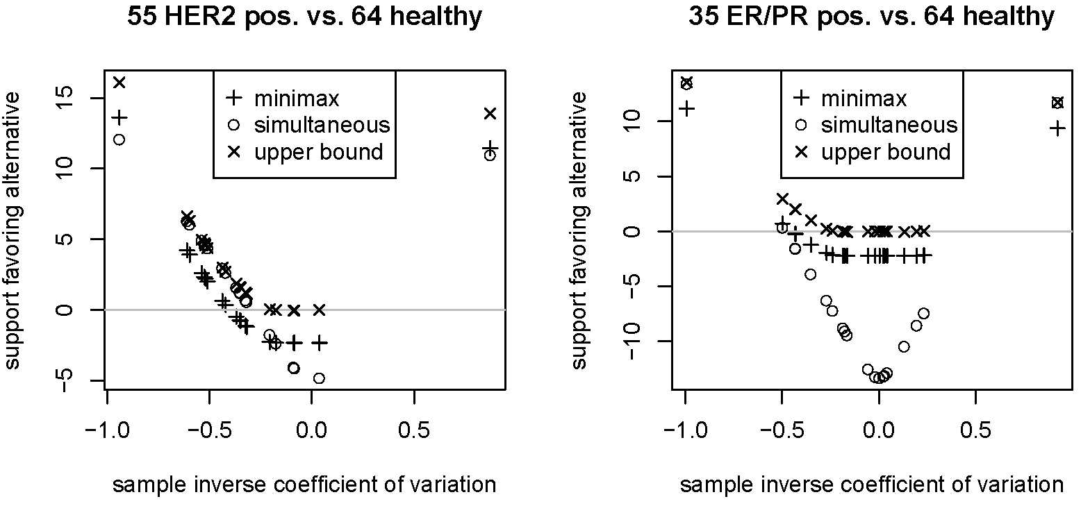
Figure 1: Single-comparison, sample-optimal support (“minimax”; $g_{1}^{\star}\left(t_{i}\right)/g_{0}\left(t_{i}\right)$) as an approximation to the estimated support that could be achieved with multiple comparisons (“simultaneous”; $g\left(t_{i}|\hat{\theta}_{\text{alternative}}\right)/g_{0}\left(t_{i}\right)$). The “upper bound” is $\max_{\theta\in\Theta}g\left(t_{i}|\theta\right)/g_{0}\left(t_{i}\right)$ (Bickel, 2010c), exceeding the optimal support by a constant amount.

6 Discussion

The proposed framework of evidential support may be viewed as an extension of likelihoodism, classically expressed in Edwards (1992), to nuisance parameters and multiple comparisons. Edwards (1992, §3.2) argued that a measure of evidence in data or support for one simple hypothesis (sampling distribution) over another should be compatible with Bayes’s theorem in the sense that whenever real-world parameter probabilities are available, the support quantifies the departure of posterior odds from prior odds. The likelihood ratio has that property, but the p-value does not since it only depends on the distribution of the null hypothesis. As compelling as the argument is for comparing two simple hypotheses, the pure likelihood approach does not apply to a composite hypothesis, a set of sampling distributions.

Perceiving the essential role of composite hypotheses in many applications, Zhang (2009) previously extended the likelihoodism by replacing the likelihood for the single distribution that represents a simple hypothesis with the likelihood maximized over all parameter values that constitute a composite hypothesis. Thus, the strength of evidence for the alternative hypothesis that $\phi$ is in some interval (or union of intervals) $\Phi_{1}$ over the null hypothesis that $\phi$ is in some other interval $\Phi_{0}$ would be $\max_{\phi\in\Phi_{1}}f\left(x_{i}|\phi\right)/\max_{\phi\in\Phi_{0}}f\left(x_{i}|\phi\right)$. For example, the strength of evidence favoring $\phi\neq\phi_{0}$ over $\phi=\phi_{0}$ would be $\max_{\phi\in\Phi}f\left(x_{i}|\phi\right)/f\left(x_{i}|\phi_{0}\right)$. The related approach of Bickel (2010c) performs the maximization after eliminating the nuisance parameter: $\max_{\theta\in\Theta}g\left(t_{i}|\theta\right)/g\left(t_{i}|\theta_{0}\right)$. While that approach to some extent justifies the use of likelihood intervals (Fisher, 1973) and has intuitive support from the principle of inference to the best explanation (Bickel, 2010c), it tends to overfit the data from a predictive viewpoint. For example, if $\theta_{1}=\arg\max_{\theta\in\Theta_{1}}L\left(\theta\right)$, then the evidence for the hypothesis that $\theta\in\Theta_{1}$ would be just as strong as the evidence for the hypothesis that $\theta=\theta_{1}$ even if the latter hypothesis were in primary view before observing $x$. Thus, the maximum likelihood ratio is considered as an upper bound of support in Fig. 1.

The present paper also generalizes the pure likelihood approach but without such overfitting. The proposed approach grew out of the Bayes-compatibility criterion of Edwards (1992). By leveraging recent advances in J. Rissanen’s information-theoretic approach to model selection, the Bayes-compatibility criterion was recast in terms of predictive distributions, thereby making support applicable to composite hypotheses. To qualify as a measure of support, a statistic must asymptotically mimic the difference between the posterior and prior log-odds, where the parameter distributions considered are physical in the empirical Bayes or random effects sense that they correspond to real frequencies or proportions (Robinson, 1991), whether or not the distributions can be estimated.

Generalized Bayes compatibility has advantages even when support is not used with a hypothetical prior probability. For example, defining support in terms of the difference between the posterior and prior log-odds (9) is sufficient for interpreting $S^{\star}\left(t_{i}\right)\geq 5$ or some other some level of support in the same way for any sample size (Royall, 2000b). In other words, no sample-size calibration is necessary (cf. Bickel, 2010b).

In addition to the Bayes-compatibility condition, an optimality criterion such as one of the two lifted from information theory is needed to uniquely specify a measure of support (§4). One of the resulting minimax-optimal measures of support performed well compared to the upper bound when applied to measured levels of a single protein (§5). The standard of comparison was the difference between posterior and prior log odds that could be estimated by simultaneously using the measurements of all 20 proteins. While both the minimax support and the upper bound come close to the simultaneous-inference standard, the conservative nature of the minimax support prevented it from overshooting the target as much as did the upper bound (Fig. 1). The discrepancy between the minimax support and the upper bound will become increasingly important as the dimension of the interest parameter increases. In high-dimensional applications, overfitting will render the upper bound unusable, but minimax support will be shielded by a correspondingly high penalty factor $\int_{\mathcal{T}}g\left(t;\hat{\theta}_{i}\left(t\right)\right)dt$ in equation (13).

References

- Berger and Pericchi (1996) Berger, J. O., Pericchi, L. R., 1996. The intrinsic Bayes factor for model selection and prediction. Journal of the American Statistical Association 91 (433), 109–122.
- Bickel (2010a) Bickel, D. R., 2010a. Minimum description length methods of medium-scale simultaneous inference. Technical Report, Ottawa Institute of Systems Biology, arXiv:1009.5981.
- Bickel (2010b) Bickel, D. R., 2010b. Statistical inference optimized with respect to the observed sample for single or multiple comparisons. Technical Report, Ottawa Institute of Systems Biology, arXiv:1010.0694.
- Bickel (2010c) Bickel, D. R., 2010c. The strength of statistical evidence for composite hypotheses: Inference to the best explanation. Technical Report, Ottawa Institute of Systems Biology, COBRA Preprint Series, Article 71, available at biostats.bepress.com/cobra/ps/art71.
- Blume (2002) Blume, J. D., 2002. Likelihood methods for measuring statistical evidence. Statistics In Medicine 21 (17), 2563–2599.
- Drmota and Szpankowski (2004) Drmota, M., Szpankowski, W., 2004. Precise minimax redundancy and regret. IEEE Transactions on Information Theory 50 (11), 2686–2707.
- Edwards (1992) Edwards, A. W. F., 1992. Likelihood. Johns Hopkins Press, Baltimore.
- Efron (2010a) Efron, B., 2010a. The future of indirect evidence. Statistical Science 25 (2), 145–157.
- Efron (2010b) Efron, B., 2010b. Large-Scale Inference: Empirical Bayes Methods for Estimation, Testing, and Prediction. Cambridge University Press.
- Efron et al. (2001) Efron, B., Tibshirani, R., Storey, J. D., Tusher, V., 2001. Empirical Bayes analysis of a microarray experiment. J. Am. Stat. Assoc. 96 (456), 1151–1160.
- Fisher (1973) Fisher, R. A., 1973. Statistical Methods and Scientific Inference. Hafner Press, New York.
- Gentleman et al. (2004) Gentleman, R. C., Carey, V. J., Bates, D. M., et al., 2004. Bioconductor: Open software development for computational biology and bioinformatics. Genome Biology 5, R80.
- Grünwald (2007) Grünwald, P. D., 2007. The Minimum Description Length Principle. The MIT Press, London.
- Hu and Zidek (2002) Hu, F. F., Zidek, J., 2002. The weighted likelihood. Canadian Journal of Statistics 30 (3), 347–371.
- Jeffreys (1948) Jeffreys, H., 1948. Theory of Probability. Oxford University Press, London.
- Kullback (1968) Kullback, S., 1968. Information Theory and Statistics. Dover, New York.
- Li (2009) Li, X., 2009. ProData. Bioconductor.org documentation for the ProData package.
- Qiu et al. (2005) Qiu, X., Klebanov, L., Yakovlev, A., 2005. Correlation between gene expression levels and limitations of the empirical Bayes methodology for finding differentially expressed genes. Statistical Applications in Genetics and Molecular Biology 4 (1), i–30.
- Rissanen (1987) Rissanen, J., 1987. Stochastic complexity. Journal of the Royal Statistical Society.Series B (Methodological) 49 (3), 223–239.
- Rissanen (2007) Rissanen, J., 2007. Information and Complexity in Statistical Modeling. Springer, New York.
- Rissanen (2009) Rissanen, J., 2009. Model selection and testing by the MDL principle. Information Theory and Statistical Learning. Springer, New York, Ch. 2, pp. 25–43.
- Robinson (1991) Robinson, G. K., 1991. That BLUP is a good thing: The estimation of random effects. Statistical Science 6 (1), 15–32.
- Royall (2000a) Royall, R., 2000a. On the probability of observing misleading statistical evidence. Journal of the American Statistical Association 95 (451), 760–768.
- Royall (2000b) Royall, R., 2000b. Rejoinder to comments on r. royall, "on the probability of observing misleading statistical evidence". Journal of the American Statistical Association 95 (451), 773–780.
- Shtarkov (1987) Shtarkov, Y. M., 1987. Universal sequential coding of single messages. Problems of information transmission 23 (3), 175–186.
- Wang and Zidek (2005) Wang, X., Zidek, J. V., 2005. Derivation of mixture distributions and weighted likelihood function as minimizers of KL-divergence subject to constraints. Annals of the Institute of Statistical Mathematics 57 (4), 687–701.
- Yang and Bickel (2010) Yang, Y., Bickel, D. R., 2010. Minimum description length and empirical Bayes methods of identifying snps associated with disease. Technical Report, Ottawa Institute of Systems Biology, COBRA Preprint Series, Article 74, available at biostats.bepress.com/cobra/ps/art74.
- Zhang (2009) Zhang, Z., 2009. A law of likelihood for composite hypotheses. arXiv:0901.0463.