Equilibrium and Stability of Polarization in Ultrathin Ferroelectric Films
with Ionic Surface Compensation

Abstract

Thermodynamic theory is developed for the ferroelectric phase transition of an ultrathin film in equilibrium with a chemical environment that supplies ionic species to compensate its surface. Equations of state and free energy expressions are developed based on Landau-Ginzburg-Devonshire theory, using electrochemical equilibria to provide ionic compensation boundary conditions. Calculations are presented for a monodomain PbTiO₃ (001) film coherently strained to SrTiO₃ with its exposed surface and its electronically conducting bottom electrode in equilibrium with a controlled oxygen partial pressure. The stability and metastability boundaries of phases of different polarization are determined as a function of temperature, oxygen partial pressure, and film thickness. Phase diagrams showing polarization and internal electric field are presented. At temperatures below a thickness-dependent Curie point, high or low oxygen partial pressure stabilizes positive or negative polarization, respectively. Results are compared to the standard cases of electronic compensation controlled by either an applied voltage or charge across two electrodes. Ionic surface compensation through chemical equilibrium with an environment introduces new features into the phase diagram. In ultrathin films, a stable nonpolar phase can occur between the positive and negative polar phases when varying the external chemical potential at fixed temperature, under conditions where charged surface species are not present in sufficient concentration to stabilize a polar phase.

I Introduction

The equilibrium polarization structure of an ultrathin ferroelectric film is strongly affected by the nature of the charge compensation of its interfaces. When there is insufficient free charge at the interfaces, a locally polar state can be stabilized by formation of equilibrium 180^∘ stripe domains that reduce the depolarizing field energy.02_StriefferPRL_89_067601 ; 04_Fong_Science ; GBS06JAP ; LAI07APL ; CT08APL ; BRAT08JCTN When electrodes are present, electronic charge at the interfaces can stabilize a monodomain polar state, provided that the effective screening length in the electrodes is sufficiently small compared with the film thickness.BRAT08JCTN ; BAT73PRL ; BAT73JVST ; WURF76FERRO ; DAWB03JPCM ; TAG06JAP ; JUNQ03NAT ; SAI05PRB ; 09_Stengel_NatMat In both cases, the Curie point $T_{C}$ is expected to be increasingly suppressed as film thickness decreases because of the residual depolarizing field energy.

Even when the surface electrode is missing, it has been experimentally observed that a monodomain polar state can be stable in ultrathin ferroelectric films.LICHT05PRL ; FONG06PRL ; 06_DespontPRB_73_094110 ; LICHT07APL This has been attributed to the presence of ionic species at the surface that provide charge compensation and reduce the depolarizing field energy,FONG06PRL similar to the adsorbates observed on bulk ferroelectric surfaces.06_KalininNL_4_555 Furthermore, experiments have shown that the sign of the polarization can be inverted by changing the chemical environment in equilibrium with the surface.09_WangPRL_102_047601 ; 10_Kim_APL96_202902 Recently10_HighlandPRL it was found that when the polarization is inverted by changing the external chemical potential, switching can occur without domain formation and at an internal field reaching the intrinsic coercive field for certain ranges of film thickness and temperature. Thus, through either kinetic suppression of domain nucleation, or the structure of the equilibrium phase diagram, an instability point of the initial polar state can be reached. This is in sharp contrast to switching by applied field across electrodes, where the consensus has been that polarization inversion occurs only by domain nucleation and growth at fields well below the instability.05_Dawber_RevModPhys77_1083

These studies motivate the need to understand the polarization phase diagrams and metastability limits for ultrathin ferroelectric films with ionic surface compensation, in chemical equilibrium with their environment. While the energy and structure of ferroelectric surfaces compensated by ions have been predicted by ab initio calculations,FONG06PRL ; 09_WangPRL_102_047601 ; 06_Spanier_NanoLett6_735 ; 09_ShinNL_9_3720 these zero-temperature results have been extrapolated to experimental temperatures using simple entropy estimates, and to date have not included the effects of interaction with the ferroelectric phase transition and $T_{C}$. Here we develop a thermodynamic theory for the ferroelectric phase transition of an ultrathin film in an environment that supplies ionic species to compensate the polarization discontinuity at the surface of the ferroelectric. We use an approach based on Landau-Ginzburg-Devonshire (LGD) theory for the ferroelectric material,GBS06JAP with boundary conditions that include both the depolarizing field effects that arise in ultrathin films and the creation of ionic surface charge through electrochemical equilibria. This new chemical boundary condition is based on a Langmuir adsorption isotherm for ions.96_Schmickler We develop an expression for the free energy of the system and use it to determine the equilibrium monodomain polarization states and their stability. For simplicity we do not include additional “intrinsic” surface effects or polarization gradients in the ferroelectric.Kretschmer We compare and contrast our model for ionic compensating charge controlled by an applied chemical potential with existing models for electronic compensating charge controlled by either an applied voltage or fixed charge, to elucidate how the present predictions for ionic compensation differ from prior work.

We find that the equilibrium phase diagram of a monodomain ferroelectric film as a function of temperature and chemical potential can have a different form than the standard phase diagrams as a function of temperature and applied voltage or charge. We present calculations for PbTiO₃ (001) films with a conducting bottom electrode (e.g., SrRuO₃), coherently strained to SrTiO₃, and with a surface compensated by excess or missing oxygen ions.FONG06PRL ; 09_WangPRL_102_047601 For sufficiently thin films, we find that a nonpolar state becomes stable between the positive and negative polar states, within the range of external oxygen partial pressures where there is insufficient surface charge to stabilize a polar state. Under these conditions the Curie temperature depends strongly on the oxygen chemical potential.

II Thermodynamic Model

In this section we establish the electrostatic boundary condition, the ferroelectric constitutive relation, and the free energy expressions used to describe an ultrathin ferroelectric film. We consider a uniformly polarized, monodomain film with uniaxial polarization oriented out-of-plane (normal to the interfaces). This should apply to systems such as PbTiO₃ (001) coherently strained to SrTiO₃, since LGD theoryGBS06JAP ; 01_Koukhar_PRB64_214103 predicts that compressive in-plane strain favors this “$c$ domain” polarization orientation. Even if out-of-plane polarization is suppressed by depolarization field effects, in this system the in-plane “$a$ domain” polarization orientation is less stable than the nonpolar phase10_HighlandPRL at temperatures above 360 K. For this case all fields can be specified by scalars since their in-plane components are zero.

To include the effects of incompletely neutralized depolarizing field, we use the simple electrostatic model illustrated in Fig. 1. The spatial separation between the compensating free charge in the electrodes and the bound charge at the outer surfaces of the ferroelectric leads to residual depolarizing field in the film even when the external voltage $V_{ex}$ is zero (i.e. short-circuit conditions). Figure 1 shows the polarization $P$ and displacement $D$ in a ferroelectric film of thickness $t$ sandwiched on the top and bottom by planes of compensating free charge of density $\pm\sigma$, at a distance $\lambda\geq 0$ outside the ferroelectric. The planes of bound and free charge lead to steps in $P$ and $D$, respectively. In Fig. 1, $P$ and $D$ are positive and the free charge on the top electrode $\sigma$ is negative. The electric field and potential can be calculated from $E=(D-P)/\epsilon_{0}$ and $\nabla\phi=-E$, where $\epsilon_{0}$ is the permittivity of free space. The internal field in the ferroelectric film is $E_{in}=-(\sigma+P)/\epsilon_{0}$, while the field just outside the film is $E_{\lambda}=-\sigma/\epsilon_{0}$.

In a series of early papers, Batra, Wurfel, and SilvermanBAT73PRL ; BAT73JVST ; WURF76FERRO showed that the results of a more complex model taking into account the space charge distribution and nonzero screening length in non-ideal metal electrodes could be reproduced by this simple model in which ideal metal electrodes are separated from the ferroelectric by a vacuum gap of width equal to the screening length, and all bound and free charges reside at the interfaces. This model has been discussed extensivelyBRAT08JCTN ; DAWB03JPCM ; LICHT05PRL ; TAG06JAP and used to parametrize the results of ab initio calculations.JUNQ03NAT An alternative description in terms of interfacial capacitance09_Stengel_NatMat ; 06_Stengel_Nature is equivalent if the interfacial capacitance per unit area is identified with $\epsilon_{0}/\lambda$. Recent calculationsSAI05PRB ; 09_Stengel_NatMat ; 09_StengelPRB_80_224110 have shown that the screening length for the electrode material can be generalized to be an effective screening length for a given ferroelectric/electrode interface.

Figure 1: Schematic of polarization, displacement, electric field, and electric potential in the bulk and at the interfaces of a ferroelectric film of thickness $t$ and polarization $P$. Compensating planes of charge density $\sigma$ can be considered to reside at a separation $\lambda$ equal to the effective screening length in the electrodes.

We can relate the external voltage $V_{ex}$ across the structure to $\sigma$ and $P$ by integrating the field to give

$$\epsilon_{0}V_{ex}=2\lambda\sigma+t(\sigma+P).$$ (1)

The field in the ferroelectric can then be expressed as a function of $P$ and either $\sigma$ or $V_{ex}$ using

$$E_{in} = -(\sigma+P)/\epsilon_{0}$$ (2)

$$= -\frac{V_{ex}+2\lambda P/\epsilon_{0}}{2\lambda+t}.$$

In the latter expression, the second term in the numerator gives the voltage from the residual depolarizing field that is proportional to (and opposes) the film polarization.

In this simple electrostatic model, we assume that the two interfaces have the same screening length and work function. In a polarized material, these quantities can depend upon the polarization magnitude and orientation with respect to the surface, and differences between the two interfaces may arise even if the electrode materials are identical.SAI05PRB ; 09_StengelPRB_80_224110 Since to first order these effects simply add a term to $2\lambda$ in the numerator of Eq. (2), which is already a variable parameter in our model, we have neglected these differences. The approximations in this electrostatic model are not critical in determining the new behaviors we find below for ionic surface compensation (which occur even for $\lambda=0$), but do provide simple, analogous electronic compensation models for comparison.

To determine the equilibrium polarization in the film, the values of field and polarization inside the ferroelectric must simultaneously satisfy both the electrostatic boundary condition Eq. (2) and the $E_{in}(P)$ constitutive relation for the ferroelectric. For PbTiO₃ this can be written asGBS06JAP

$$E_{in}=f^{\prime}(P)=2\alpha_{3}^{*}P+4\alpha_{33}^{*}P^{3}+6\alpha_{111}P^{5},$$ (3)

where $f^{\prime}(P)$ is the derivative of the bulk LGD free energy density

$$f(P)\equiv\alpha_{3}^{*}P^{2}+\alpha_{33}^{*}P^{4}+\alpha_{111}P^{6},$$ (4)

and the coefficients $\alpha_{i}^{*}$ are those for a coherently-strained film,98_PertsevPRL_80_1988

$$\alpha_{3}^{*} = \frac{T-T_{0}}{2\epsilon_{0}C}-\frac{2x_{m}Q_{12}}{s_{11}+s_{12}},$$

$$\alpha_{33}^{*} = \alpha_{11}+\frac{Q_{12}^{2}}{s_{11}+s_{12}},$$ (5)

where $x_{m}$ is the epitaxial misfit strain of the zero polarization state, $T_{0}$ is the temperature at which $\alpha_{3}^{*}$ changes sign for $x_{m}=0$, $C$ is the Curie constant, and $Q_{ij}$ and $s_{ij}$ are the electrostrictive and elastic compliance coefficients, respectively.GBS06JAP ; HAUN87JAP ; ROS98JMR Values of these material parameters for PbTiO₃ are listed in Table 1. The misfit strain $x_{m}$ has a somewhat temperature-dependent valueGBS06JAP of about -0.01 for PbTiO₃ coherently strained to SrTiO₃. While for unstressed bulk PbTiO₃ the fourth-order polarization coefficient $\alpha_{11}$ is slightly negative, indicating a weakly first-order transition as a function of $T$ at $E_{in}=0$, for coherently strained films the coefficient $\alpha_{33}^{*}$ has a positive value of $5.0\times 10^{7}$ Vm⁵/C³, indicating that the transition is second order.98_PertsevPRL_80_1988

The strain normal to the film can be calculated from the polarization using the expressionGBS06JAP

$$x_{3}=Q_{11}P^{2}+2s_{12}(x_{m}-Q_{12}P^{2})/(s_{11}+s_{12}).$$ (6)

If the effects of depolarizing field are neglected (i.e. for ideal electrodes with $\lambda=0$), the Curie temperature $T_{C}^{\circ}$ is determined by the change in sign of $\alpha_{3}^{*}$, which gives

$$T_{C}^{\circ}=T_{0}+4\epsilon_{0}CQ_{12}x_{m}/(s_{11}+s_{12}).$$ (7)

Using the $x_{m}(T)$ appropriate for epitaxially strained PbTiO₃ on SrTiO₃, this gives $T_{C}^{\circ}=1023$ K, about 270 K higher than in the $x_{m}=0$ case.

Table 1: Material parametersGBS06JAP ; HAUN87JAP ; ROS98JMR for PbTiO₃.

$T_{0}$	752.0	(K)	$Q_{11}$	$8.9\times 10^{-2}$	(m4/C2)
$C$	$1.5\times 10^{5}$	(K)	$Q_{12}$	$-2.6\times 10^{-2}$	(m4/C2)
$\alpha_{11}$	$-7.25\times 10^{7}$	(Vm5/C3)	$s_{11}$	$8.0\times 10^{-12}$	(m2/N)
$\alpha_{111}$	$2.61\times 10^{8}$	(Vm9/C5)	$s_{12}$	$-2.5\times 10^{-12}$	(m2/N)

We can determine which of the equilibrium solutions is stable, metastable, or unstable by considering the appropriate free energy of the system. For a closed system (e.g. fixed charge), the Helmholtz free energy is minimized at equilibrium. The Helmholtz free energy per unit area ${\cal A}$ can be written asGBS06JAP

$${\cal A} = t[f(P)+\frac{\epsilon_{0}}{2}E_{in}^{2}]+2\lambda\frac{\epsilon_{0}}{2}E_{\lambda}^{2}$$ (8)

$$= t\left[f(P)+\frac{(\sigma+P)^{2}}{2\epsilon_{0}}\right]+\frac{\lambda\sigma^{2}}{\epsilon_{0}},$$

where the two terms are for the ferroelectric film and surrounding screening regions. For an open system (e.g. fixed potential), the Gibbs free energy is minimized at equilibrium. The Gibbs free energy per unit area ${\cal G}$ is given byGBS06JAP

$${\cal G}={\cal A}-V_{ex}\sigma,$$ (9)

where the difference between the Gibbs and Helmholtz free energies $-V_{ex}\sigma$ is the electrical work done on the system by the external circuit. This difference is in accord with that in a recent derivation09_StengelNatPhys_5_304 of the energy functionals to be minimized in first-principles calculations at fixed $D$ and fixed $E$.

III Ferroelectric film with electronic compensation

In this section we present the equations of state and phase diagrams for ferroelectric films with electronic compensation under controlled voltage or charge conditions, as background for development of theory for ionic compensation. Some of the more subtle differences between fixed voltage and fixed charge boundary conditions are highlighted.

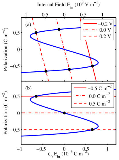
Figure 2: (Color online) Polarization vs. internal field. Straight red lines show (a) fixed $V_{ex}$ (at $t$ = 3.2 nm and $\lambda/t=10^{-4}$) or (b) fixed $\sigma$ boundary conditions from Eq. (2), for the three values of the fixed quantity given in the legend. In each case, the “S” shaped blue curve is the constitutive relation, Eq. (3), for PbTiO₃ coherently strained to SrTiO₃ at 644 K. Marked intersections correspond to stable or metastable equilibrium solutions.

Figure 2 graphically shows the equilibrium polarization and field values that simultaneously satisfy the constitutive relation, Eq. (3), and either the fixed $V_{ex}$ or the fixed $\sigma$ boundary condition. A temperature of 644 K was chosen to match one of the experimental conditions previously studied.09_WangPRL_102_047601 ; 10_HighlandPRL Each line in Fig. 2(a) is the fixed $V_{ex}$ boundary condition from the second equality of Eq. (2) for a particular value of $V_{ex}$. The deviation of this line from vertical reflects the nonzero value of $\lambda/t=10^{-4}$ used to model the screening length in the electrodes. As $V_{ex}$ is varied, this boundary condition translates along the horizontal $E_{in}$ axis. For $|V_{ex}|$ less than a certain value, there are three intersections representing equilibrium solutions; at larger $|V_{ex}|$, there is only a single solution. The marked intersections correspond to solutions that are not unstable, as described below. Each line in Fig. 2(b) is the fixed $\sigma$ boundary condition from the first equality of Eq. (2) for a particular value of $\sigma$. These lines are nearly horizontal, showing that the field dependence of $P$ at constant $\sigma$ is negligible. As $\sigma$ is varied, this boundary condition translates along the vertical $P$ axis. In this fixed, uniform $\sigma$ case, there is a single equilibrium solution at all $\sigma$ and $T$ values. The behavior is independent of $\lambda$ and $t$, and, as described below, the equilibrium solution is always stable.

III.1 Phase diagram for controlled $V_{ex}$

At constant $V_{ex}$, the equilibrium polarization value is that which minimizes ${\cal G}$. Using Eq. (1) to eliminate $\sigma$ gives an expression for ${\cal G}$ in terms of $V_{ex}$ and $P$,

$${\cal G}=tf(P)-\frac{\epsilon_{0}V_{ex}^{2}}{2(2\lambda+t)}+\frac{tPV_{ex}}{2\lambda+t}+\frac{\lambda tP^{2}}{\epsilon_{0}(2\lambda+t)}.$$ (10)

Figure 3 shows ${\cal G}$ as a function of $P$ and $V_{ex}$ corresponding to Fig. 2(a). The equilibrium polarization $P_{eq}$ can be determined by setting the first derivative of ${\cal G}$ at constant $V_{ex}$ to zero, giving the equation of state

$$0=\frac{1}{t}\left.\frac{\partial\cal G}{\partial P}\right|_{V_{ex}}=f^{\prime}(P)+\frac{V_{ex}+2\lambda P/\epsilon_{0}}{2\lambda+t}.$$ (11)

This agrees with the simultaneous solution of the constitutive relation and boundary condition shown above, Eqs. (2) and (3).

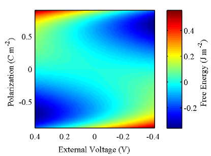
Figure 3: (Color online) Gibbs free energy ${\cal G}$ vs. $P$ and $V_{ex}$ for a $t=3.2$ nm PbTiO₃ film coherently strained to SrTiO₃ at 644 K, with $\lambda/t=10^{-4}$. Color scale gives values of ${\cal G}$.

The stability of the equilibrium solutions of Eq. (11) is determined by the sign of the second derivative of ${\cal G}$ at that value of $P$,

$$\frac{1}{t}\left.\frac{\partial^{2}\cal G}{\partial P^{2}}\right|_{V_{ex}}=f^{\prime\prime}(P)+\frac{2\lambda}{\epsilon_{0}(2\lambda+t)}.$$ (12)

When this is negative, the solution is unstable; when it is positive, the solution is stable or metastable. In particular, when there are three solutions, as shown in Fig. 2(a), the middle one near $P=0$ is unstable. The values of $P$ and $V_{ex}$ at the instability (limit of metastability) are given by the condition that both the first and second derivatives of ${\cal G}$ are zero. At this value of $P$, the $P(E_{in})$ curve of the constitutive equation, Eq. (3), has the same slope as the constant $V_{ex}$ boundary condition line, Eq. (2), in Fig. 2(a). The value of $E_{in}$ at the instability is the intrinsic coercive field for the film/electrode system with parameters $t$ and $\lambda$, taking into account the effect of depolarizing field.

The solution of Eq. (12) for $P=0$ gives the condition for the Curie temperature $T_{C}$ which can differ from the value $T_{C}^{\circ}$ for $\lambda=0$. The change in $T_{C}$ due to a nonzero screening length is given byBAT73JVST

$$\Delta T\equiv T_{C}-T_{C}^{\circ}=\frac{-2\lambda C}{2\lambda+t}.$$ (13)

Because the Curie constant $C$ is much larger than $T_{C}^{\circ}$ for typical ferroelectrics, stability of the polar phase requires $\lambda<<t$. Even a ratio $\lambda/t=0.001$ gives $\Delta T=-300$ K for PbTiO₃. Effective screening lengths $\lambda$ calculated from first principlesJUNQ03NAT ; 09_Stengel_NatMat vary between zero and 0.02 nm for various electrode-ferroelectric interfaces.

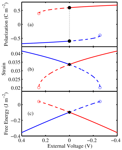
Figure 4: (Color online) Equilibrium solutions for (a) polarization $P$, (b) strain $x_{3}$, and (c) Gibbs free energy ${\cal G}$ as a function of $V_{ex}$, calculated for PbTiO₃ coherently strained to SrTiO₃ at 644 K with $t=3.2$ nm and $\lambda/t=10^{-4}$. Red (blue) curves are positive (negative) polarization; solid (dashed) segments are stable (metastable); closed (open) circles show equilibrium transition (instability) points.

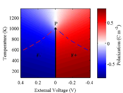
Figure 5: (Color online) Equilibrium polarization phase diagram as a function of $V_{ex}$ and $T$ for PbTiO₃ coherently strained to SrTiO₃ with $t=3.2$ nm and $\lambda/t=10^{-4}$. Color scale gives polarization of stable phase. Solid black line is phase boundary between positive and negative polar ferroelectric (F+ and F-) phases, terminating at $T_{C}$. Dashed red and blue curves are metastability limits of the F+ and F- phases, respectively.

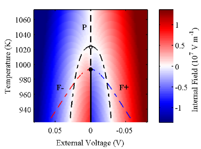
Figure 6: (Color online) Internal field in region near the Curie point, corresponding to Fig. 5. Color scale gives electric field in stable phase. Dashed black curves show conditions for zero field, which intersect at $T_{C}^{\circ}$ (open circle), the Curie point for a film without depolarizing field $(\lambda=0)$.

Figure 4 shows the equilibrium polarization, strain, and free energy of the stable and metastable solutions as a function of $V_{ex}$. These indicate the possible polarization hysteresis and strain butterfly loops. Two equilibrium solutions (one stable and one metastable) corresponding to oppositely polarized states exist when $|V_{ex}|$ is smaller than the instability. The stable solution switches between positive and negative polarization at $V_{ex}=0$. At values of $V_{ex}$ in the metastable region between the equilibrium and instability points, polarization switching requires nucleation of domains of the opposite polarity. The nucleation barrier becomes zero when $V_{ex}$ reaches the instability.CAHN59JCP At values of $V_{ex}$ exceeding the instability, switching occurs by a continuous process without nucleation.

Figure 5 shows the equilibrium polarization phase diagram as a function of $V_{ex}$ and $T$. While there is a first-order transition phase between positive and negative polar ferroelectric (F+ and F-) phases, this terminates at $T_{C}$ in a second-order transition to the nonpolar paraelectric (P) phaseStrukov98 . When $T$ is varied at nonzero values of $V_{ex}$, there is no phase transition between the nonpolar and the stable polar phase. The dashed red and blue curves are the limits of the metastable F+ and F- phases, respectively. The polarity switching transition driven by changing $V_{ex}$ at fixed $T$ requires nucleation under conditions inside (below) these curves, and is continuous (non-nucleated) outside (above) these curves.

The nonzero screening length $\lambda$ not only depresses $T_{C}$ below $T_{C}^{\circ}$, but also produces inverted electric fields in the film in the region near the phase boundary (small $|V_{ex}|$). Figure 6 shows the internal field as a function of $V_{ex}$ and $T$ in the vicinity of $T_{C}$. The inverted electric fields extend into the nonpolar phase in the region between $T_{C}$ and $T_{C}^{\circ}$. Thus, when a small external voltage is applied to a film in this region, the equilibrium field in the film is opposite to the applied field. Close to $T_{C}$, the magnitude of this inverted field is larger than that of the applied field, producing an (internal) voltage gain in a passive device that diverges as $T_{C}$ is approached. It has been proposed that such “negative capacitance” could be used to improve the performance of nanoscale transistors.Salahuddin08NL The conditions for zero field, shown as black dashed curves in Fig. 6, can be obtained from Eq. (2) as $V_{ex}=-(2\lambda/\epsilon_{0})P_{0}$, where $P_{0}$ is the zero-field spontaneous polarization of the epitaxially strained film.GBS06JAP Unlike $T_{C}$, these boundaries are independent of film thickness.

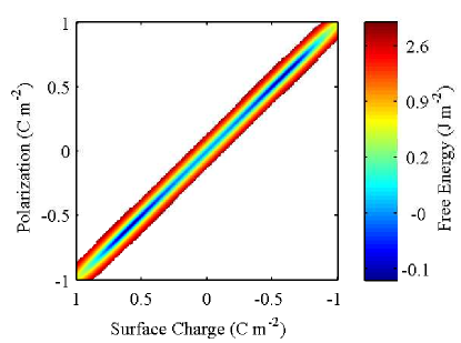
Figure 7: (Color online) Helmholtz free energy ${\cal A}$ vs. polarization $P$ and surface charge $\sigma$ for a $t=3.2$ nm PbTiO₃ film coherently strained to SrTiO₃ at 644 K, with $\lambda/t=10^{-4}$. Color scale gives values of ${\cal A}$. To emphasize the equilibrium solutions, only the region near $P=-\sigma$ is plotted since ${\cal A}$ is very large outside this region.

III.2 Phase diagram for controlled $\sigma$

An alternative to controlling the voltage $V_{ex}$ across the electrodes is to control the current flow to the electrodes, and hence the free charge $\sigma$. The equilibrium polarization at fixed $\sigma$ is determined by minimizing the Helmholtz free energy for the system given by Eq. (8). This is plotted as a function of $P$ and $\sigma$ in Fig. 7. Setting to zero the derivative of $\cal A$ at constant $\sigma$ gives the equation of state

$$0=\frac{1}{t}\left.\frac{\partial\cal A}{\partial P}\right|_{\sigma}=f^{\prime}(P)+\frac{\sigma+P}{\epsilon_{0}}.$$ (14)

This agrees with the constitutive relation, Eq. (3), verifying that the correct equilibrium states are predicted by this free energy for fixed $\sigma$. Since $C/T_{C}^{\circ}$ is very large for typical ferroelectrics, there is a only one minimum at each value of $\sigma$. The equilibrium values of $\cal A$ and $V_{ex}$ are plotted versus $\sigma$ in Fig. 8. To a good approximation, this equilibrium solution corresponds to $P_{eq}\approx-\sigma$, and

$${\cal A}_{eq} \approx tf(\sigma)+\frac{\lambda\sigma^{2}}{\epsilon_{0}},$$

$$V_{ex}^{eq} \approx tf^{\prime}(\sigma)+2\lambda\frac{\sigma}{\epsilon_{0}}.$$ (15)

If these approximate expressions were plotted with the exact results in Fig. 8, the curves would be indistinguishable.

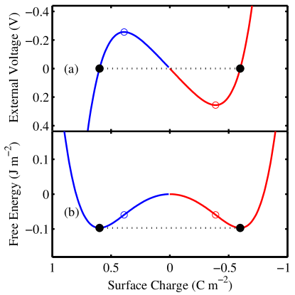
Figure 8: (Color online) Equilibrium solutions for (a) external voltage $V_{ex}$ and (b) Helmholtz free energy ${\cal A}$ as a function of surface charge $\sigma$ corresponding to Fig. 7. Red (blue) curves are positive (negative) polarization; all values are stable with respect to $P$ variations when $\sigma$ is spatially uniform. Closed (open) circles show the equilibrium transition (instability) points when $\sigma$ can be nonuniform.

The stability of this equilibrium solution with respect to variations in $P$ can be evaluated from the sign of the second derivative of ${\cal A}$ with respect to $P$,

$$\frac{1}{t}\left.\frac{\partial^{2}\cal A}{\partial P^{2}}\right|_{\sigma}=f^{\prime\prime}(P)+\frac{1}{\epsilon_{0}}.$$ (16)

Because $C/T_{C}$ is very large, the first term is negligible, and the second derivative is always positive. Unlike the fixed $V_{ex}$ case, the equilibrium solution $P_{eq}\approx-\sigma$ is never unstable with respect to fluctuations in $P$, and there is no phase transition. This point is often not recognized – if the surface charge is controlled and kept uniform, any value of $P$ in the film may be stably formed.

While at fixed surface charge density $\sigma$ the equilibrium solution is always stable with respect to polarization variations, instability can occur with respect to spatial nonuniformity in $\sigma$. The free energy ${\cal A}_{eq}$ of Eq. (15) is a double well, as shown in Fig. 8(b). The minima occur at values $\sigma_{min}$ given by solutions of

$$0=\frac{1}{t}\frac{d{\cal A}_{eq}}{d\sigma}\approx f^{\prime}(\sigma)+\frac{2\lambda\sigma}{t\epsilon_{0}}.$$ (17)

This gives $V_{ex}^{eq}(\sigma_{min})=0$. If the controlled parameter is the net charge density on the electrode ${\bar{\sigma}}$, then for $|{\bar{\sigma}}|<|\sigma_{min}|$ the system can lower its free energy by forming a two-phase mixture of domains of opposite polarity. The extent of this two-phase region is shown by the black dotted lines in Fig. 8. The local surface charge $\sigma=\pm|\sigma_{min}|$ will have opposite sign for oppositely polarized domains. At equilibrium, the fraction of positive domains $x_{pos}$ will be $x_{pos}=(1-{\bar{\sigma}}/|\sigma_{min}|)/2$. The equilibrium value of $V_{ex}$ is zero in this polydomain region and the free energy densities of the oppositely polarized domains are equal.

Here we assume that the in-plane size of the domains is sufficiently large compared with the film thickness that we can neglect the excess free energy of the domain walls and the in-plane components and nonuniformity of the polarization and field near the domain walls. When there is incomplete neutralization of the depolarizing field by compensating charge (e.g. when $\lambda$ is not zero), the free energy can in some cases be reduced by the formation of equilibrium 180^∘ stripe domains02_StriefferPRL_89_067601 ; GBS06JAP ; BRAT08JCTN with an in-plane size similar to or less than the film thickness. For such fine-scale domain structures, the domain wall energies and field variations are not negligible. For simplicity, we do not consider these cases here.

The surface charge density is a conserved order parameter, so instability with respect to spatial nonuniformity occurs for magnitudes of $\sigma$ smaller than the spinodal values given by

$$0=\frac{1}{t}\frac{d^{2}{\cal A}_{eq}}{d\sigma^{2}}\approx f^{\prime\prime}(\sigma)+\frac{2\lambda}{t\epsilon_{0}}.$$ (18)

Since $\lambda<<t$, this expression gives the same result as the instability with respect to uniform $P$ variations at constant $V_{ex}$, Eq. (12).

Figure 9 shows the equilibrium polarization phase diagram as a function of ${\bar{\sigma}}$ and $T$, while Fig. 10 shows the internal field in the vicinity of $T_{C}$. These exhibit a two-phase field between the single-phase positive and negative polar phases (F+ and F-). The dashed red and blue spinodal curves are the metastability limits of the F+ and F- phases, respectively. The polarization behavior is especially simple, since we have $P\approx-\sigma$ in the single-phase regions, independent of $T$. The suppression of $T_{C}$ is the same as in the controlled $V_{ex}$ case, and the equilibrium and instability curves correspond exactly. However, transformations driven by controlling either $V_{ex}$ or ${\bar{\sigma}}$ follow different paths. If $V_{ex}$ is kept constant, the parent phase will remain metastable and will be entirely consumed by the stable phase. If ${\bar{\sigma}}$ is kept constant, $V_{ex}$ will decrease to zero as the fraction of inverted domains grows, reaching an equilibrium two-phase state. The controlled potential and controlled charge phase diagrams for ferroelectrics, Figs. 5 and 9, are directly analogous to controlled chemical potential and controlled composition phase diagrams for an alloy or fluid exhibiting phase separation.CAHN59JCP In particular, the instability in ferroelectrics is a spinodal boundary, and the continuous transition that occurs at fixed $V_{ex}$ in the unstable region is equivalent to spinodal decomposition of an alloy held at constant chemical potential. In this case, unlike the usual fixed average composition constraint for an alloy, the continuous transition will result in a single-phase (monodomain) final state. Spinodal transitions from monodomain to polydomain states in ferroelectrics at fixed ${\bar{\sigma}}$ have recently been modeled.ARTEMEV10AM

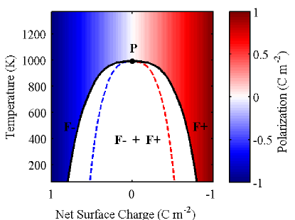
Figure 9: (Color online) Equilibrium phase diagram as a function of net surface charge ${\bar{\sigma}}$ and $T$ when $\sigma$ can be nonuniform, for PbTiO₃ coherently strained to SrTiO₃ with $t=3.2$ nm and $\lambda/t=10^{-4}$. Color scale gives polarization in single-phase region. Solid black line is phase boundary between positive and negative polar ferroelectric (F+ and F-) phases and a two-phase field, which terminates at $T_{C}$ (filled circle). Dashed red and blue curves are metastability limits of the F+ and F- phases, respectively.

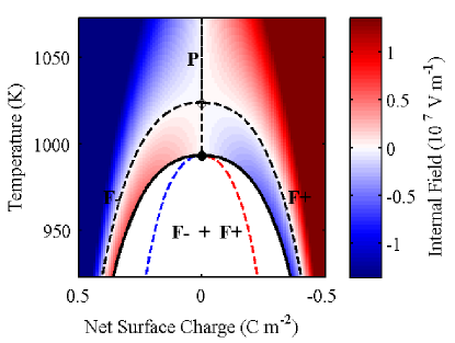
Figure 10: (Color online) Internal field in the region near the Curie point, corresponding to Fig. 9. Color scale gives electric field in single-phase region. Dashed black curves show conditions for zero field.

While the conclusion that the $P\approx-\sigma$ solution is always stable with respect to $P$ fluctuations for any constant $\sigma$ may seem practically irrelevant for the electronic compensation case where the system is unstable with respect to $\sigma$ nonuniformity, in the case of ionic compensation this conclusion can be important. As we shall see, for ionic compensation the system can be stable against $\sigma$ nonuniformity, and the phase transition to a polar state can be completely suppressed for a range of applied chemical potential.

IV Ferroelectric film with ionic surface compensation

Now we consider a ferroelectric film without a top electrode, but with its surface exposed to a chemical environment that can supply free charge from ionic species. The amount of free charge supplied will depend on the chemical composition of the environment and the external voltage $V_{ex}$ that it sees on the surface. We will use the same electrostatic boundary condition, Eq. (1), constitutive relation, Eq. (3), and free energy, Eq. (8), employed above for the electronic compensation cases, treating the ions as residing in a plane at a distance $\lambda$ above the surface. Rather than solving for the polarization for a given value of $V_{ex}$ or $\sigma$, we wish to obtain the equilibrium polarization for a given composition of the environment.

To obtain the relationship between $\sigma$ and $V_{ex}$ due to this chemical equilibrium, we develop an expression based on those for adsorption of ions used in electrochemical systems.96_Schmickler We treat the external chemical environment as an electrolyte that is in contact with both the surface of the film and the bottom electrode (e.g. via pinholes in the film away from the region of interest). In order for surface ions from the chemical environment to produce an electric field across the sample, as observed in experiments,09_WangPRL_102_047601 ; 10_Kim_APL96_202902 ; 10_HighlandPRL the electrons involved in creating the surface ions must have such a path to reach the bottom electrode.

We can write a generalized surface redox reaction between oxygen in the environment and a particular surface ion $i$,

$${\rm IonSite}+\frac{1}{n_{i}}{\rm O}_{2}\leftrightarrow z_{i}e^{-}+{\rm Ion}^{z_{i}},$$ (19)

where $n_{i}$ is the number of surface ions created per oxygen molecule, and $z_{i}$ is the charge on the surface ion. In this formalism, $n_{i}$ and $z_{i}$ change sign depending upon whether positively or negatively charged surface species are involved. For example, if the surface ion is a doubly-negatively-charged single-atom adsorbed oxygen, ${\rm O}_{ad}^{2-}$, so that $n_{i}=2$ and $z_{i}=-2$, the redox reaction is

$${\rm V}_{ad}+\frac{1}{2}{\rm O}_{2}+2e^{-}\leftrightarrow{\rm O}_{ad}^{2-},$$ (20)

while if the surface ion is a doubly-positively-charged single-atom missing surface oxygen, ${\rm V}_{O}^{2+}$, so that $n_{i}=-2$ and $z_{i}=2$, the redox reaction is

$${\rm O}_{O}\leftrightarrow\frac{1}{2}{\rm O}_{2}+2e^{-}+{\rm V}_{O}^{2+}.$$ (21)

In these reactions ${\rm V}_{ad}$ represents a vacant oxygen ion adsorption site on top of the film and ${\rm O}_{O}$ represents an occupied oxygen site in the outermost layer of the film. We include these sites in the equilibrium so that the concentration of ions saturates when all sites in the relevant surface layer are filled. The concentrations of surface ions, $\theta_{i}\equiv[{\rm Ion}]$, are defined so that their saturation levels are $\theta_{i}=1$ and the concentrations of the surface sites are $[{\rm IonSite}]=1-\theta_{i}$.

One can write mass-action equilibria for these redox reactions, taking into account the external voltage difference between the bottom electrode and the surface (since the electrons are assumed to reside at the bottom electrode, while the ions reside at the surface). These are given by

$$\frac{\theta_{i}}{1-\theta_{i}}=p_{O_{2}}^{1/n_{i}}\exp\left(\frac{-\Delta G_{i}^{\circ}-z_{i}eV_{ex}}{kT}\right),$$ (22)

where $\Delta G_{i}^{\circ}$ is the standard free energy of formation of the surface ion at $p_{O_{2}}=1$ bar and $V_{ex}=0$, and $e$ is the magnitude of the electron charge. This expression is analogous to the Langmuir adsorption isotherm used in interfacial electrochemistry96_Schmickler for adsorption of neutral species onto a conducting electrode exposed to ions in a solution. Here, we consider adsorption of ions onto a polar surface exposed to neutral species in a chemical environment. Thus our $V_{ex}$ is the potential of the adsorbed ions relative to the electrons, rather than the potential of the electrons relative to the ions in solution as in the typical electrochemical case.

The standard free energies can depend not only on temperature but also on the polarization of the film, since the surface structure changes with $P$. For simplicity we assume that they can be all described by the same parameter $\lambda^{\prime}$ using

$$\Delta G_{i}^{\circ} \equiv \Delta G_{i}^{\circ\circ}(T)+(z_{i}e\lambda^{\prime}/\epsilon_{0})P.$$ (23)

If $\lambda^{\prime}$ is positive, then a more positively polarized film tends to stabilize negative surface ions, and vice versa. Note that the effect of $\lambda^{\prime}$ is in addition to the electrostatic energy already included through the $z_{i}eV_{ex}$ term in Eq. (22). The density of free charge on the surface is the sum of those from the various surface ions, giving

$$\sigma=\sum_{i}\frac{z_{i}e\theta_{i}}{A_{i}},$$ (24)

where the $A_{i}^{-1}$ are the saturation densities of the surface ions.

Table 2: Values of ionic surface compensation coefficients used in displayed plots.

$\Delta G_{\oplus}^{\circ\circ}$	1.00	(eV)	$\Delta G_{\ominus}^{\circ\circ}$	0.00	(eV)
$n_{\oplus}$	$-2$		$n_{\ominus}$	$2$
$z_{\oplus}$	$2$		$z_{\ominus}$	$-2$
$A_{\oplus}$	$1.6\times 10^{-19}$	(m2)	$A_{\ominus}$	$1.6\times 10^{-19}$	(m2)
$\lambda$	0	(m)	$\lambda^{\prime}$	0	(m)

Using Eqs. (22)-(24) and Eq. (1), the surface ion concentrations $\theta_{i}$ can be calculated for given $V_{ex}$ and $p_{O_{2}}$. Parameter values for a system with one positive surface ion $i=\oplus$ and one negative surface ion $i=\ominus$ are given in Table 2; here $\Delta G_{\oplus}^{\circ\circ}$ and $\Delta G_{\ominus}^{\circ\circ}$ are taken to be independent of temperature. We have assumed that the saturation densities of the surface ions $A_{i}^{-1}$ are both one per PbTiO₃ unit cell area. For divalent surface ions, this saturation density would provide more than twice the charge density needed to fully compensate the typical polarization of PbTiO₃.

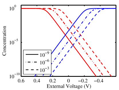
Figure 11: (Color online) Concentrations of positive $\theta_{\oplus}$ (red curves) and negative $\theta_{\ominus}$ (blue curves) surface ions as a function of $V_{ex}$, calculated for the values of $p_{O_{2}}$ (bar) given in the legend at $T=644$ K, $t=3.2$ nm. Parameter values used are given in Table 2.

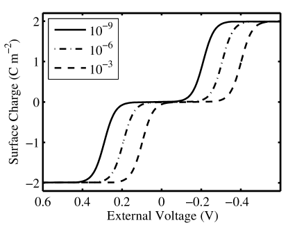
Figure 12: Surface charge density $\sigma$ as a function of $V_{ex}$ at three values of $p_{O_{2}}$, corresponding to the concentrations shown in Fig. 11. Parameter values used are given in Table 2.

Figure 11 shows $\theta_{i}$ as a function of $V_{ex}$ for several different values of $p_{O_{2}}$. Changing $p_{O_{2}}$ shifts the external voltage scale by $[kT/(z_{i}n_{i}e)]\Delta\ln p_{O_{2}}$ for each ion. Figure 12 shows the corresponding surface charge density $\sigma$. Three plateaus occur – two at extreme values of $V_{ex}$, where one or the other of the ionic surface concentrations $\theta_{i}$ saturates at unity, and a third near zero surface charge over the range of $V_{ex}$ for which both $\theta_{i}$ are small compared to unity. From the shape of the charge vs. voltage curves in Fig. 12, one can see that this fixed $p_{O_{2}}$ boundary condition has regions that correspond to fixed $\sigma$ separated by regions that correspond approximately to fixed $V_{ex}$. Thus fixed $p_{O_{2}}$ does not correspond to either fixed $\sigma$ or fixed $V_{ex}$. As we shall see, this strongly affects the equilibrium phase diagram.

The values of $p_{O_{2}}$ and $V_{ex}$ that give $\sigma=0$ can be obtained by solving Eqs. (22)-(24) for $\sigma=P=0$, $\theta_{i}<<1$, to give

$$\ln\left(\frac{p_{O_{2}}}{p^{\circ\circ}_{O_{2}}}\right)=\frac{n_{\ominus}n_{\oplus}(z_{\oplus}-z_{\ominus})}{n_{\ominus}-n_{\oplus}}\frac{eV_{ex}}{kT},$$ (25)

where $p^{\circ\circ}_{O_{2}}$ is the temperature-dependent oxygen partial pressure that gives $\sigma=P=0$ at $V_{ex}=0$,

$$\ln p^{\circ\circ}_{O_{2}}\equiv\frac{-n_{\ominus}n_{\oplus}}{n_{\ominus}-n_{\oplus}}\left[\frac{\Delta G_{\ominus}^{\circ\circ}-\Delta G_{\oplus}^{\circ\circ}}{kT}+\ln\left(\frac{z_{\oplus}A_{\ominus}}{-z_{\ominus}A_{\oplus}}\right)\right].$$ (26)

As shown below, this value of $p_{O_{2}}$ marks the transition between oppositely polarized films on the phase diagram.

IV.1 Equilibrium solutions at controlled oxygen partial pressure

Equilibrium solutions can be calculated by obtaining a relationship between $E_{in}$ and $P$ due to the fixed $p_{O_{2}}$ chemical boundary condition, and solving it simultaneously with the constitutive relation for the ferroelectric, as we did for the electronic case in Fig. 2. The solution for $\sigma$ as a function of $V_{ex}$ shown in Fig. 12 along with Eqs. (1) and (2) gives a relation between $E_{in}$ and $P$ for a given $p_{O_{2}}$, which can be solved simultaneously with Eq. (3) to obtain the overall equilibrium. This is illustrated in Fig. 13, where the chemical boundary condition for three values of $p_{O_{2}}$ is shown. Changing $p_{O_{2}}$ shifts the boundary condition curve along the $E_{in}$ axis. The boundary condition curve is centered on $P=0$, $E_{in}=0$ when $p_{O_{2}}$ is equal to $p^{\circ\circ}_{O_{2}}$ of Eq. (25).

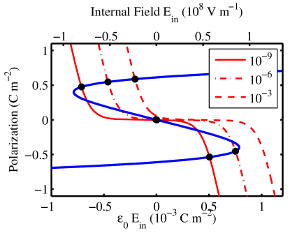
Figure 13: (Color online) Polarization vs. internal field relationships arising from the constitutive relation for the ferroelectric film (blue “S” shaped curve) and from the chemical boundary condition (red curves with plateau) for $p_{O_{2}}$ values shown in legend (bar). Marked intersections correspond to stable or metastable equilibrium solutions. Parameter values used are given in Tables 1 and 2, with $T=644$ K, $t=3.2$ nm.

An approximate expression for the chemical boundary condition can be obtained by making some simplifying assumptions. The dependence of $\sigma$ on $V_{ex}$ obtained from the depolarizing field, Eq. (1), is negligible compared with that obtained from the chemical equilibria, Eq. (24), shown in Fig. 12. One can approximate Eq. (1) as $\sigma\approx-P$. In addition, we can neglect one of the ion concentrations $\theta_{\oplus}$ or $\theta_{\ominus}$ relative to the other, depending on the sign of the film polarization. This leads to the limiting expressions

$$V_{ex}\approx-\frac{kT}{z_{i}e}\ln\frac{-A_{i}P/z_{i}e}{1+A_{i}P/z_{i}e}-\frac{\Delta G_{i}^{\circ\circ}}{z_{i}e}-\frac{\lambda^{\prime}}{\epsilon_{0}}P+\frac{kT\ln p_{O_{2}}}{z_{i}n_{i}e},$$ (27)

for $i=\ominus$ or $\oplus$ (positive or negative film polarization, respectively). For the parameters used in Fig. 12, e.g. far below $T_{C}$, the approximation (27) is very close to the exact solution obtained numerically. Substituting the approximation (27) into Eq. (2), one obtains relationships between field and polarization given by

$$\epsilon_{0}E_{in}\approx\frac{\epsilon_{0}(\frac{kT}{z_{i}e}\ln\frac{-A_{i}P/z_{i}e}{1+A_{i}P/z_{i}e}+\frac{\Delta G_{i}^{\circ\circ}}{z_{i}e}-\frac{kT\ln p_{O_{2}}}{z_{i}n_{i}e})-2\lambda^{\dagger}P}{2\lambda+t},$$ (28)

for $i=\ominus$ or $\oplus$. Here we have introduced a new parameter, $\lambda^{\dagger}$, defined by

$$\lambda^{\dagger}\equiv\lambda-\lambda^{\prime}/2.$$ (29)

If $\lambda^{\prime}$ is positive then $\lambda^{\dagger}$ is smaller than $\lambda$, and in particular $\lambda^{\dagger}$ can be negative.

IV.2 Stability of equilibrium solutions

Because of the plateau in the $P(E_{in})$ shape of the chemical boundary condition shown in Fig. 13, there can be as many as five equilibrium solutions given by the intersections. A total free energy function that is minimized at equilibrium can be used to determine which solutions are stable, metastable, and unstable. The Gibbs free energy consistent with the above treatment of ionic surface compensation is

$${\cal G} = t\left[f(P)+\frac{(\sigma+P)^{2}}{2\epsilon_{0}}\right]+\frac{\lambda^{\dagger}\sigma^{2}}{\epsilon_{0}}$$ (30)

$$+ \sum_{i=\ominus,\oplus}\frac{kT}{A_{i}}\left[\frac{\theta_{i}\Delta G_{i}^{\circ\circ}}{kT}-\frac{\theta_{i}\ln p_{O_{2}}}{n_{i}}\right.$$

$$+ \biggl{.}\theta_{i}\ln\theta_{i}+(1-\theta_{i})\ln(1-\theta_{i})\biggr{]}.$$

Minimizing this ${\cal G}$ with respect to $P$ at constant $p_{O_{2}}$, $\theta_{\ominus}$, and $\theta_{\oplus}$ (and therefore constant $\sigma$) gives

$$0=\frac{1}{t}\left.\frac{\partial{\cal G}}{\partial P}\right|_{\theta_{\oplus},\theta_{\ominus},p_{O_{2}}}=f^{\prime}(P)+\frac{\sigma+P}{\epsilon_{0}}.$$ (31)

This agrees with the constitutive relation, Eq. (3), like the case for electronic compensation, Eq. (14). As in that case, because of the large value of $C/T_{C}$ for PbTiO₃, the equilibrium polarization is given to a good approximation by $P\approx-\sigma$. The free energy expression then becomes

$${\cal G} \approx tf(\sigma)+\frac{\lambda^{\dagger}\sigma^{2}}{\epsilon_{0}}$$ (32)

$$+ \sum_{i=\ominus,\oplus}\frac{kT}{A_{i}}\left[\frac{\theta_{i}\Delta G_{i}^{\circ\circ}}{kT}-\frac{\theta_{i}\ln p_{O_{2}}}{n_{i}}\right.$$

$$+ \biggl{.}\theta_{i}\ln\theta_{i}+(1-\theta_{i})\ln(1-\theta_{i})\biggr{]}.$$

When the derivatives of this free energy with respect to $\theta_{\oplus}$ and $\theta_{\ominus}$ at fixed $p_{O_{2}}$ are set to zero, this yields the equilibrium relations given above in Eqs. (22-24), where $V_{ex}$ of Eq. (1) is now given by $V_{ex}\approx 2\lambda\sigma/\epsilon_{0}+tf^{\prime}(\sigma)$.

The global minimum of the free energy ${\cal G}$ of Eq. (32) with respect to $\theta_{\ominus}$ and $\theta_{\oplus}$ typically occurs either at $\theta_{\ominus}\approx 0$ or $\theta_{\oplus}\approx 0$. The generality of this result can be evaluated by re-expressing the $\theta_{\ominus}$ and $\theta_{\oplus}$ terms in the free energy Eq. (32) using new variables $\sigma$ and $\delta\equiv z_{\oplus}e\theta_{\oplus}/A_{\oplus}-z_{\ominus}e\theta_{\ominus}/A_{\ominus}$. Minimizing ${\cal G}$ with respect to $\delta$ at fixed $\sigma$ gives

$$0 = 2e\left.\frac{\partial{\cal G}}{\partial\delta}\right|_{\sigma,p_{O_{2}}}=\left(\frac{\Delta G_{\oplus}^{\circ\circ}}{z_{\oplus}}-\frac{\Delta G_{\ominus}^{\circ\circ}}{z_{\ominus}}\right)$$ (33)

$$+ \left[\frac{kT}{z_{\oplus}}\ln\left(\frac{\theta_{\oplus}}{1-\theta_{\oplus}}\right)-\frac{kT}{z_{\ominus}}\ln\left(\frac{\theta_{\ominus}}{1-\theta_{\ominus}}\right)\right]$$

$$+ \left(\frac{z_{\oplus}n_{\oplus}-z_{\ominus}n_{\ominus}}{z_{\oplus}n_{\oplus}z_{\ominus}n_{\ominus}}\right)kT\ln p_{O_{2}}.$$

The first term is positive in cases such as the one we consider, when there is a region of intermediate $p_{O_{2}}$ with low concentrations of both positive and negative surface ions. The third term is zero for typical values of the $z_{i}$ and $n_{i}$. Thus the equilibrium condition requires that the second term be negative, which occurs only when either $\theta_{\ominus}$ or $\theta_{\oplus}$ is very small. Substituting this result into Eq. (32) gives

$${\cal G} \approx tf(\sigma)+\frac{\lambda^{\dagger}\sigma^{2}}{\epsilon_{0}}+\frac{\sigma}{z_{i}e}\left(\Delta G_{i}^{\circ\circ}-\frac{kT\ln p_{O_{2}}}{n_{i}}\right)$$

$$+ \frac{kT}{A_{i}}\left[\frac{A_{i}\sigma}{z_{i}e}\ln\left(\frac{A_{i}\sigma}{z_{i}e}\right)+\left(1-\frac{A_{i}\sigma}{z_{i}e}\right)\ln\left(1-\frac{A_{i}\sigma}{z_{i}e}\right)\right],$$

where $i=\ominus$ for $\theta_{\oplus}\approx 0$, positive $P$, and negative $\sigma$, or $i=\oplus$ for $\theta_{\ominus}\approx 0$, negative $P$, and positive $\sigma$. The third term is proportional to $\sigma$, like a field term, but the constant of proportionality changes when $\sigma$ changes sign and the ionic species at the surface change between positive and negative ions. This change in slope of ${\cal G}(\sigma)$ at $\sigma=0$ can produce a stable or metastable minimum.

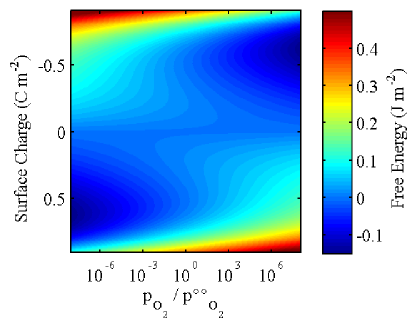
Figure 14: (Color online) Free energy as a function of $\sigma$ and $p_{O_{2}}/p^{\circ\circ}_{O_{2}}$. Parameter values used are given in Tables 1 and 2, with $T=644$ K, $t=3.2$ nm. Color scale gives values of ${\cal G}$.

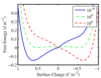
Figure 15: (Color online) Free energy as a function of $\sigma$ at three given values of $p_{O_{2}}/p^{\circ\circ}_{O_{2}}$. Parameter values used are given in Tables 1 and 2, with $T=644$ K, $t=3.2$ nm.

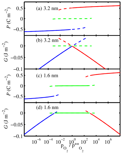
Figure 16: (Color online) Polarization $P$ and free energy ${\cal G}$ of the (meta-)stable equilibrium solutions as a function of $p_{O_{2}}/p^{\circ\circ}_{O_{2}}$. Blue, green, and red curves are for negative, zero, and positive polarization solutions; solid and dashed regions are stable and metastable, respectively. Parameter values used are given in Tables 1 and 2, with $T=644$ K, and $t=3.2$ nm for plots (a) and (b), $t=1.6$ nm for plots (c) and (d).

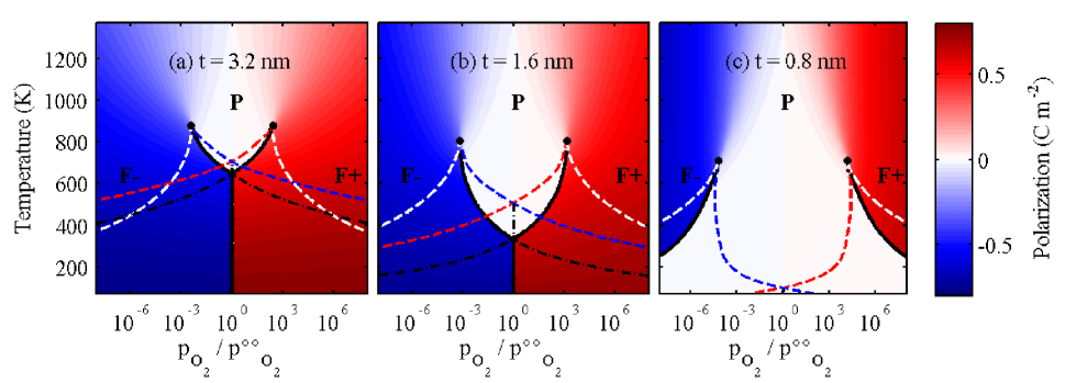
Figure 17: (Color online) Phase diagrams as a function of $p_{O_{2}}/p^{\circ\circ}_{O_{2}}$ and $T$ for three thicknesses of PbTiO₃ coherently strained to SrTiO₃, using parameters in Tables 1 and 2. Color scale gives polarization. Solid and dash-dot black curves are stable and metastable phase boundaries, respectively, between nonpolar paraelectric (P) and positive and negative polar ferroelectric (F+ and F-) phases. Dashed red, blue, and white curves are metastability limits of the F+, F-, and P phases, respectively.

The free energy of Eq. (IV.2) is plotted versus $p_{O_{2}}/p^{\circ\circ}_{O_{2}}$ and $\sigma$ in Figs. 14 and 15. At intermediate values of $p_{O_{2}}$, there are three (meta-)stable solutions corresponding to local minima in ${\cal G}(\sigma)$, at positive, zero, and negative polarization. These equilibrium solutions satisfy the equations of state

$$0 = \frac{\partial{\cal G}}{\partial\sigma}\approx tf^{\prime}(\sigma)+\frac{2\lambda^{\dagger}\sigma}{\epsilon_{0}}+\frac{1}{z_{i}e}\left(\Delta G_{i}^{\circ\circ}-\frac{kT\ln p_{O_{2}}}{n_{i}}\right)$$ (35)

$$+ \frac{kT}{z_{i}e}\left[\ln\left(\frac{A_{i}\sigma}{z_{i}e}\right)-\ln\left(1-\frac{A_{i}\sigma}{z_{i}e}\right)\right],$$

and the limits of metastability of these solutions can be obtained from

$$0=\frac{\partial^{2}{\cal G}}{\partial\sigma^{2}}\approx tf^{\prime\prime}(\sigma)+\frac{2\lambda^{\dagger}}{\epsilon_{0}}+\frac{kT}{z_{i}e\sigma\left(1-\frac{A_{i}\sigma}{z_{i}e}\right)},$$ (36)

where $i=\ominus$ or $\oplus$ as in Eq. (IV.2). Figure 16(a,b) shows the polarizations and energies of these solutions as a function of $p_{O_{2}}/p^{\circ\circ}_{O_{2}}$. The energy of the solution at $P=0$ is zero, while the energies depend on $p_{O_{2}}/p^{\circ\circ}_{O_{2}}$ for the other two solutions. For the parameters used here, e.g. a 3.2 nm film thickness, the energies of all three solutions are almost equal at $p_{O_{2}}/p^{\circ\circ}_{O_{2}}=1$. The $P=0$ solution will be the stable (global minimum) solution for thinner films at intermediate $p_{O_{2}}$. Here this solution is stable against $\sigma$ nonuniformity, unlike the electronic compensation case. For example, Fig. 16(c,d) shows the results for a 1.6 nm thick film, with all other parameters the same. In such thin films, where the central flat region of the boundary condition $P(E_{in})$ curve spans a large range of $E_{in}$, the positive and negative solutions do not overlap, and the $P=0$ solution is the only solution for the range of $p_{O_{2}}$ where both $\theta_{\oplus}$ and $\theta_{\ominus}$ are small.

For the polar phases, the last term of Eq. (36) is typically small enough, except near $T_{C}$, that this condition for the instability is very similar to those for the electronic compensation cases, Eqs. (12) and (18). Thus at the metastability limit of the polar phases, the internal field reaches the same intrinsic coercive field in the ionic compensation case as it does in the electronic compensation cases.

IV.3 Phase diagram for controlled $p_{O_{2}}$

The effect of ionic surface compensation on the ferroelectric phase transition can be explored by solving for the polarization and field as a function of temperature as well as $p_{O_{2}}$ and film thickness. As can be guessed from the fixed-temperature results shown above, the temperature dependences of $P$, $E_{in}$, and the Curie point $T_{C}$ (i.e. the temperature of the equilibrium boundary between the polar and nonpolar phases) all vary with the $p_{O_{2}}$ of the environment.

Figure 17 shows equilibrium polarization phase diagrams as a function of $T$ and $p_{O_{2}}/p^{\circ\circ}_{O_{2}}$ for various film thicknesses. In addition to the stable and metastable equilibrium phase boundaries, the metastability limits of the polar and nonpolar phases are shown. These phase diagrams are calculated using parameter values given in Table 2. The oxygen pressure scale has been normalized to $p^{\circ\circ}_{O_{2}}(T)$, which produces symmetric diagrams when $n_{\ominus}=-n_{\oplus}$, $z_{\ominus}=-z_{\oplus}$.

The equilibrium phase diagrams as a function of $p_{O_{2}}$ for ionic compensation, Fig. 17, differ qualitatively from the standard second-order ferroelectric phase diagrams as a function of $V_{ex}$ or $\sigma$ for electronic compensation, Figs. 5 and 9. The ionic phase diagrams show temperature ranges where the nonpolar phase is stable at intermediate $p_{O_{2}}$ separating the positive and negative polar phases at high and low $p_{O_{2}}$, respectively. As film thickness becomes smaller, this “wedge” of nonpolar phase extends to lower temperature, reaching 0 K for thicknesses less than about 1 nm for the parameter values used here. For films with smaller thickness, an inverted ferroelectric transition remains at extreme values of $p_{O_{2}}$, with the polar phase stable at temperatures above the phase boundary, and the nonpolar phase stable below the boundary. For thicker films, there is a triple point where the first order transitions between the positive and negative polar and nonpolar phases meet at $p_{O_{2}}/p^{\circ\circ}_{O_{2}}=1$, while at extreme values of $p_{O_{2}}$ there is no phase transition as a function of $T$ between the polar and nonpolar phases, similar to the case at nonzero $V_{ex}$ in Fig. 5 for electronic compensation. For all film thicknesses, the high temperature ends of the polar/nonpolar phase boundaries terminate at two critical points. In a range of temperature below these critical points, the regions of (meta)stability of the positive and negative polar phases do not overlap. Here, switching transitions between oppositely polarized states at fixed $T$ driven by changing $p_{O_{2}}$ must occur through an intermediate nonpolar state.

The appearance of the nonpolar phase between the polar phases at lower temperature is directly related to the non-linear dependence of surface charge $\sigma$ on $\ln(p_{O_{2}})$ at fixed $V_{ex}$. This has a plateau at a value near $\sigma=0$ for intermediate $p_{O_{2}}$ values, where the concentrations of both positive and negative surface ions are small. The low value of $\sigma$ in this region can be insufficient to stabilize either polar phase.

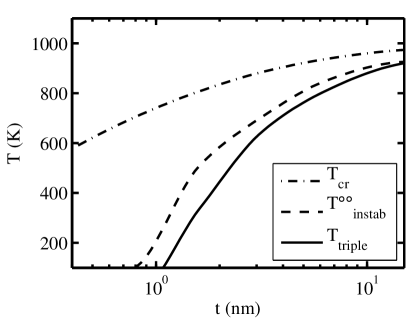
Figure 18: The temperatures of the critical points $T_{cr}$, the polar phase instabilities at $p_{O_{2}}=p^{\circ\circ}_{O_{2}}$, and the triple point, as a function of film thickness.

Figure 18 shows the temperatures as a function of film thickness of the critical points, the polar phase instabilities at $p_{O_{2}}/p^{\circ\circ}_{O_{2}}=1$, and the triple point. The triple point is the minimum equilibrium $T_{C}$. At temperatures between the triple point and the critical points, the nonpolar phase intervenes between the polar phases at equilibrium. An expression for the temperatures $T_{cr}$ of the critical points can be obtained by setting the second and third derivatives of the free energy simultaneously to zero, Eq. (36) and

$$0=\frac{\partial^{3}{\cal G}}{\partial\sigma^{3}}\approx tf^{\prime\prime\prime}(\sigma)-\frac{kT\left(1-\frac{2A_{i}\sigma}{z_{i}e}\right)}{z_{i}e\sigma^{2}\left(1-\frac{A_{i}\sigma}{z_{i}e}\right)^{2}},$$ (37)

where $i=\ominus$ or $\oplus$ as in Eq. (IV.2). In the approximation that $\sigma$ is small at the critical point, these reduce to

$$0\approx\approx\left(\alpha_{3}^{*}(T_{cr})+\frac{\lambda^{\dagger}}{\epsilon_{0}t}\right)^{3}+2\alpha_{33}^{*}\left(\frac{9kT_{cr}}{4t|z_{i}|e}\right)^{2}.$$ (38)

We use the double $\approx\approx$ symbol to indicate a rough approximation, in this case because it becomes invalid at small $t$. Nonetheless, Eq. (38) shows that the temperatures of the critical points for the ionic compensation case are suppressed by an additional thickness-dependent term not present in the electronic compensation case, Eq. (13). Even if the effective screening length is zero, $\lambda^{\dagger}=0$, the $T_{cr}$ are changed by an amount

$$\Delta T_{cr}\equiv T_{cr}-T_{C}^{\circ}\approx\approx-2\epsilon_{0}C(2\alpha_{33}^{*})^{1/3}\left(\frac{9kT_{cr}}{4t|z_{i}|e}\right)^{2/3}.$$ (39)

Using the LGD parametersGBS06JAP for PbTiO₃ coherently strained to SrTiO₃, $|z_{i}|=2$, and a thickness of $t=3.2$ nm, one obtains $\Delta T_{cr}\approx\approx-115$ K.

Figure 19 shows the internal field (along with the phase boundaries) as a function of $p_{O_{2}}/p^{\circ\circ}_{O_{2}}$ and $T$ for a 1.6 nm thick film. Like the electronic compensation cases, Figs. 6 and 10, the internal electric field is inverted in the polar phases near the phase boundaries because of the incompletely neutralized depolarizing field. While the electronic compensation model requires a nonzero screening length $\lambda$ to produce an inverted field, the ionic compensation model does not. The magnitude of the inverted field at the phase boundary is much larger for ionic than for electronic compensation in the cases shown. In all cases the inverted field regions extend above the critical point(s). The oxygen partial pressure corresponding to zero internal field can be obtained by setting the numerator in Eq. (28) to zero, giving

$$\ln p_{O_{2}}^{E_{in}=0} \approx -\frac{2n_{i}z_{i}e\lambda^{\dagger}P_{0}}{\epsilon_{0}kT}+n_{i}\ln\left(\frac{-A_{i}P_{0}/z_{i}e}{1+A_{i}P_{0}/z_{i}e}\right)$$ (40)

$$+ \frac{n_{i}\Delta G_{i}^{\circ\circ}}{kT},$$

where $P_{0}$ is the $T$-dependent zero-field spontaneous polarization of the epitaxially strained film given by the solution to Eq. (2) with $E_{in}=0$, and $i=\ominus$ or $\oplus$ for positive or negative values of $P_{0}$. As for electronic compensation, the conditions for zero field are independent of film thickness, and they intersect at $T_{C}^{\circ}$. Rough values of the oxygen partial pressure at the critical points $p_{O_{2}}^{cr}$ can be obtained by assuming that the field is zero and neglecting the first two terms in Eq. (40). This gives $kT_{cr}\ln p_{O_{2}}^{cr}\approx\approx n_{i}\Delta G_{i}^{\circ\circ}$, where $i=\ominus$ for positive $P$ (high $p_{O_{2}}$) and $i=\oplus$ for negative $P$ (low $p_{O_{2}}$).

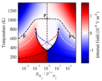
Figure 19: (Color online) Internal field for $t=1.6$ nm, corresponding to Fig. 17(b). Color scale gives electric field in stable phase. Dashed black curves show conditions for zero field, which intersect at $T_{C}^{\circ}$.

IV.4 Phase diagram for controlled surface oxygen density

It is instructive to plot equilibrium phase diagrams for ionic compensation as a function of the net excess surface oxygen density, defined by

$$\rho_{O}\equiv\sum_{i}\frac{2\theta_{i}}{n_{i}A_{i}}.$$ (41)

In the typical case where we can neglect one or the other of the $\theta_{i}$ for positive or negative $\sigma$, one obtains $\rho_{O}\approx 2\sigma/n_{i}z_{i}e$, for $i=\ominus$ or $\oplus$, so that $\rho_{O}$ is simply proportional to $\sigma$ for each range. Figures 20 and 21 show the polarization and internal field plotted as a color scale on $\rho_{O}$ vs. $T$ axes for $t=1.6$ nm. These correspond to the $p_{O_{2}}$ vs. $T$ diagrams shown in Figs. 17(b) and 19. Such controlled $\rho_{O}$ diagrams can be obtained using the Helmholtz free energy

$${\cal A} ={\cal G}+\frac{\rho_{O}}{2}kT\ln p_{O_{2}}\approx tf(\sigma)+\frac{\lambda^{\dagger}\sigma^{2}}{\epsilon_{0}}+\frac{\sigma\Delta G_{i}^{\circ\circ}}{z_{i}e}$$

$$+ \frac{kT}{A_{i}}\left[\frac{A_{i}\sigma}{z_{i}e}\ln\left(\frac{A_{i}\sigma}{z_{i}e}\right)+\left(1-\frac{A_{i}\sigma}{z_{i}e}\right)\ln\left(1-\frac{A_{i}\sigma}{z_{i}e}\right)\right],$$

where $i=\ominus$ or $\oplus$ as in Eq. IV.2.

Because $\rho_{O}$ is a conserved order parameter, the phase boundaries occuring on the controlled potential diagrams become two-phase fields on Figs. 20 and 21, as in the electronic compensation case for controlled surface charge, Figs. 9 and 10. These show the phase separation that would occur in a closed system if the net amount of excess surface oxygen is fixed, rather than the external $p_{O_{2}}$. The phase diagram for ionic compensation is more complex than that for electronic compensation; there are two equilibrium two-phase fields between polar and nonpolar phases above a tie-line at the triple point temperature.

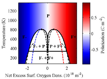
Figure 20: (Color online) Phase diagram as a function of net excess surface oxygen density $\rho_{O}$ and $T$ for 1.6 nm of PbTiO₃ coherently strained to SrTiO₃, corresponding to Fig. 17(b). Color scale gives polarization in single-phase region; three two-phase regions are marked. Solid and dash-dot black curves are stable and metastable phase boundaries, respectively, between nonpolar paraelectric (P) and positive and negative polar ferroelectric (F+ and F-) phases. Dashed red, blue, and black curves are metastability limits of the F+, F-, and P phases, respectively.

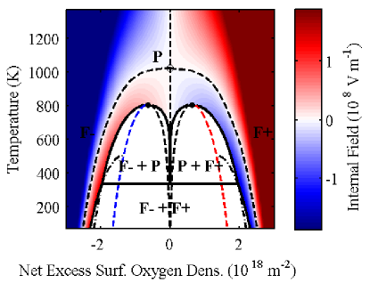
Figure 21: (Color online) Internal field corresponding to Fig. 20. Color scale gives electric field in stable phase. Dashed black curves show conditions for zero field, which intersect at $T_{C}^{\circ}$ (open circle).

V Discussion

The new parameters in the model developed above for ionic surface compensation are $n_{i}$, $z_{i}$, $A_{i}$, and $\Delta G_{i}^{\circ\circ}$ for $i=\ominus$ and $\oplus$, as well as $\lambda^{\prime}$. These can be related to the locations of the features on the phase diagram. Approximate expressions are given above that show how the $\Delta G_{i}^{\circ\circ}$ determine $p^{\circ\circ}_{O_{2}}$ and the $p_{O_{2}}^{cr}$, which give the center and width of the phase diagram in $p_{O_{2}}$ coordinates. These expressions are particularly simple when the phase diagram is symmetric in coordinates of $p_{O_{2}}/p^{\circ\circ}_{O_{2}}$ versus $T$, i.e. when $n_{\oplus}=-n_{\ominus}$, $z_{\ominus}=-z_{\oplus}$, and $A_{\ominus}=A_{\oplus}$. In this case one obtains $\ln p^{\circ\circ}_{O_{2}}=n_{\ominus}(\Delta G_{\ominus}^{\circ\circ}-\Delta G_{\oplus}^{\circ\circ})/(2kT)$, $\ln(p_{O_{2}}^{cr}/p^{\circ\circ}_{O_{2}})\approx\approx\pm n_{\ominus}(\Delta G_{\ominus}^{\circ\circ}+\Delta G_{\oplus}^{\circ\circ})/(2kT_{cr})$. The value of $\lambda^{\prime}$ affects the critical temperatures $T_{cr}$, which may be suppressed or enhanced relative to the electronic compensation value.

Although the phase diagrams we have shown are symmetric when plotted in $p_{O_{2}}/p^{\circ\circ}_{O_{2}}$ versus $T$ coordinates, the value of $p^{\circ\circ}_{O_{2}}$ is expected to be a function of $T$. Thus experimental phase diagrams obtained as a function of $p_{O_{2}}$ versus $T$ are not expected to be symmetric. Figure 22 shows the trajectories of constant $p_{O_{2}}$ on the same $T$ vs. $p_{O_{2}}/p^{\circ\circ}_{O_{2}}$ axes used to plot the phase diagrams. Note that we have neglected any temperature dependence of $\Delta G_{i}^{\circ\circ}$ in these calculations. Such temperature dependence might be expected since the entropy of O₂ in the environment may be different than that of the adsorbed ions.

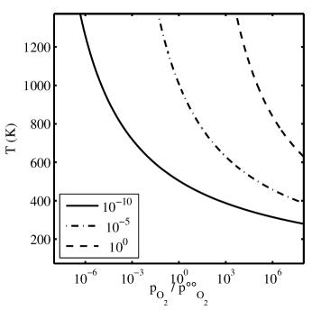
Figure 22: Curves show fixed values of $p_{O_{2}}$ (bar) given in the legend, plotted using same normalized axes used for the phase diagrams, with parameters corresponding to Table 2.

While the Gibbs free energy expressions for the ionic and electronic compensation cases are very similar, the phase diagrams differ qualitatively because a different parameter is fixed. If we neglect the polarization dependence of the $\Delta G_{i}^{\circ}$ so that $\lambda^{\prime}=0$ and we consider $\theta_{i}<<1$ for both $i=\ominus$ and $\oplus$, then by using the mass action equilibria Eqs. (22) one can show that the Gibbs free energy for ionic compensation, Eq. (30), reduces to Eq. (9) used for the fixed $V_{ex}$ case. However, the fixed $V_{ex}$ and fixed $p_{O_{2}}$ conditions lead to different equilibrium free energy surfaces, Figs. 3 and 14, even in the case of $\lambda^{\prime}=0$ and $\theta_{i}<<1$. The relationship between the fixed $V_{ex}$ and fixed $p_{O_{2}}$ conditions can be seen from Eq. (27). Here $p_{O_{2}}$ enters into the expression for $V_{ex}$ simply through the term $kT\ln p_{O_{2}}/(z_{i}n_{i}e)$. In general, however, fixed $p_{O_{2}}$ does not correspond to fixed $V_{ex}$ because there are other terms and they depend upon polarization. In particular, if the value of $\Delta G_{i}^{\circ\circ}/(z_{i}e)$ differs for positive and negative surface ions, then there is an abrupt jump in $V_{ex}$ when crossing $P=0$. Thus fixed $V_{ex}$ and fixed $p_{O_{2}}$ constraints produce different equilibrium behavior even when the free energy expression for both cases is the same.

The form of the phase diagrams in Fig. 17 in which a stable nonpolar phase intervenes between the polar phases is due to the appearance of a third local minimum in ${\cal G}(\sigma)$ near $\sigma=0$ as shown in Fig. 15. This is conceptually similar to the behavior of a ferroelectric with a first-order transition, for which the coefficient of $P^{4}$ in the free energy expression is negative. Strukov98 ; MERZ53PR For example, Figs. 23 and 24 in Appendix A show the phase diagrams for controlled internal field $E_{in}$ and net surface charge $\bar{\sigma}$ for unstressed bulk PbTiO₃ with ideal electrodes ($\lambda=0$). Here the topology of the equilibrium phase boundaries is similar to that in Figs. 17(a,b) and 20, with a triple point and two critical points. However, the range of temperatures spanned by this structure in ultrathin films with ionic compensation can be much larger than in bulk PbTiO₃. Furthermore, the polarization of the paraelectric phase at temperatures below the critical points is much closer to zero in ultrathin films with ionic compensation, because of the sharp minimum in ${\cal G}(\sigma)$ at $\sigma=0$.

The appearance of a stable nonpolar state between the polar states on the $p_{O_{2}}$ vs. $T$ phase diagram can affect the mechanism of switching and the internal field at which switching occurs (i.e. the coercive field). During switching by ramping $p_{O_{2}}$, the film may first become unstable with respect to the nonpolar state before reaching $p_{O_{2}}$ values that stabilize the opposite polarization, thus suppressing nucleation of oppositely polarized domains. In this case the internal field could reach the intrinsic coercive field and switching occur by a continuous, spinodal mechanism without nucleation. This could produce the recently observed crossover to a continuous mechanism10_HighlandPRL through an equilibrium pathway not requiring kinetic suppression of nucleation.

The model developed here contains several assumptions that could be relaxed in future extensions. We assume that the effective screening length $\lambda$ is not negative, so that electronic interfacial effects tend to suppress rather than enhance polarization in ultrathin films. We also neglect any polarization dependence of $\lambda$. Ab initio calculations09_Stengel_NatMat ; 09_StengelPRB_80_224110 indicate that in some systems the interfaces enhance film polarization, which can be modeled with a negative $\lambda$, and that $\lambda$ depends on $P$. These effects could be included by modifications to our electrostatic boundary conditions and free energy expressions. We constrain the free and bound charge at each interface to reside in single planes, so that there is no space charge. Such space charge could be included as has been done previously in models with semiconducting ferroelectric films and/or electrodes.BAT73PRL ; BAT73JVST ; WURF76FERRO ; BRAT00PRB Since the screening layer of thickness $\lambda$ is a conceptual construct rather than an actual dielectric layer in our model, we do not consider tunneling of free charge across this layer, which has been recently considered for systems with a dielectric separating the electrode from the ferroelectric.JIANG09PRB These effects could be added for such systems. We also neglect the possibility of equilibrium 180^∘ stripe domain formation02_StriefferPRL_89_067601 ; 04_Fong_Science ; GBS06JAP ; LAI07APL ; CT08APL ; BRAT08JCTN in which nanoscale domain structures reduce the depolarizing field even when there is little or no electronic or ionic compensation charge at one or both interfaces. A full treatment of equilibrium stripe domains for the ionic compensation case would be valuable in future work.

VI Summary and Conclusions

Ionic compensation of a ferroelectric surface due to chemical equilibrium with an environment introduces new features into the phase diagrams, Figs. 17 and 20, not present in the standard phase diagrams for a second-order transition in a film with electronic compensation, Figs. 5 and 9. The constant $p_{O_{2}}$ chemical boundary condition shown in Fig. 13 is a hybrid between the constant $V_{ex}$ and constant $\sigma$ boundary conditions shown in Fig. 2. Because the surface concentrations of ionic species $\theta_{i}$ are limited to values between zero and unity, constant surface charge regimes occur when the $\theta_{i}$ are saturated. In the regimes where one of the $\theta_{i}$ is varying between these limits, the boundary condition is similar to a fixed $V_{ex}$ condition. There are two independent relations for the surface charge $\sigma$ as a function of $p_{O_{2}}$, depending upon whether positive or negative surface ions predominate. In the $p_{O_{2}}$ region where there is insufficient surface charge of either sign to stabilize a polar state, the nonpolar state becomes stable between the positive and negative polar states, producing two critical points, a triple point, and a strong dependence of $T_{C}$ on $p_{O_{2}}$. Large inverted internal fields occur at equilibrium in the polar phases near the phase boundaries with the nonpolar phase. Manipulation of ultrathin ferroelectric films via controlled ionic compensation may thus allow experimental access to exotic nonpolar and high-field states such as those modeled in recent ab initio calculations09_StengelNatPhys_5_304 ; BECKMAN09PRB that would not be stable under electronic compensation conditions.

Appendix A Phase Diagrams for First-Order Ferroelectric

The phase diagrams for a bulk ferroelectric that has a first-order transition at zero field are similar to those for ultrathin films with ionic surface compensation. Here we present calculated phase diagrams showing the region near the critical points for the weakly first-order transition in unstressed bulk PbTiO₃. The features in these phase diagrams can be compared with those for ultrathin epitaxially strained films shown above, which have a second-order transition for electronic compensation but a strongly first-order transition for ionic surface compensation.

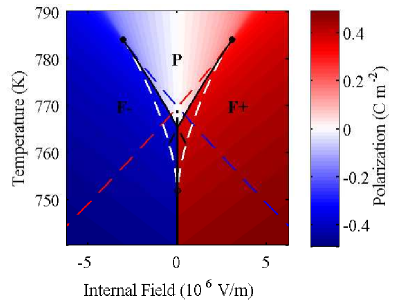
Figure 23: (Color online) Region near critical points on equilibrium polarization phase diagram as a function of $E_{in}$ and $T$, for unstressed bulk PbTiO₃ with ideal electrodes ($\lambda=0$). Color scale gives polarization of stable phase. Solid and dash-dot black curves are stable and metastable phase boundaries, respectively, between nonpolar paraelectric (P) and positive and negative polar ferroelectric (F+ and F-) phases. Dashed red, blue, and white curves are metastability limits of the F+, F-, and P phases, respectively.

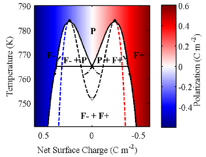
Figure 24: (Color online) Region near critical points on equilibrium polarization phase diagram for unstressed bulk PbTiO₃ with ideal electrodes ($\lambda=0$) corresponding to Fig. 23, here plotted as a function of net surface charge ${\bar{\sigma}}$ and $T$. Color scale gives polarization in single-phase region, which is separated by phase boundary (solid black curve) from three two-phase fields; metastable phase boundaries are dash-dot curves, and two critical points are marked by filled circles. Dashed red, blue, and black curves are metastability limits of the F+, F-, and P phases, respectively.

These phase diagrams are calculated using the Landau-Ginzburg-Devonshire expression for the free energy per unit volume of unstressed bulk PbTiO₃ with ideal electrodes having zero screening length ($\lambda=0$),

$${\cal G}_{v}=\alpha_{1}P^{2}+\alpha_{11}P^{4}+\alpha_{111}P^{6}+\epsilon_{0}E_{in}^{2}/2-E_{in}P$$ (43)

with $\alpha_{1}=(T-T_{0})/2\epsilon_{0}C$, where the parameters are given in Table I of the main paper. Figure 23 shows the phase diagram for controlled internal field $E_{in}$ and Fig. 24 shows the phase diagram for controlled net surface charge $\bar{\sigma}$. These are typical for a ferroelectric with a first-order transition, for which the coefficient of $P^{4}$ in the free energy expression is negative. The topology of the equilibrium phase boundaries is similar to the ionic compensation case, Figs. 17(a,b) and 20, with a triple point and two critical points. However, the paraelectric phase above the triple point has a much wider range of polarization around zero in this case, reflecting the relatively broad minimum in ${\cal G}_{v}$ near $P=0$.

References

- (1) S. K. Streiffer et al., Phys. Rev. Lett. 89, 067601 (2002).
- (2) D. D. Fong et al., Science 304, 1650 (2004).
- (3) G. B. Stephenson and K. R. Elder, J. Appl. Phys. 100, 051601 (2006).
- (4) B.-K. Lai, I. Ponomareva, I. Kornev, L. Bellaiche, and G. Salamo, Appl. Phys. Lett. 91, 152909 (2007).
- (5) C. Thompson et al., Appl. Phys. Lett. 93, 182901 (2008).
- (6) A. M. Bratkovsky and A. P. Levanyuk, J. Computat. Theor. Nanoscience 6, 465 (2009).
- (7) I. P. Batra, P. Wurfel, and B. D. Silverman, Phys. Rev. Lett. 30, 384 (1973).
- (8) I. P. Batra, P. Wurfel, and B. D. Silverman, J. Vac. Sci. Technol. 10, 687 (1973).
- (9) P. Wurfel and I. P. Batra, Ferroelectrics 12, 55 (1976).
- (10) M. Dawber, P. Chandra, P. B. Littlewood, and J. F. Scott, J. Phys.: Condens. Matter 15, L393 (2003).
- (11) A. K. Tagantsev and G. Gerra, J. Appl. Phys. 100, 051607 (2006).
- (12) J. Junquera and P. Ghosez, Nature 422, 506 (2003).
- (13) N. Sai, A. M. Kolpak, and A. M. Rappe, Phys. Rev. B 72, 020101(R) (2005).
- (14) M. Stengel, D. Vanderbilt, and N. A. Spaldin, Nature Materials 8, 392 (2009).
- (15) C. Lichtensteiger, J.-M. Triscone, J. Junquera, and P. Ghosez, Phys. Rev. Lett. 94, 047603 (2005).
- (16) D. D. Fong et al., Phys. Rev. Lett. 96, 127601 (2006).
- (17) L. Despont et al., Phys. Rev. B 73, 094110 (2006).
- (18) C. Lichtensteiger et al., Appl. Phys. Lett. 90, 052907 (2007).
- (19) S. V. Kalinin and D. A. Bonnell, Nano Lett. 4, 555 (2004).
- (20) R.-V. Wang et al., Phys. Rev. Lett. 102, 047601 (2009).
- (21) Y. Kim, I. Vrejoiu, D. Hesse, and M. Alexe, Appl. Phys. Lett. 96, 202902 (2010).
- (22) M. J. Highland et al., Phys. Rev. Lett. 105, 167601 (2010).
- (23) M. Dawber, K. M. Rabe, and J. F. Scott, Rev. Mod. Phys. 77, 1083 (2005).
- (24) J. E. Spanier et al., Nano Lett. 6, 735 (2006).
- (25) J. Shin et al., Nano Lett. 9, 3720 (2009).
- (26) W. Schmickler, Interfacial Electrochemistry (Oxford Univ. Press, Oxford, 1996), chap. 4.
- (27) R. Kretschmer and K. Binder, Phys. Rev. B 20, 1065 (1979).
- (28) V. G. Koukhar, N. A. Pertsev, and R. Waser, Phys. Rev. B 64, 214103 (2001).
- (29) M. Stengel and N. A. Spaldin, Nature 443, 679 (2006).
- (30) M. Stengel, D. Vanderbilt, and N. A. Spaldin, Phys. Rev. B 80, 224110 (2009).
- (31) N. A. Pertsev, A. G. Zembilgotov, and A. K. Tagantsev, Phys. Rev. Lett. 80, 1988 (1998).
- (32) M. J. Haun, E. Furman, S. J. Jang, H. A. McKinstry, and L. E. Cross, J. Appl. Phys. 62, 3331 (1987).
- (33) G. A. Rossetti, Jr., J. P. Cline, and A. Navrotsky, J. Mater. Res. 13, 3197 (1998).
- (34) M. Stengel, N. A. Spaldin, and D. Vanderbilt, Nature Physics 5, 304 (2009).
- (35) J. W. Cahn and J. E. Hilliard, J. Chem. Phys. 31, 688 (1959).
- (36) B. A. Strukov and A. P. Levanyuk, Ferroelectric Phenomena in Crystals (Springer, Berlin, 1998) p. 69.
- (37) S. Salahuddin and S. Datta, Nano Lett. 8, 405 (2008).
- (38) A. Artemev and A. Roytburd, Acta Mater. 58, 1004 (2010).
- (39) W. J. Merz, Phys. Rev. 91, 513 (1953).
- (40) A. M. Bratkovsky and A. P. Levanyuk, Phys. Rev. B 61, 15042 (2000).
- (41) A.-Q. Jiang, H. J. Lee, C. S. Hwang, and T.-A. Tang, Phys. Rev. B 80, 024119 (2009).
- (42) S. P. Beckman, X. Wang, K. M. Rabe, and D. Vanderbilt, Phys. Rev. B 79, 144124 (2009).