A Graphical Approach to a Model of Neuronal Tree with Variable Diameter

Abstract.

We propose a simple graphical approach to steady state solutions of the cable equation for a general model of dendritic tree with tapering. A simple case of transient solutions is also briefly discussed.

1. Introduction

The function of many physiological systems depends on branched structures that exist both at the tissue (e.g. nervous plexi, lungs, and the vascular and lymphatic systems) and the cellular level (e.g. neurons). Of particular interest, local and global propagation of electrical signals within the nervous system depends on the integration, processing, and further generation of electrical pulses that travel through neurons. In turn, the tree-like morphology of neurons facilitates simultaneous signaling to cells located in different places and over long distances.

Neuronal morphology is typically modeled by assuming that the shape of small neuronal segments, or neurites, is approximated by cylinders of different diameters. As a consequence, cable theory [45], [46], [47], [48], [49], [50] plays a central role in the theoretical and experimental study of electrical conduction in neurons; see, for example [8], [11], [59], [14], [19], [20], [21], [22], [23], [31], [53], [57] and references therein. Notably, one of the most interesting results from recent theoretical work is that geometrical properties of neuronal membranes may exert powerful effects on signal propagation even in the presence of voltage-dependent channels [60].

Theoretical research involving realistic neuronal morphologies is typically done by numerically solving systems of cable equations defined on cylinders with different radii, and assuming that voltage and current are continuous functions of space and time. To the best of our knowledge, graphical methods seem have not been widely applied yet in the mathematical modeling of neurons. Graphical methods are very useful and popular in different branches of modern physics. It is worth noting, for example, Feynman diagrams in quantum mechanical or statistical field theory [3], [4], [10], [25], [26], [27], [32], [37], [63], Vilenkin-Kuznetsov-Smorodinskii approach to solutions of $n$-dimensional Laplace equation [38], [42], [54], [55], applications in solid-state theory, etc. A goal of this paper is to make a modest step in this direction (see also [1], [14] and references therein). We use explicit solutions from recent papers on variable quadratic Hamiltonians in nonrelativistic quantum mechanics [12], [15], [16], [17], [18], [35], [38], [56], [58] to describe steady state and transient solutions to linear cable equations modeling neurites with non-necessarily constant radius.

2. Cable Equation with Varying Radius

At a closer view, neurites can be regarded as volumes of revolution, defined by rotating a smooth function $r=r(x)$ representing the local radius of the neurite where $x$ represents distance along the neurite. As a result, the cable theory implies the following set of equations [31], [47]:

$$2\pi rI_{m}\frac{ds}{dx}=-\frac{\partial I}{\partial x},\qquad\frac{ds}{dx}=\sqrt{1+\left(\frac{dr}{dx}\right)^{2}}$$ (2.1)

$$I_{m}=\frac{V}{R_{m}}+C_{m}\frac{\partial V}{\partial t},$$ (2.2)

$$I=-\frac{\pi r^{2}}{R_{i}}\frac{\partial V}{\partial x}.$$ (2.3)

Here, $V$ represents the voltage difference across the membrane (interior minus exterior) as a deviation from its resting value, $I_{m}$ is the membrane current density, $I=I_{a}$ is the total axial current, $R_{m}$ is the membrane resistance, $R_{i}$ is the intercellular resistivity and $C_{m}$ is membrane capacitance (more details can be found in [31], [45] and [47]). Differentiating equation (2.3) with respect to $x$ and substituting the result into (2.1) with the help of (2.2) one gets

$$\left(V+C_{m}R_{m}\frac{\partial V}{\partial t}\right)\sqrt{1+\left(\frac{dr}{dx}\right)^{2}}=\frac{R_{m}}{2R_{i}}\frac{1}{r}\frac{\partial}{\partial x}\left(r^{2}\frac{\partial V}{\partial x}\right),$$ (2.4)

which is the cable equation with tapering for a single branch of dendritic tree (see [19], [31], [47] and [57] for more details).

We shall be particularly interested in solutions of the cable equation (2.4) corresponding to termination with a “sealed end”, namely, when at the end point $x=x_{1}$ the membrane cylinder is sealed with a disk composed of the same membrane. In this case, the corresponding boundary condition can be derived by setting

$$I_{a}=\pi r^{2}I_{m},$$ (2.5)

at $x=x_{1}.$ Then, in view of (2.2)–(2.3), one gets [45]:

$$\left.\left(V+C_{m}R_{m}\frac{\partial V}{\partial t}+\frac{R_{m}}{R_{i}}\frac{\partial V}{\partial x}\right)\right|_{x=x_{1}}=0,\qquad t\geq 0.$$ (2.6)

In a similar fashion, at the somatic end one gets

$$\left.\left(V+C_{s}R_{s}\frac{\partial V}{\partial t}-\frac{R_{s}}{R_{i}}\frac{\partial V}{\partial x}\right)\right|_{x=x_{0}}=0,\qquad t\geq 0,$$ (2.7)

where $R_{s}$ is the somatic resistance and $C_{s}$ is the somatic capacitance [20]. We shall use these conditions for the steady-state and transient solutions of the cable equation. (Later we may impose similar boundary conditions at the points of branching.)

In this Letter, we shall first concentrate on steady-state solutions of the cable equation, when $\partial V/\partial t\equiv 0.$ Then

$$V\sqrt{1+\left(\frac{dr}{dx}\right)^{2}}=\frac{R_{m}}{2rR_{i}}\frac{d}{dx}\left(r^{2}\frac{dV}{dx}\right)\qquad\left(x_{0}\leq x\leq x_{1}\right)$$ (2.8)

and

$$\left.V\right|_{x=x_{0}}=V_{0},\qquad\left.\left(\frac{dV}{dx}+B\left(x\right)V\right)\right|_{x=x_{1}}=0,\qquad B\left(x_{1}\right)=\frac{R_{i}}{R_{m}}.$$ (2.9)

This boundary value problem can be conveniently solved (by a direct substitution for each branch of the dendritic tree) in terms of standard solutions of this second order ordinary differential equation as follows

$$V\left(x\right)=V\left(x_{0}\right)\frac{C\left(x\right)+B\left(x_{1}\right)S\left(x\right)}{C\left(x_{0}\right)+B\left(x_{1}\right)S\left(x_{0}\right)},$$ (2.10)

where $C\left(x\right)$ and $S\left(x\right)$ are two linearly independent solutions of the stationary cable equation (2.8) that satisfy special boundary conditions $C\left(x_{1}\right)=1,$ $C^{\prime}\left(x_{1}\right)=0$ and $S\left(x_{1}\right)=0,$ $S^{\prime}\left(x_{1}\right)=-1.$ Then

$$\frac{dV}{dx}+B\left(x\right)V=0\qquad\left(x_{0}\leq x\leq x_{1}\right)$$ (2.11)

with the corresponding current density/voltage ratio function $B\left(x\right)$ given by

$$B\left(x\right)=-\frac{V^{\prime}}{V}=-\frac{C^{\prime}\left(x\right)+B\left(x_{1}\right)S^{\prime}\left(x\right)}{C\left(x\right)+B\left(x_{1}\right)S\left(x\right)}$$ (2.12)

in term of the standard solutions $C\left(x\right)$ and $S\left(x\right).$ Throughout this Letter, we shall refer to a case, when $B\left(x\right)>0\ \left(x_{0}<x<x_{1}\right),$ as the case of weak tapering. An opposite situation, when $B\left(\xi\right)=0$ at certain point $x_{0}<\xi<x_{1}$ and an inverse of the current may occur, shall be called a case of the strong tapering. (A case of strong tapering has been numerically discovered in [28].)

3. Tapering with Analytic, Asymptotic and/or Numerical Solutions

In this Letter, we consider a general model of a dendrite as a (binary) directed tree (from the soma to its terminal ends) consisting of axially symmetric branches with the following types of tapering.

3.1. Cylinder

Here, $r=r_{0}=$constant, $0\leq x\leq L$ and the cable equation takes the simplest form

$$\lambda^{2}\frac{d^{2}V}{dx^{2}}=V,\qquad\lambda^{2}=\frac{r_{0}R_{m}}{2R_{i}}$$ (3.1)

with a familiar solution [31], [45], [47]:

$$V\left(x\right)=V_{0}\frac{\cosh\left(\left(L-x\right)/\lambda\right)+\lambda B_{L}\sinh\left(\left(L-x\right)/\lambda\right)}{\cosh\left(L/\lambda\right)+\lambda B_{L}\sinh\left(L/\lambda\right)}$$ (3.2)

subject to boundary conditions

$$V\left(0\right)=V_{0},\qquad B_{L}V\left(L\right)+\frac{dV}{dx}\left(L\right)=0.$$ (3.3)

Then

$$B\left(x\right)=\frac{\lambda B_{L}+\tanh\left(\left(L-x\right)/\lambda\right)}{\lambda+\lambda^{2}B_{L}\tanh\left(\left(L-x\right)/\lambda\right)}.$$ (3.4)

(See [31], [47], [49], [50], [59] and references therein for more details.)

3.2. Frustum(Cone)

Here, $r=r\left(x\right)=r_{0}+\frac{r_{1}-r_{0}}{L}x$ with $0\leq x\leq L.$ The steady-state solution of the corresponding cable equation

$$r\frac{d^{2}V}{dx^{2}}+2\frac{dV}{dx}=\frac{\mu^{2}}{4}V,\qquad\mu=\sqrt{\frac{8R_{i}}{R_{m}}}\frac{\left(1+\left(\frac{r_{1}-r_{0}}{L}\right)^{2}\right)^{1/4}}{\left|\frac{r_{1}-r_{0}}{L}\right|}$$ (3.5)

subject to boundary conditions (3.3) are given by [7]

$$V\left(x\right)=V_{0}\frac{C\left(L-x\right)+B_{L}S\left(L-x\right)}{C\left(L\right)+B_{L}S\left(L\right)}.$$ (3.6)

Here, the standard solutions that satisfy $S\left(0\right)=0,$ $S^{\prime}\left(0\right)=1$ and $C\left(0\right)=1,$ $C^{\prime}\left(0\right)=0$ can be constructed as follows

$$S\left(x\right)=\frac{2Lr_{0}^{3/2}}{\left(r_{1}-r_{0}\right)\sqrt{r}}\left[K_{1}\left(\mu\sqrt{r_{0}}\right)I_{1}\left(\mu\sqrt{r}\right)-I_{1}\left(\mu\sqrt{r_{0}}\right)K_{1}\left(\mu\sqrt{r}\right)\right]$$ (3.7)

and

$$C\left(x\right) = \left[\mu\sqrt{r_{0}}K_{0}\left(\mu\sqrt{r_{0}}\right)+2K_{1}\left(\mu\sqrt{r_{0}}\right)\right]\sqrt{\frac{r_{0}}{r_{1}}}I_{1}\left(\mu\sqrt{r}\right)$$

$$+\left[\mu\sqrt{r_{0}}I_{0}\left(\mu\sqrt{r_{0}}\right)-2I_{1}\left(\mu\sqrt{r_{0}}\right)\right]\sqrt{\frac{r_{0}}{r_{1}}}K_{1}\left(\mu\sqrt{r}\right)$$

in terms of modified Bessel functions $I_{\nu}\left(z\right)$ and $K_{\nu}\left(z\right)$ of orders $\nu=0,1$ (different aspects of the advanced theory of Bessel functions can be found in [2], [5], [6], [24], [41], [43], [44], [61] and [62]).

3.3. Hyperbola

If $r=a\cosh\left(\frac{x-b}{a}\right)$ on an interval $x_{0}\leq x\leq x_{1},$ the cable equation (2.4) takes the form

$$\left(V+C_{m}R_{m}\frac{\partial V}{\partial t}\right)\cosh\left(\frac{x-b}{a}\right)=\frac{R_{m}}{2R_{i}}\left[2\sinh\left(\frac{x-b}{a}\right)\frac{\partial V}{\partial x}+a\cosh\left(\frac{x-b}{a}\right)\frac{\partial^{2}V}{\partial x^{2}}\right].$$ (3.9)

This special case of tapering is integrable in terms of elementary functions [30] (see also [12] and [17] for a similar problem related to a model of the dumped quantum oscillator). For the steady-state solutions one obtains the following equation

$$V^{\prime\prime}+2\lambda\tanh\left(\lambda x+\delta\right)V^{\prime}=\mu_{0}^{2}V$$ (3.10)

with new parameters

$$\lambda=\frac{1}{a},\qquad\delta=-\lambda b,\qquad\mu_{0}^{2}=\frac{2R_{i}}{aR_{m}}.$$ (3.11)

The corresponding two linearly independent solutions, namely,

$$V_{1}\left(x\right)=\frac{\sinh\left(\mu x+\gamma\right)}{\cosh\left(\lambda x+\delta\right)},\qquad V_{2}\left(x\right)=\frac{\cosh\left(\mu x+\gamma\right)}{\cosh\left(\lambda x+\delta\right)},\qquad\mu=\sqrt{\mu_{0}^{2}+\lambda^{2}},$$ (3.12)

can be verified by a direct substitution for an arbitrary parameter $\gamma.$

The required steady-state solution of the boundary value problem

$$V\left(x_{0}\right)=V_{0},\qquad BV\left(x_{1}\right)+\frac{dV}{dx}\left(x_{1}\right)=0$$ (3.13)

is given by

$$V\left(x\right)=V_{0}\frac{C\left(x_{1}-x\right)+BS\left(x_{1}-x\right)}{C\left(x_{1}-x_{0}\right)+BS\left(x_{1}-x_{0}\right)},$$ (3.14)

where

$$C\left(x_{1}-x\right)=\cosh\left(\lambda\left(b-x_{1}\right)\right)\frac{\cosh\left(\mu\left(x_{1}-x\right)\right)}{\cosh\left(\lambda\left(x-b\right)\right)}$$ (3.15)

$$\quad\qquad\qquad\quad+\sinh\left(\lambda\left(b-x_{1}\right)\right)\frac{\lambda\sinh\left(\mu\left(x_{1}-x\right)\right)}{\mu\cosh\left(\lambda\left(x-b\right)\right)}$$

and

$$S\left(x_{1}-x\right)=\cosh\left(\lambda\left(b-x_{1}\right)\right)\frac{\sinh\left(\mu\left(x_{1}-x\right)\right)}{\mu\cosh\left(\lambda\left(x-b\right)\right)}.$$ (3.16)

(See [30] for more details.)

3.4. General Case of Axial Symmetry

One can use numerical methods and/or WKB-type approximation in order to obtain standard solutions. For example [41],

$$V\approx\frac{1}{\sqrt{r^{2}\left(x\right)p\left(x\right)}}\left[Ae^{\xi\left(x\right)}+Be^{-\xi\left(x\right)}\right],$$ (3.17)

where

$$p\left(x\right)=\left(\frac{2}{r}\frac{ds}{dx}\frac{R_{i}}{R_{m}}\right)^{1/2},\qquad\xi\left(x\right)=\int_{x_{0}}^{x}p\left(t\right)\ dt.$$ (3.18)

(See [31] and [47] for further details.)

4. A Graphical Approach

Graphical rules for steady-state voltages and currents in a model of dendritic tree with tapering are as follows.

4.1. Single Axially Symmetric Branch with Arbitrary Tapering

For a single branch with tapering voltage and current density/voltage ratio are given by

$$V\left(x\right) = \frac{C\left(x_{1}-x\right)+B\left(x_{1}\right)S\left(x_{1}-x\right)}{C\left(x_{1}-x_{0}\right)+B\left(x_{1}\right)S\left(x_{1}-x_{0}\right)}V\left(x_{0}\right)$$

$$= \left(C\left(x_{1}-x\right)+B\left(x_{1}\right)S\left(x_{1}-x\right)\right)V\left(x_{1}\right),$$

$$B\left(x\right)=\frac{C^{\prime}\left(x_{1}-x\right)+B\left(x_{1}\right)S^{\prime}\left(x_{1}-x\right)}{C\left(x_{1}-x\right)+B\left(x_{1}\right)S\left(x_{1}-x\right)}=-\frac{V^{\prime}\left(x\right)}{V\left(x\right)},$$ (4.2)

respectively (see Figure 1).

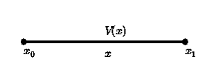
Figure 1. A Single Branch with Tapering.

4.2. Junction of Three Branches with Different Types of Tapering

The internal potential and current are assumed to be continuous at all dendritic branch points and at the soma-dendritic junction [45]. We consider a general case when each branch has its own tapering, say $r=r\left(x\right),$ $r_{1}=r_{1}\left(x\right)$ and $r_{2}=r_{2}\left(x\right)$ (see Figure 2). Then

$$V\left(x_{12}\right)=V_{1}\left(x_{12}\right)=V_{2}\left(x_{12}\right),$$ (4.3)

$$r^{2}\left(x_{12}\right)B\left(x_{12}\right)=r_{1}^{2}\left(x_{12}\right)B_{1}\left(x_{12}\right)+r_{2}^{2}\left(x_{12}\right)B_{2}\left(x_{12}\right).$$ (4.4)

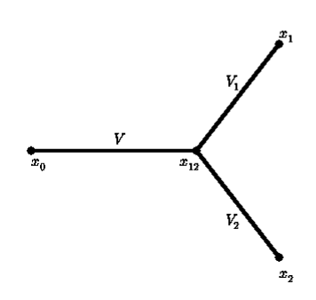
Figure 2. A Junction of Three Different Branches.

The total ratio constant $B\left(x_{12}\right)$ at the branching point $x_{12}$ is given by the following expression

$$B\left(x_{12}\right) = \frac{r_{1}^{2}\left(x_{12}\right)}{r^{2}\left(x_{12}\right)}B_{1}\left(x_{12}\right)+\frac{r_{2}^{2}\left(x_{12}\right)}{r^{2}\left(x_{12}\right)}B_{2}\left(x_{12}\right)$$

$$= B\left(B_{1}\left(x_{1}\right),B_{2}\left(x_{2}\right)\right)$$

$$= \frac{r_{1}^{2}\left(x_{12}\right)}{r^{2}\left(x_{12}\right)}\frac{C_{1}^{\prime}\left(x_{1}-x_{12}\right)+B_{1}\left(x_{1}\right)S_{1}^{\prime}\left(x_{1}-x_{12}\right)}{C_{1}\left(x_{1}-x_{12}\right)+B_{1}\left(x_{1}\right)S_{1}\left(x_{1}-x_{12}\right)}$$

$$+\frac{r_{2}^{2}\left(x_{12}\right)}{r^{2}\left(x_{12}\right)}\frac{C_{2}^{\prime}\left(x_{2}-x_{12}\right)+B_{2}\left(x_{2}\right)S_{2}^{\prime}\left(x_{2}-x_{12}\right)}{C_{2}\left(x_{2}-x_{12}\right)+B_{2}\left(x_{2}\right)S_{2}\left(x_{2}-x_{12}\right)}.$$

Then the ratio constant $B\left(x_{0}\right)$ is

$$B\left(x_{0}\right)=\frac{C^{\prime}\left(x_{12}-x_{0}\right)+B\left(x_{12}\right)S^{\prime}\left(x_{12}-x_{0}\right)}{C\left(x_{12}-x_{0}\right)+B\left(x_{12}\right)S\left(x_{12}-x_{0}\right)}$$ (4.6)

with the coefficient $B\left(x_{12}\right)$ found by the previous formula (4.2).

4.3. Junction of $\left(n+1\right)$-Branches

In a similar fashion, at the branching point $x_{\alpha},$ one gets

$$V\left(x_{\alpha}\right)=V_{1}\left(x_{\alpha}\right)=V_{2}\left(x_{\alpha}\right)=...=V_{n}\left(x_{\alpha}\right),$$ (4.7)

$$r^{2}\left(x_{\alpha}\right)B\left(x_{\alpha}\right) = r_{1}^{2}\left(x_{\alpha}\right)B_{1}\left(x_{\alpha}\right)+r_{2}^{2}\left(x_{\alpha}\right)B_{2}\left(x_{\alpha}\right)+...+r_{n}^{2}\left(x_{\alpha}\right)B_{n}\left(x_{\alpha}\right)$$

$$= \sum_{i=1}^{n}r_{i}^{2}\left(x_{\alpha}\right)B_{i}\left(x_{\alpha}\right).$$

(See Figure 3.)

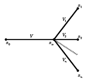
Figure 3. A Junction of $(n+1)$-Branches.

Combination of the above graphical rules results in a simple algorithm of evaluation of voltages and currents in the model of dendritic tree under consideration as follows.

Evaluate constants $B\left(x_{\alpha}\right)$ for all branching points of the tree: (a) first apply formula (4.2) for all open notes; (b) remove the above nodes from the tree and keep repeating the previous step until you reach the root of tree (soma).

In order to find voltage at a point $x$ of the dendritic tree, follow the path $x_{0}\rightarrow x$ and multiply the initial voltage $V\left(x_{0}\right)$ by consecutive corresponding factors from formula (4.1) changing at each intersection of the tree. The ratio of voltages $V\left(x_{\alpha}\right)$ and $V\left(x_{\beta}\right)$ at two terminal points, can be determine in a graphic form by the previous rule applied to the shortest path $x_{\beta}\rightarrow x_{\beta}.$

5. Examples

Our formulas (4.2)–(4.6) define ratio coefficients $B\left(x_{\alpha}\right)$ for all vertexes for the standard node on Figure 2. For the corresponding voltages, one can write

$$V\left(x_{0}\right) = \left[C\left(x_{12}-x_{0}\right)+B\left(x_{12}\right)S\left(x_{12}-x_{0}\right)\right]V\left(x_{12}\right)$$

$$= \left[C\left(x_{12}-x_{0}\right)+B\left(x_{12}\right)S\left(x_{12}-x_{0}\right)\right]V\left(x_{12}\right)$$

$$\times\left[C\left(x_{1}-x_{12}\right)+B\left(x_{1}\right)S\left(x_{1}-x_{12}\right)\right]V\left(x_{1}\right)$$

$$= \left[C\left(x_{12}-x_{0}\right)+B\left(x_{12}\right)S\left(x_{12}-x_{0}\right)\right]V\left(x_{12}\right)$$

$$\times\left[C\left(x_{2}-x_{12}\right)+B\left(x_{2}\right)S\left(x_{2}-x_{12}\right)\right]V\left(x_{2}\right)$$

and

$$\frac{V\left(x_{1}\right)}{V\left(x_{2}\right)}=\frac{C\left(x_{2}-x_{12}\right)+B\left(x_{2}\right)S\left(x_{2}-x_{12}\right)}{C\left(x_{1}-x_{12}\right)+B\left(x_{1}\right)S\left(x_{1}-x_{12}\right)}.$$ (5.2)

Further examples are left to the reader.

6. Transient Solutions

6.1. A Single Branch with Smooth Tapering

Let us consider the cable equation (2.4) for a single branch with an arbitrary smooth tapering $r=r\left(x\right)$ on the interval $x_{0}\leq x\leq x_{1}.$ The separation of variables

$$V\left(x,t\right)=e^{-\left(1+\alpha^{2}\right)t/\tau_{m}}U\left(x\right),\qquad\tau_{m}=C_{m}R_{m}$$ (6.1)

in results in

$$\frac{1}{r}\frac{d}{dx}\left(r^{2}\frac{dU}{dx}\right)+\omega^{2}\frac{ds}{dx}U=0,\qquad\omega^{2}=\frac{2R_{i}}{R_{m}}\alpha^{2},$$ (6.2)

where $\alpha$ is a separation constant. The boundary condition at the sealed end (2.6) takes the form

$$\left.\left(\frac{dU}{dx}-\frac{1}{2}\omega^{2}U\right)\right|_{x=x_{1}}=0.$$ (6.3)

A general solution of this problem can be conveniently written (for each branch of the dendritic tree) as follows

$$U\left(x\right)=U\left(x,\omega\right)=A\left[C\left(x,\omega\right)+\frac{1}{2}\omega^{2}S\left(x,\omega\right)\right],$$ (6.4)

where $A$ is a constant and $C\left(x,\omega\right)$ and $S\left(x,\omega\right)$ are two linearly independent standard solutions of equation (6.2) that satisfy special boundary conditions $C\left(x_{1},\omega\right)=1,$ $C^{\prime}\left(x_{1},\omega\right)=0$ and $S\left(x_{1},\omega\right)=0,$ $S^{\prime}\left(x_{1},\omega\right)=1.$ Then the boundary condition (2.7) at the somatic end $x=x_{0},$ namely,

$$\left.\left(\frac{dU}{dx}+\left[\frac{R_{i}}{R_{s}}\left(\frac{\tau_{s}}{\tau_{m}}-1\right)+\frac{C_{s}}{2C_{m}}\omega^{2}\right]U\right)\right|_{x=x_{0}}=0,\qquad\tau_{s}=C_{s}R_{s},$$ (6.5)

results in a transcendental equation

$$\left[1-\frac{\tau_{s}}{\tau_{m}}\left(1+\frac{R_{m}}{2R_{i}}\omega^{2}\right)\right]\frac{R_{i}}{R_{s}}=\frac{C^{\prime}\left(x_{0},\omega\right)+\frac{1}{2}\omega^{2}S^{\prime}\left(x_{0},\omega\right)}{C\left(x_{0},\omega\right)+\frac{1}{2}\omega^{2}S\left(x_{0},\omega\right)}$$ (6.6)

for the eigenvalues $\omega.$ (There are infinitely many discrete eigenvalues [13] and [29], Ince?.) The corresponding eigenfunctions $U_{n}=U\left(x,\omega_{n}\right)=A_{n}u_{n}\left(x\right)$ are orthogonal

$$\left(u_{m},u_{n}\right)=\delta_{mn}\left(u_{n},u_{n}\right)$$ (6.7)

with respect to an inner product that is given in terms of the Lebesgue–Stieltjes integral [13] (see also Appendix and [33], [51] and [52]):

$$\left(u,v\right) : =\int_{x_{0}}^{x_{1}}u\left(x\right)v\left(x\right)\ r\left(x\right)ds$$

$$+\frac{1}{2}r^{2}\left(x_{1}\right)u\left(x_{1}\right)v\left(x_{1}\right)+\frac{C_{s}}{2C_{m}}r^{2}\left(x_{0}\right)u\left(x_{0}\right)v\left(x_{0}\right).$$

A formal solution of the corresponding initial value problem takes the form

$$V\left(x,t\right) = V\left(x,\infty\right)$$

$$+\sum_{n}A_{n}\exp\left[-\left(1+\frac{R_{m}}{2R_{i}}\omega_{n}^{2}\right)\frac{t}{\tau_{m}}\right]u_{n}\left(x\right),$$

where $V\left(x,\infty\right)$ is the steady-state solution, $\omega=\omega_{n}$ are roots of the transcendental equation (6.6) and the corresponding eigenfunctions are given by

$$u_{n}\left(x\right)=C\left(x,\omega_{n}\right)+\frac{1}{2}\omega_{n}^{2}S\left(x,\omega_{n}\right).$$ (6.10)

Coefficients $A_{n}$ can be obtained by methods of Refs. [13] and [20] with the help of the modified orthogonality relation (6.7) as follows

$$A_{n}=\frac{\left(V\left(x,0\right)-V\left(x,\infty\right),u_{n}\left(x\right)\right)}{\left(u_{n}\left(x\right),u_{n}\left(x\right)\right)}.$$ (6.11)

Substitution of (6.11) into (6.1) and changing the order of summation and integration result in

$$V\left(x,t\right) = V\left(x,\infty\right)$$

$$+\int_{\text{Supp\ }\mu}G\left(x,y,t\right)\left(V\left(y,0\right)-V\left(y,\infty\right)\right)\ d\mu\left(y\right),$$

where

$$G\left(x,y,t\right)=\sum_{n}\exp\left[-\left(1+\frac{R_{m}}{2R_{i}}\omega_{n}^{2}\right)\frac{t}{\tau_{m}}\right]\frac{u_{n}\left(x\right)u_{n}\left(y\right)}{\left\|u_{n}\right\|^{2}}$$ (6.13)

is an analog of the heat kernel. Infinite speed of propagation. Method of images.

6.2. A Single Branch with Piecewise Typering

In the case of a piecewise tapering

$$r=\left\{\begin{array}[]{cc}r_{0}\left(x\right),&x_{0}\leq x\leq x_{01}\\ r_{1}\left(x\right),&x_{01}\leq x\leq x_{1}\end{array}\right.$$ (6.14)

with $r_{0}\left(x_{01}^{-}\right)=r_{1}\left(x_{01}^{+}\right),$ in a similar fashion, one can write

$$U\left(x,\omega\right)=\left\{\begin{array}[]{cc}A_{0}\left[C_{0}\left(x,\omega\right)-\left(\frac{R_{i}}{R_{s}}\left(\frac{\tau_{s}}{\tau_{m}}-1\right)+\frac{C_{s}}{2C_{m}}\omega^{2}\right)S_{0}\left(x,\omega\right)\right],&x_{0}\leq x\leq x_{01}\\ A_{1}\left[C_{1}\left(x,\omega\right)+\frac{1}{2}\omega^{2}S_{1}\left(x,\omega\right)\right],&x_{01}\leq x\leq x_{1}\end{array}\right.$$ (6.15)

provided $C_{0}\left(x_{0},\omega\right)=1,$ $C_{0}^{\prime}\left(x_{0},\omega\right)=0$ and $S_{0}\left(x_{0},\omega\right)=0,$ $S_{0}^{\prime}\left(x_{0},\omega\right)=1$ and $C_{1}\left(x_{1},\omega\right)=1,$ $C_{1}^{\prime}\left(x_{1},\omega\right)=0$ and $S_{1}\left(x_{1},\omega\right)=0,$ $S_{1}^{\prime}\left(x_{1},\omega\right)=1.$ Continuity and smoothness of the solution at the point $x_{01},$ namely,

$$\frac{U^{\prime}\left(x_{01}^{-}\right)}{U\left(x_{01}^{-}\right)}=\frac{U^{\prime}\left(x_{01}^{+}\right)}{U\left(x_{01}^{+}\right)},$$ (6.16)

results in the following equation for the eigenvalues

$$\frac{C_{0}^{\prime}\left(x_{01},\omega\right)-\left(\frac{R_{i}}{R_{s}}\left(\frac{\tau_{s}}{\tau_{m}}-1\right)+\frac{C_{s}}{2C_{m}}\omega^{2}\right)S_{0}^{\prime}\left(x_{01},\omega\right)}{C_{0}\left(x_{01},\omega\right)-\left(\frac{R_{i}}{R_{s}}\left(\frac{\tau_{s}}{\tau_{m}}-1\right)+\frac{C_{s}}{2C_{m}}\omega^{2}\right)S_{0}\left(x_{01},\omega\right)}=\frac{C_{1}^{\prime}\left(x_{01},\omega\right)+\frac{1}{2}\omega^{2}S_{1}^{\prime}\left(x_{01},\omega\right)}{C_{1}\left(x_{01},\omega\right)+\frac{1}{2}\omega^{2}S_{1}\left(x_{01},\omega\right)}.$$ (6.17)

Introducing

$$u_{n}\left(x\right)=\left\{\begin{array}[]{cc}u_{n}^{\left(0\right)}\left(x\right)/u_{n}^{\left(0\right)}\left(x_{01}\right),&x_{0}\leq x\leq x_{01}\\ u_{n}^{\left(1\right)}\left(x\right)/u_{n}^{\left(1\right)}\left(x_{01}\right),&x_{01}\leq x\leq x_{1}\end{array}\right.,$$ (6.18)

where

$$u_{n}^{\left(0\right)}\left(x\right) = C_{0}\left(x,\omega_{n}\right)-\left(\frac{R_{i}}{R_{s}}\left(\frac{\tau_{s}}{\tau_{m}}-1\right)+\frac{C_{s}}{2C_{m}}\omega_{n}^{2}\right)S_{0}\left(x,\omega_{n}\right),$$

$$u_{n}^{\left(1\right)}\left(x\right) = C_{1}\left(x,\omega_{n}\right)+\frac{1}{2}\omega^{2}S_{1}\left(x,\omega_{n}\right),$$

one can obtain a formal solution in the form (6.1)–(6.13) once again. Further details are left to the reader.

7. Summary

In this Letter, we propose a simple graphical approach to steady state solutions of the cable equation for a general model of dendritic tree with tapering. A simple case of transient solutions is also briefly discussed.

Acknowledgments. We thank Carlos Castillo-Chávez, Steve Baer, Hank Kuiper and Hal Smith for support, valuable discussions and encouragement. This paper is written as a part of the summer 2010 program on analysis of Mathematical and Theoretical Biology Institute (MTBI) and Mathematical, Computational and Modeling Sciences Center (MCMSC) at Arizona State University. The MTBI/SUMS Summer Research Program is supported by The National Science Foundation (DMS-0502349), The National Security Agency (DOD-H982300710096), The Sloan Foundation and Arizona State University.

Appendix A Modified Orthogonality Relation

We consider the Sturm–Liouville type problem,

$$Lu+\lambda\rho u=0,$$ (A.1)

for the second order differential operator

$$Lu=\frac{d}{dx}\left[k\left(x\right)\frac{du}{dx}\right]-q\left(x\right)u,$$ (A.2)

where $k,$ $q$ and $\rho$ are continuous real-valued functions on an interval $\left[x_{0},x_{1}\right],$ $k$ and $\rho$ are positive in $\left[x_{0},x_{1}\right],$ $k^{\prime}$ exists and is continuous in $\left[x_{0},x_{1}\right],$ subject to modified boundary conditions

$$u^{\prime}\left(x_{0}\right)+\left(a_{0}+b_{0}\lambda\right)u\left(x_{0}\right) = 0,$$ (A.3)

$$u^{\prime}\left(x_{1}\right)+\left(a_{1}-b_{1}\lambda\right)u\left(x_{1}\right) = 0,$$

where $a_{0},b_{0}\geq 0$ and $a_{1},b_{1}\geq 0$ are constants. With the help of the second Green’s formula (see, for example, [40]),

$$\int_{x_{0}}^{x_{1}}\left(vLu-uLv\right)\ dx=\left.k\left(v\frac{du}{dx}-u\frac{dv}{dx}\right)\right|_{x_{0}}^{x_{1}},$$ (A.4)

for two eigenfunctions $u$ and $v$ corresponding to different eigenvalues

$$Lu+\lambda\rho u=0,\qquad Lv+\mu\rho v=0,\quad\lambda\neq\mu$$ (A.5)

one gets the following orthogonality relation [13]:

$$\int_{x_{0}}^{x_{1}}u\left(x\right)v\left(x\right)\ \rho dx+b_{1}k\left(x_{1}\right)u\left(x_{1}\right)v\left(x_{1}\right)+b_{0}k\left(x_{0}\right)u\left(x_{0}\right)v\left(x_{0}\right)=0.$$ (A.6)

Here, the modified inner product

$$\left(u,v\right) : =\int_{\text{Supp\ }\mu}uv\ d\mu$$

$$= \int_{x_{0}}^{x_{1}}u\left(x\right)v\left(x\right)\ \rho dx+b_{1}k\left(x_{1}\right)u\left(x_{1}\right)v\left(x_{1}\right)+b_{0}k\left(x_{0}\right)u\left(x_{0}\right)v\left(x_{0}\right)$$

is defined in terms of the Lebesgue–Stieltjes integral [34]. The modified orthogonality relation (A.6) holds also in the case of a piecewice continuous derivative $k^{\prime}$ on the interval $\left[x_{0},x_{1}\right].$

The junction of three branches (see Figure 2) can be considered in a similar fashion. Suppose that

$$L_{i}u_{i}+\lambda\rho_{i}u_{i}=0,\qquad L_{i}u=\frac{d}{dx}\left[k_{i}\left(x\right)\frac{du}{dx}\right]-q_{i}\left(x\right)u$$ (A.8)

with $k=0,$ $1,$ $2$ for three corresponding branches, respectively, and boundary conditions are given by

$$u^{\prime}\left(x_{0}\right)+\left(a_{0}+b_{0}\lambda\right)u\left(x_{0}\right) = 0,$$ (A.9)

$$u^{\prime}\left(x_{1}\right)+\left(a_{1}-b_{1}\lambda\right)u\left(x_{1}\right) = 0,$$

$$u^{\prime}\left(x_{2}\right)+\left(a_{2}-b_{2}\lambda\right)u\left(x_{2}\right) = 0$$

at the terminal ends. Introducing integration over the whole tree $T$ by additivity,

$$\int_{T}\left(vLu-uLv\right)\ dx=\int_{x_{0}}^{x_{1}}\left(v_{0}L_{0}u_{0}-u_{0}L_{0}v_{0}\right)\ dx$$ (A.10)

$$\qquad+\int_{x_{12}}^{x_{1}}\left(v_{1}L_{1}u_{1}-u_{1}L_{1}v_{1}\right)\ dx+\int_{x_{12}}^{x_{2}}\left(v_{2}L_{2}u_{2}-u_{2}L_{2}v_{2}\right)\ dx,$$

and applying the Green formula (A.4) for each branch, one gets

$$\int_{T}\left(vLu-uLv\right)\ dx = k_{0}\left(x_{12}\right)\left(v_{0}\left(x_{12}\right)u_{0}^{\prime}\left(x_{12}\right)-u_{0}\left(x_{12}\right)v_{0}^{\prime}\left(x_{12}\right)\right)$$

$$-k_{1}\left(x_{12}\right)\left(v_{1}\left(x_{12}\right)u_{1}^{\prime}\left(x_{12}\right)-u_{1}\left(x_{12}\right)v_{1}^{\prime}\left(x_{12}\right)\right)$$

$$-k_{2}\left(x_{12}\right)\left(v_{2}\left(x_{12}\right)u_{2}^{\prime}\left(x_{12}\right)-u_{2}\left(x_{12}\right)v_{2}^{\prime}\left(x_{12}\right)\right)$$

$$-k_{0}\left(x_{0}\right)\left(v_{0}\left(x_{0}\right)u_{0}^{\prime}\left(x_{0}\right)-u_{0}\left(x_{0}\right)v_{0}^{\prime}\left(x_{0}\right)\right)$$

$$+k_{1}\left(x_{1}\right)\left(v_{1}\left(x_{1}\right)u_{1}^{\prime}\left(x_{1}\right)-u_{1}\left(x_{1}\right)v_{1}^{\prime}\left(x_{1}\right)\right)$$

$$+k_{2}\left(x_{2}\right)\left(v_{2}\left(x_{2}\right)u_{2}^{\prime}\left(x_{2}\right)-u_{2}\left(x_{2}\right)v_{2}^{\prime}\left(x_{2}\right)\right).$$

We shall assume that the following continuity conditions:

$$u_{0}\left(x_{12}\right)=u_{1}\left(x_{12}\right)=u_{2}\left(x_{12}\right),$$ (A.12)

$$k_{0}\left(x_{12}\right)u_{0}^{\prime}\left(x_{12}\right)=k_{1}\left(x_{12}\right)u_{1}^{\prime}\left(x_{12}\right)=k_{2}\left(x_{12}\right)u_{2}^{\prime}\left(x_{12}\right)$$

hold at the branching point $x_{12}.$ In view of of the boundary conditions (A.9), the modified orthogonality relation takes the form

$$\int_{x_{0}}^{x_{1}}u\left(x\right)v\left(x\right)\ \rho dx+\int_{x_{0}}^{x_{1}}u\left(x\right)v\left(x\right)\ \rho dx+\int_{x_{0}}^{x_{1}}u\left(x\right)v\left(x\right)\ \rho dx$$ (A.13)

$$\qquad+b_{0}k\left(x_{0}\right)u\left(x_{0}\right)v\left(x_{0}\right)+b_{1}k\left(x_{1}\right)u\left(x_{1}\right)v\left(x_{1}\right)+b_{2}k\left(x_{2}\right)u\left(x_{2}\right)v\left(x_{2}\right)=0.$$

The case of junction of $\left(n+1\right)$-branches (see Figure 3)is similar. In general, for an arbitrary tree, one may conclude that only the terminal ends shall add additional mass points to the measure, if the corresponding boundary and continuity conditions hold. Further details are left to the reader.

References

- [1] L. F. Abbott, Simple diagrammatic rules for solving dendritic cable problems, Physica A 185 (1992) #1–4, 343–356.
- [2] M. Abramowitz and I. A. Stegan, Handbook of Mathematical Functions, Dover Publications, New York, 1972.
- [3] A. A. Abrikosov, L. P. Gorkov and I. E. Dzyaloshinski, Methods of Quantum Field Theory in Statistical Physics, Dover Publications, New York, 1963.
- [4] A. Akhiezer and V. B. Berestetskii, Quantum Electrodynamics, Interscience Publishers, New York, 1965.
- [5] G. E. Andrews, R. A. Askey, and R. Roy, Special Functions, Cambridge University Press, Cambridge, 1999.
- [6] R. A. Askey, Orthogonal Polynomials and Special Functions, CBMS–NSF Regional Conferences Series in Applied Mathematics, SIAM, Philadelphia, Pennsylvania, 1975.
- [7] S. Baer, M. Herrera-Valdéz, S. K. Suslov and J. M. Vega, Cable equation and Bessel functions, under preparation.
- [8] S. M. Baer and C. Tier, An analysis of a dentric neuron model with an active membrane site, J. Math. Biology 23 (1986) #2, 137–161.
- [9] H. Bateman, Partial Differential Equations of Mathematical Physics, Dover, New York, 1944.
- [10] V. B. Berestetskii, E. M. Lifshitz, and L. P. Pitaevskii, Relativistic Quantum Theory, Pergamon Press, Oxford, 1971.
- [11] J. W. Bluman and H. C. Tuckwell, Techniques for obtaining analytical solutions for Rall’s model of neuron, J. Neurosci. Meth. 20 (1987) #2, 151–166.
- [12] D. Chruściński and J. Jurkowski, Memory in a nonlocally damped oscillator, arXiv:0707.1199v2 [quant-ph] 7 Dec 2007.
- [13] R. V. Churchill, Expansions in series of non-orthogonal functionss, Bull. Amer. Math. Soc. 48 (1942) #2, 143–149.
- [14] S. Coombes et al, Branching dendrites with resonant membrane: a “sum-over-trips” approach, Biological Cybernatics 97 (2007) #2, 137–149.
- [15] R. Cordero-Soto, R. M. Lopez, E. Suazo and S. K. Suslov, Propagator of a charged particle with a spin in uniform magnetic and perpendicular electric fields, Lett. Math. Phys. 84 (2008) #2–3, 159–178.
- [16] R. Cordero-Soto, E. Suazo and S. K. Suslov, Models of damped oscillators in quantum mechanics, Journal of Physical Mathematics, 1 (2009), S090603 (16 pages).
- [17] R. Cordero-Soto, E. Suazo and S. K. Suslov, Quantum integrals of motion for variable quadratic Hamiltonians, Ann. Phys. 315 (2010) #9, 1884–1912; see also arXiv:0912.4900v9 [math-ph] 19 Mar 2010.
- [18] R. Cordero-Soto and S. K. Suslov, Time reversal for modified oscillators, Theoretical and Mathematical Physics 162 (2010) #3, 286–316; see also arXiv:0808.3149v9 [math-ph] 8 Mar 2009.
- [19] S. J. Cox and J. H. Raol, Recovering the passive properties of tapered dendrites from single and dual potential recordings, Mathematical Biosciences 190 (2004) #1, 9–37.
- [20] D. Durand, The somatic shunt cable model for neurons, Biophys. J. 46 (1984) #11, 645–653.
- [21] J. D. Evans, Analytical solution of the cable equation with synaptic reversal potential for passive neurones with tip-to-tip dendrodendric coupling, Math. Biosci. 196 (2005) #2, 125–152.
- [22] J. D. Evans, G. C. Kember and G. Major, Techniques for obtaining analytical solutions to the multicylinder somatic shunt cable model for passive neurones, Biophys. J. 63 (1992) #2, 350–365.
- [23] J. D. Evans, G. Major and G. C. Kember, Techniques for the application of the analytical solution to the multicylinder somatic shunt cable model for passive neurones, Math. Biosci. 125 (1995) #1, 1–50.
- [24] A. Erdélyi, Higher Transcendental Functions, Vols. I–III, A. Erdélyi, ed., McGraw–Hill, 1953.
- [25] R. P. Feynman, The theory of positrons, Phys. Rev. 76 (1949), 749–759.
- [26] R. P. Feynman, Space-time approach to quantum electrodynamics, Phys. Rev. 76 (1949), 769–789.
- [27] R. P. Feynman, QED: The Strange Theory of Light and Matter, Princeton University Press, Princeton, N. J., 1985.
- [28] A. Foster, E. Hendryx, A. Murillo, M. Salas, E. J. Morales-Butler, S. K. Suslov and M. Herrera-Valdéz, Extensions of the cable equation incorporating spatial dependent variations in nerve cell diameter, MTBI-07-01M Technical Report, 2010; see also http://mtbi.asu.edu/research/archive.
- [29] P. Hartman, Ordinary Differential Equations, John Wiley & Sons, Baltimore, 1973.
- [30] M. Herrera-Valdéz and S. K. Suslov, An elementary integrable case of the cable equation with typering, under preparation.
- [31] J. J. B. Jack, D. Noble and R. W. Tsien, Electric Current Flow in Excitable Cells, Claredon Press, Oxford University Press, Oxford, 1975.
- [32] D. Kaiser, Physics and Feynman’s diagrams, American Scientist 93 (2005) #2, 156–165.
- [33] O. D. Kellogg, Note on closure of orthogonal sets, Bull. Amer. Math. Soc. 27 (1921) #4, 165–169.
- [34] A. N. Kolmogorov and S. V. Fomin, Introductory Real Analysis, Dover, New York, 1970, p. 365.
- [35] N. Lanfear and S. K. Suslov, The time-dependent Schrödinger equation, Riccati equation and Airy functions, arXiv:0903.3608v5 [math-ph] 22 Apr 2009.
- [36] W. Magnus and S. Winkler, Hill’s Equation, Dover Publications, New York, 1966.
- [37] R. D. Mattuck, A Guide to Feynmann Diagrams in the Many-Body Problems, Dover Publications, New York, 1992.
- [38] M. Meiler, R. Cordero-Soto, and S. K. Suslov, Solution of the Cauchy problem for a time-dependent Schrödinger equation, J. Math. Phys. 49 (2008) #7, 072102: 1–27; see also arXiv: 0711.0559v4 [math-ph] 5 Dec 2007.
- [39] R. Mennicken, On Ince’s equation, Archive for Rational Mechanics and Analysis 29 (1968) #2, 144–160.
- [40] A. F. Nikiforov, Lectures on Equations and Methods of Mathematical Physics, Intellect, Dolgoprudnii, 2009 [in Russian].
- [41] A. F. Nikiforov and V. B. Uvarov, Special Functions of Mathematical Physics, Birkhäuser, Basel, Boston, 1988.
- [42] A. F. Nikiforov, S. K. Suslov, and V. B. Uvarov, Classical Orthogonal Polynomials of a Discrete Variable, Springer–Verlag, Berlin, New York, 1991.
- [43] F. W. J. Olver, Asymptotics and Special Functions, Academic Press, New York, 1974.
- [44] E. D. Rainville, Special Functions, The Macmillan Company, New York, 1960.
- [45] W. Rall, Branching dendritic trees and motoneurons membrane resistivity, Exp. Neurol. 1 (1959) #5, 491–527.
- [46] W. Rall, Membrane potential transients and membrane time constants of motoneurons, Exp. Neurol. 2 (1960) #5, 503–532.
- [47] W. Rall, Theory of physiological properties of dedrites, Annals of the New York Academy of Sciences 96 (1962), 1071–1092.
- [48] W. Rall, Time constants and electronic length constants of membranic cylinders and neurones, Biophys. J. 9 (1969) #12, 1483–1508.
- [49] W. Rall, Core conductor theory and cable properties of neurons, in: Handbook of Physiology. The Nervous System. Cellular Biology of Neurons, (E. R. Kandel et. al, Editors), Am. Physiol. Soc., Bethesda, MD, 1977, volume 1, pp. 39–97.
- [50] W. Rall, Cable theory for dendritic neurons, in: Methods in Neuronal Modeling, (C. Koch and I. Segev, Editors), A Bradford Book, The MIT Press, Cambridge, Massachusets and London, England, 1989, pp. 9–62.
- [51] W. T. Reid, A boundary value problem assiciated with the calculus of variations, Amer. J. Math. 54 (1932) #4, 769–790.
- [52] W. T. Reid, Oscillation criteria for self-adjoint differential systems, Trans. Amer. Math. Soc. 101 (1961) #1, 91–106.
- [53] A. Schierwagen and M. Ohme, A model for the propagation of action potentials in nonuniform axions, in: Collective Dynamics: Topics on Competition and Cooperation in the Biosciences: A Selection of Papers in the Proceedings of the BIOCOMP2007 International Conference, (L. M. Riccardi, A. Buonocore and E. Pirozzi, Editors), AIP Conf. Proc. 1028 (2008), 98–112.
- [54] Yu. F. Smirnov and K. V. Shitikova, The method of K harmonics and the shell model, Soviet Journal of Particles & Nuclei 8 (1977) #4, 344–370.
- [55] Ya. A. Smorodinskii, Trees and many-body problem, Radiophysics and Quantum Electronics, 19 (1976) #6, 664–672; translated from Izvestiya Vysshikh Uchebnykh Zavedenii, Radiofizika, 19 (1976) #6, 932–941.
- [56] E. Suazo, S. K. Suslov and J. M. Vega, The Riccati differential equation and a diffusion-type equation, arXiv:0807.4349v4 [math-ph] 8 Aug 2008.
- [57] A. Surkis, B. Taylor, C. S. Peskin and C. S. Leonard, Quantitative morphology of physiologically identified and intracellularly labeled neurons from the guinea-pig laterodorsal tegmental nucleus in vitro, Neuroscience 74 (1996) #2, 375–392.
- [58] S. K. Suslov, Dynamical invariants for variable quadratic Hamiltonians, Physica Scripta 81 (2010) #5, 055006 (11 pp); see also arXiv:1002.0144v6 [math-ph] 11 Mar 2010.
- [59] H. C. Tuckwell, Introduction to Theoretical Neurobiology, Cambridge University Press, Cambridge, 1988.
- [60] P. Vetter, A. Ross and M. Hausser, Propagation of action potential in dendrites depends on dendritic morphology, J. Neurophysiology 85 (2001) #2, 926–937.
- [61] N. Ya. Vilenkin, Special Functions and the Theory of Group Representations, American Mathematical Society, Providence, 1968.
- [62] G. N. Watson, A Treatise on the Theory of Bessel Functions, Second Edition, Cambridge University Press, Cambridge, 1944.
- [63] S. Weinberg, The Quantum Theory of Fields, volumes 1–3, Cambridge University Press, Cambridge, 1998.