The Hyperspherical Four-Fermion Problem

Abstract

The problem of a few interacting fermions in quantum physics has sparked intense interest, particularly in recent years owing to connections with the behavior of superconductors, fermionic superfluids, and finite nuclei. This review addresses recent developments in the theoretical description of four fermions having finite-range interactions, stressing insights that have emerged from a hyperspherical coordinate perspective. The subject is complicated, so we have included many detailed formulas that will hopefully make these methods accessible to others interested in using them. The universality regime, where the dominant length scale in the problem is the two-body scattering length, is particularly stressed, including its implications for the famous BCS-BEC crossover problem. Derivations and relevant formulas are also included for the calculation of challenging few-body processes such as recombination.

I Introduction

The problem of four interacting particles in nonrelativistic quantum mechanics arises in a number of different physical and chemical contexts.Hu and Schatz (2006); Clary (1998); Wigner (1933); Bethe and Bacher (1936) While tremendous theoretical progress has been achieved in the three-body problem,Lin (1986a); Fano (1983); Solov’ev and Tolstikhin (2001); Tolstikhin et al. (1996); Archer et al. (1990); Esry et al. (1999); Nielsen and Macek (1999); Braaten and Hammer (2006a); Parker et al. (2002); Quéméner et al. (2007); Honvault and Launay (2001) particularly in the past two decades, the four-body problem remains still in its infancy by comparison. Like the three-body problem, the four-body problem consists of two qualitatively different subcategories, one in which some of the particles have Coulombic interactions,Yang et al. (1995, 1996); Morishita et al. (1997); Morishita and Lin (1998, 1999); D’Incao (2003); Morishita and Lin (2003); Madsen (2003) and the other subcategory in which all forces between particles have a finite range or else have at most a rapidly-decaying multipole interaction at long-range.Clary (1998); Hu and Schatz (2006); Brooks and Clary (1990); Clary (1991, 1992); Quéméner and Balakrishnan (2009); Zhang and Light (1997); Vijande et al. (2009) The subject of the present review concerns the latter category, which is particularly relevant to modern day studies of ultracold quantum gases composed of neutral atoms and/or molecules. The scope of this subject is much broader than that of ultracold gases alone, however, as 4-body reactive processes such as AB+CD$\rightarrow$AC+BD, or $\rightarrow$A+BCD, or $\rightarrow$A+B+C+D occur in nuclear and high-energy physics as well as in chemical physics. The time-reverse of these processes is also important for understanding the loss rate in a degenerate quantum gas, notably the process of four-body recombination which had hardly received any attention until very recently.

While of course many important advances have been achieved in few-body physics without the use of hyperspherical coordinates, treatments using these coordinates have real advantages for a number of problems. Early on, for instance, Thomas Thomas (1935) proved an important theorem about the nonzero range of nucleon-nucleon forces, using an analysis in which the hyperradial coordinate played a crucial role although he did not refer to it by that name. (See, for instance, Eq.111c of Bethe and Bacher (1936).) Further developments in the use of hyperspherical coordinates in collision problems were pioneered by DelvesDelves (1959, 1960) and they played a key role in the derivation of the Efimov effectEfimov (1970a, 1971) As we will see below, the advantages accrue not only in terms of computational efficiency, but also in terms of the insights and quasi-analytical formulas that can be deduced for scattering, bound, and resonance properties of the system. For this reason, the present review concentrates on the hyperspherical studies of the four-body problem, concentrating on recent progress and results that have emerged, and on problems that currently seem ripe for pursuit in the near future.

In early studies Fock (1958); Klar (1985), hyperspherical coordinates were viewed as capable of providing a deeper understanding of the nature of exact bound state solutions, for instance for the helium atom Forrey (2004). And DelvesDelves (1959, 1960) used these coordinates to discuss rearrangement nuclear collisions from a formal perspective. But a turning point in the utility of hyperspherical coordinate methods was introduced by Macek in 1968Macek (1968), in the form of two related tools: the adiabatic hyperspherical approximation and the (in principle exact) adiabatic hyperspherical representation. Both of these methods single out a single collective coordinate for special treatment, the hyperradius $R$ of the $N$-body system, which is handled differently from all remaining space and spin coordinates, $\Omega$. The hyperradius is a positive “overall size coordinate” of the system, whose square is proportional to the total moment of inertia of the system, i.e. $R^{2}=\frac{1}{M}\Sigma_{i}m_{i}r_{i}^{2}$, where $m_{i}$ is the mass of the $i$-th particle at a distance $r_{i}$ from the center of mass, and $M$ is any characteristic mass which can be chosen with some arbitrariness.Fano (1981).

In Macek’s adiabatic approximation, the Hamiltonian is diagonalized at fixed values of $R$, and the resulting energies plotted as functions of the hyperradius can be viewed as adiabatic potential curves $U_{\mu}(R)$ as in the ordinary Born-Oppenheimer approximation for diatomic molecules. The first prominent success of the adiabatic approximation was the grouping together of He autoionizing levels having similar character into one such potential curve.Macek (1968) Subsequent studies showed that He and H^- photoabsorption is dominated by a small subset of such potential curves,Lin (1995); Sadeghpour and Greene (1990); Domke et al. (1991) suggesting that Macek’s adiabatic scheme is much more than just a mathematical technique for solving the Schr dinger equation, but that it also provides an insightful physical and intuitive formulation that can be used qualitatively and semiquantitatively in the same manner as the Born-Oppenheimer treatment which has been so successful in molecular physics.

At the same time, however, subsequent applications of the strict adiabatic hyperspherical approximation showed its limitations.Klar and Klar (1978); Jonsell et al. (2002) Some classes of energy levels or low-energy scattering properties could be described to semiquantitative accuracy, but in other cases it failed to give a reasonable description of the spectrum, sometimes even qualitatively. As this has become more and more appreciated, it has become increasingly common to treat few-body systems using the adiabatic hyperspherical representation, in principle an exact theory that does not make the adiabatic approximation; in this method several adiabatic hyperspherical states are coupled together and their nonadiabatic interactions are treated explicitly. Implementation of the adiabatic hyperspherical representation is sometimes carried out in exact numerical calculationsTolstikhin et al. (1996); Bondi et al. (1983); Chuluunbaatar et al. (2008), but in many cases semiclassical theories such as the Landau-Zener-Stueckelberg formulation are sufficiently accurate and useful.Nikitin (1970)

In the four-body problem, some initial studies using hyperspherical coordinates were carried out for the description of 3-electron atoms such as Li, He^-, and H^–.Clark and Greene (1980); Greene and Clark (1984) But the method was improved to the point of being a comprehensive approach by Refs.Yang et al. (1995, 1996); Morishita et al. (1997); Morishita and Lin (1998, 1999); D’Incao (2003); Morishita and Lin (2003) Despite our focus in the present review article on four interacting particles with short-range interactions, we summarize briefly the headway that has previously been achieved for Coulombic systems. For three-electron atoms, the topology is of course quite different and more interesting than for two-electron atoms. For instance, whereas one observes one or more two-electron hyperspherical potential curves that converge at $R\rightarrow\infty$ to every possible one-electron bound state, the three-electron atom potential curves converge also to unstable resonance levels of the residual two-electron ion that have a nonzero autoionizing decay width. There are multiple families of potential curves that represent new physical processes such as post-collision interaction in addition to the triply-excited states and their decay pathways. Tremendous technical challenges were overcome in an impressive series of articles by Lin, Bao, Morishita, and their collaborators, to enable the calculation of accurate hyperspherical potential curves for three-electron atoms.Yang et al. (1995, 1996); Morishita et al. (1997); Morishita and Lin (1998, 1999); D’Incao (2003); Morishita and Lin (2003) For a recent broader review of triply-excited states that also discusses alternative approaches beyond the hyperspherical analysis, see Madsen (2003).

Another theoretically challenging type of four-body problem in chemical physics has been the dissociative recombination of H${}_{3}^{+}$ induced by low energy electron collision. Here the 3 bodies are the nuclei (augmented by two “frozen” 1s electrons that play no dynamical role at low energies), while the fourth body is the incident colliding electron. The solution of this problem, including the identification of Jahn-Teller coupling as the controlling mechanism, has been greatly aided by the use of hyperspherical internuclear coordinates. They allowed a mapping of the dynamics to a single hyperradius, in addition to multichannel Rydberg electron dynamics that could be efficiently handled using multichannel quantum defect techniques and a rovibrational frame transformation.Kokoouline et al. (2001); Kokoouline and Greene (2003); dos Santos et al. (2007)

More relevant to the present review of four-body interactions of short-range character are some long-standing problems of reactive processes in nuclear physics and in chemical physics. Fundamental groundwork was laid by KuppermannKuppermann (1997a); Lepetit et al. (2006) and by Aquilanti and CavalliAquilanti and Cavalli (1997), which concentrated on developing coordinate systems and useful solutions of the noninteracting problem, which are the hyperspherical harmonics. However, whereas hyperspherical harmonics constitute a complete, orthonormal basis set in general, which have numerous useful formal properties, in our experience they provide poor convergence when used alone as a basis set to expand a reactive collision wavefunction.

The tremendous growth of ultracold atomic physics has stimulated much of the current interest in few-body and many-body processes that are deeply quantum mechanical in nature. And indeed, some of the progress can be traced to the advances that have been made in our understanding of few-body collisions and resonances in the low-temperature limit. Some of the most important advances were the development of accurate theoretical models for atom-atom collisions at sub-millikelvin temperatures.Weiner et al. (1999); Gao et al. (2005); Gao (2008); Raoult and Mies (2004); Mies and Raoult (2000); Burke Jr (1999); Burke et al. (1998) Ab initio theory was not sufficiently advanced to predict the atom-atom interaction potentials to sufficient accuracy, so refinements and adjustments of a small number of parameters (the singlet and triplet scattering lengths and in some cases the van der Waals coefficient and the total numbers of singlet and triplet bound levels) were needed to specify the two-body models. Once the two-body interactions were well understood, the next challenge became three-body collisions. In most degenerate quantum gases created during the past decade or longer, the lifetimes have been controlled by three-body recombination, i.e. in a single-component BEC, this is the process $A+A+A\rightarrow A_{2}+A$. Advances in understanding and in the ability to carry out nonperturbative three-body recombination calculations resulted, by the late 1990s, in some of the first survey studies of the dependence of the three-body recombination rate $K_{3}$ on the two-body scattering length. Two independent treatments utilizing the adiabatic hyperspherical representationNielsen and Macek (1999); Esry et al. (1999) led to the prediction that destructive interference minima should exist at positive atom-atom scattering lengths $a$, with universal scaling behavior connected intimately with the Efimov effect. Such minima have apparently been observed recently in experiments.Zaccanti et al. (2009) Ref.Esry et al. (1999) additionally predicted that three-body shape resonances, also connected intimately with the Efimov effect, should arise periodically in $a$, and the first such Efimov resonance was observed experimentally in 2006 by the Innsbruck group of Grimm.Kraemer et al. (2006)

Not long after the dependence of $K_{3}$ on $a$ had been identified by the aforementioned theoretical treatments in hyperspherical coordinates, alternative treatments provided different ways to understand many of these results. Effective field theoryBraaten and Hammer (2006b), functional renormalizationMoroz et al. (2009), Faddeev treatments in momentum spaceShepard (2007); Massignan and Stoof (2008), a transition matrix approach based on the three-body Green’s functionLee et al. (2007), and an analytically-solvable model treatment of the Efimov problemGogolin et al. (2008) This large number of independent theoretical formulations, which by and large reproduce and in some cases extend the 1999 predictions, is an encouraging confluence that suggests our understanding of the three-body problem with short-range forces is nicely on track.

In contrast, the description of many four-body scattering processes, especially those with a final or initial state having four free particles such as the recombination process $A+A+A+A\rightarrow A_{3}+A$ or $A_{2}+A_{2}$ or $A_{2}+A+A$, is a field in its infancy by comparison with the state of the art for the three-body problem. Most previous attention to date has concentrated on either four-body bound states such as the alpha particle ground or excited statesFeenberg (1936), or else simple exchange reactions with two-body entrance and exit channels, such as $H+H_{2}O\rightarrow H_{2}+OH$ Hu and Schatz (2006); Clary (1998). Some theoretical results of this class have been derived in the context of ultracold fermi or bose gases. One of the most important was the prediction by Petrov, Salomon, and ShlyapnikovFedichev et al. (1996) that the rate of inelastic collisions, between weakly bound dimers composed of two equal mass but opposite spin fermions, should decay at large fermion-fermion scattering lengths as $a^{-2.55}$. Two experiments are consistent with this prediction.Regal et al. (2004); Bourdel et al. (2004) This result has been confirmed at a qualitative level in a separate hyperspherical coordinate treatment discussed below in Sec. V.4, but with some quantitative, temperature-dependent differences.D’Incao et al. (2009a) The real part of the scattering length, associated with purely elastic scattering, is also important in the BEC-BCS crossover problem, and its value has been predicted in a number of independent studies to equal 0.6$a$.

For four identical bosons with large scattering lengths, an insightful theoretical conjecture by Hammer and PlatterHammer and Platter (2007) suggested that two four-body bound levels should exist that are attached to every 3-body Efimov state. When this problem was tackled using the toolkit of hyperspherical coordinates, the resulting potential curves and their bound and quasi-bound levels provided strong numerical evidence in support of this conjecture.von Stecher et al. (2009) Moreover, once the major technical challenge of computing the adiabatic hyperspherical potential curves had been overcome, through the use of a correlated Gaussian basis set expansionvon Stecher and Greene (2009a), it was possible to calculate four-body recombination rates and demonstrate that signatures of four-body physics had in fact already been present and observed in the 2006 Efimov paper by the experimental Innsbruck group.Kraemer et al. (2006) The four-body resonance features had not been interpreted as such in that study, but a subsequent experiment by the same groupFerlaino et al. (2009) provided strong confirmation of this point. This theoretical development was also aided by a general derivation of the N-body recombination rateMehta et al. (2009) in terms of a scattering matrix determined within the adiabatic hyperspherical representation. Further extensions have permitted an understanding of dimer-dimer collisions involving four bosonic atoms.D’Incao et al. (2009b) Another positive advance during the last few years has been a treatment of atom-trimer scattering that has determined the lifetime of universal bosonic tetramer states Deltuva (2010) and the analysis of the Efimov trimer formation via four-body recombination. Wang and Esry (2009)

Our aims in this review are to present some of the technical developments that have recently enabled an extension of the adiabatic hyperspherical framework that can handle four or more particles. The most technically-challenging aspect of this is the solution of the fixed-hyperradius Schrödinger equation to determine the adiabatic potential curves and their couplings that drive inelastic, nonadiabatic processes. Once those couplings and potential curves are known, it is comparatively simple and intuitive to understand at a glance the competing reaction pathways that can contribute to any given process. In many cases, those pathways are sufficiently small in number, and sufficiently localized in the hyperradius, to permit semiclassical WKB and Landau-Zener-Stueckelberg-type theoriesNikitin (1970); Zhu et al. (2001); Child (1991); Miller and George (1972) to give a semiquantitative description. Such approximate treatments are especially useful for interpreting the results of quantitatively accurate coupled channel solutions to the coupled equations.

II General Form of the Adiabatic Hyperspherical Representation

One of the greatest advantages of using the hyperspherical adiabatic representation is that it offers a simple, yet quantitative, picture of the bound and quasi-bound spectrum as well as scattering processes. It reduces the problem to the study of the hyperradial collective motion of the few-body system in terms of effective potentials and where inelastic transitions are driven by non-adiabatic couplings. The effective potentials, and the couplings between different channels, offer a unified, conceptually clear, picture of all properties of the system. Below, we give a general description of the adiabatic hyperspherical representation for a general $N$-body problem. Details regarding the Coordinate transformations that accomplish the conversion from Cartesian to angular variables (along with $R$) are given in Appendix A.

II.1 Channel Functions and Effective Adiabatic Potentials

In the adiabatic hyperspherical representation, the $N$-body Schrödinger equation can be written in terms of the rescaled wave function $\psi=R^{(3(N-1)-1)/2}\Psi$ (in atomic units),

$$\left[-\frac{1}{2\mu}\frac{\partial^{2}}{\partial R^{2}}+\hat{H}_{\rm ad}(R,\Omega)\right]\psi(R,\Omega)=E\psi(R,\Omega),$$ (1)

where $\mu$ is the arbitrary, reduced, mass and $E$ is the total energy. It is interesting to notice that the above form of the Schrödinger equation is the same irrespective of the system in question, leaving all the details of the interactions in the adiabatic Hamiltonian $\hat{H}_{\rm ad}(R,\Omega)$, where $\Omega$ denotes the set of all hyperangles.

The few-body effective potentials are eigenvalues of the adiabatic Hamiltonian $\hat{H}_{\rm ad}$, obtained for fixed values of $R$, i.e., with all radial derivatives omitted from the operator:

$$\hat{H}_{\rm ad}(R,\Omega)\Phi_{\nu}(R;\Omega)=U_{\nu}(R)\Phi_{\nu}(R;\Omega).$$ (2)

where $\Phi_{\nu}(R;\Omega)$, the eigenstates, are the channel functions, $U_{\nu}(R)$ the few-body potentials, and the adiabatic Hamiltonian given by

$$\hat{H}_{\rm ad}(R,\Omega)=\frac{\hat{\Lambda}^{2}(\Omega)+{(3N-4)(3N-6)}/{4}}{2\mu R^{2}}+\hat{V}(R,\Omega).$$ (3)

The operator $\hat{\Lambda}^{2}$ is the squared grand angular momentum defined in Eq. (116), and $\hat{V}$ contains all the interparticle interactions. In the above equations, $\nu$ is a collective index that represents all quantum numbers necessary to label each channel.

From the analysis above, since the channel functions $\Phi_{\nu}(R;\Omega)$ form a complete set of orthonormal functions at each $R$, they are a natural base to expand the total rescaled wavefunction,

$$\psi(R,\Omega)=\sum_{\nu}F_{\nu}(R)\Phi_{\nu}(R;\Omega),$$ (4)

where the expansion coefficient $F_{\nu}(R)$ is the hyperradial wave function. In this representation, the total wave function is, in principle, exact. Upon substituting Eq. (4) into the Schrödinger equation (1) and projecting out $\Phi_{\nu}$, the hyperradial motion is described by a system of coupled ordinary differential equations

$$\left[-\frac{1}{2\mu}\frac{d^{2}}{dR^{2}}+U_{\nu}(R)\right]F_{\nu}(R)-\frac{1}{2\mu}\sum_{\nu^{\prime}}\left[2P_{\nu\nu^{\prime}}(R)\frac{d}{dR}+Q_{\nu\nu^{\prime}}(R)\right]F_{\nu^{\prime}}(R)=EF_{\nu}(R),$$ (5)

where $P_{\nu\nu^{\prime}}(R)$ and $Q_{\nu\nu^{\prime}}(R)$ are the nonadiabatic coupling terms responsible for the inelastic transitions in $N$-body scattering processes. They are defined as

$$P_{\nu\nu^{\prime}}(R) = \Big{\langle}\Big{\langle}\Phi_{\nu}(R,\Omega)\Big{|}\frac{\partial}{\partial R}\Big{|}\Phi_{\nu^{\prime}}(R,\Omega)\Big{\rangle}\Big{\rangle}$$ (6)

and

$$Q_{\nu\nu^{\prime}}(R) = \Big{\langle}\Big{\langle}\Phi_{\nu}(R,\Omega)\Big{|}\frac{\partial^{2}}{\partial R^{2}}\Big{|}\Phi_{\nu^{\prime}}(R,\Omega)\Big{\rangle}\Big{\rangle},$$ (7)

where the double brackets denote integration over the angular coordinates $\Omega$ only.

Although in the adiabatic hyperspherical representation the major effort is usually in solving the adiabatic equation (2), the hyperradial Schrödinger equation (5) is central to the simplicity of this representation. Since $R$ represents the overall size of the system, the hyperradial equation (5) describes the collective radial motion under the influence of the effective potentials $W_{\nu}$, defined by

$$W_{\nu}(R)=U_{\nu}(R)-\frac{1}{2\mu}Q_{\nu\nu}(R),$$ (8)

while the inelastic transitions are driven by the nonadiabatic couplings $P_{\nu\nu^{\prime}}$ and $Q_{\nu\nu^{\prime}}$. Scattering observables, as well as bound and quasi-bound spectrum, can then be extracted by solving Eq. (5). As it stands, Eq. (5) is exact. In practice, of course, the sum over channels must be truncated, and the accuracy of the solutions can be monitored with successively larger truncations. Therefore, in the adiabatic hyperspherical representation the usual complexity due to the large number of degrees of freedom for few-body systems is conveniently described by a one-dimensional radial Shcrödinger equation, reducing the problem to a “standard” multichannel process.

The hyperspherical adiabatic representation has been shown to offer a simple and unifying picture for describing few-body ultracold collisions in the regime where the short-range two-body interactions are strongly modified due to a presence of a Fano-Feshbach resonance Chin et al. (2010). In this regime, the long-range properties of the few-body effective potentials $W_{\nu}$ become very important and other analytical few-body collision properties can be derived. For instance, the asymptotic behavior of the few-body effective potentials $W_{\nu}$ determine the generalized Wigner threshold laws for few-body collisions Esry et al. (2001), i.e., the energy dependence of the ultracold collisions rates in the near-threshold limit. Moreover, when the two-body interactions are resonant, few-body effective potentials are modified accordingly to universal physics D’Incao and Esry (2005, 2009), as we will show in the following sections. From this analysis, a simple picture describing both elastic and inelastic transitions emerges. We also discuss the validity of our results in the context of numerical calculations carried out through the solution of Eqs.(2) and (5) for a model two-body interaction.

II.2 Generalized Cross Sections

Here we derive a formula for the generalized cross-section describing the scattering of N-particles. Our formulation is based on the solutions of the hyperadial equation (5) but is sufficiently general to describe any scattering process with particles of either permutation symmetry. The only information required in our derivation is that at large $R$, the solutions to the angular portion of the Schrödinger equation yield the fragmentation channels of the $N$-body system, i.e., the same asyptotic form of the adiabatic effective potentials (8), and the quantum numbers labeling those solutions index the $S$-matrix.

This derivation begins by considering the scattering by a purely hyperradial finite-range potential in $d$-dimensions, then the resulting cross section is generalized to the case of anisotropic finite range potentials in $d$-dimensions “by inspection ”, which we interpret in the adiabatic hyperspherical picture. For clarity, we adopt a notation that resembles the usual derivation in three dimensions.

In $d$-dimensions, the wavefunction at large $R$ behaves as:

$$\Psi^{I}\rightarrow e^{i\bm{k}\cdot\bm{R}}+f(\hat{\bm{k}},\hat{\bm{k}}^{\prime})\frac{e^{ikR}}{R^{(d-1)/2}}$$ (9)

Equivalently, an expansion in hyperspherical harmonics is written in terms of unknown coefficients $A_{\lambda\mu}$:

$$\Psi^{II}=\sum_{\lambda,\mu}{A_{\lambda\mu}Y_{\lambda\mu}(\hat{\bm{R}})(j_{\lambda}^{d}(kR)\cos\delta_{\lambda}-n_{\lambda}^{d}(kR)\sin\delta_{\lambda})}$$ (10)

Here, $Y_{\lambda\mu}$ are hyperspherical harmonics and $j_{\lambda}^{d}$ ($n_{\lambda}^{d}$) are hyperspherical Bessel (Neumann) functions Avery (1989).

$$j_{\lambda}^{d}(kR)=\frac{\Gamma(\alpha)2^{\alpha-1}}{(d-4)!!}\frac{J_{\alpha+\lambda}(kR)}{(kR)^{\alpha}},$$ (11)

where $\alpha=d/2-1$. We will make use of the asymptotic expansion,

$$j_{\lambda}^{d}(kR)\;\stackrel{{\scriptstyle kR\rightarrow\infty}}{{\approx}}\;\frac{\Gamma(\alpha)2^{\alpha-1}}{(d-4)!!}\sqrt{\frac{2}{\pi}}\frac{\cos{(kR-\frac{\alpha+\lambda}{2}\pi-\frac{\pi}{4})}}{(kR)^{\alpha+1/2}}$$ (12)

and the plane wave expansion in $d$-dimensions Avery (1989):

$$e^{i\bm{k}\cdot\bm{R}}=(d-2)!!\frac{2\pi^{(d/2)}}{\Gamma(d/2)}\sum_{\lambda,\mu}{i^{\lambda}j_{\lambda}^{d}(kR)Y_{\lambda\mu}^{\ast}(\hat{\bm{k}})Y_{\lambda\mu}(\hat{\bm{R}})}.$$ (13)

Identifying the incoming wave parts of $\Psi^{I}$ and $\Psi^{II}$ yields the coefficients $A_{\lambda\mu}$:

$$A_{\lambda\nu}=e^{i\delta_{\lambda}}(d-2)!!\frac{2\pi^{d/2}}{\Gamma(d/2)}i^{\lambda}Y_{\lambda\mu}^{\ast}(\hat{\bm{k}}).$$ (14)

Inserting the coefficients $A_{\lambda\nu}$ back into the expression for $\Psi^{II}$ gives the expression for the scattering amplitude:

$$f(\hat{\bm{k}},\hat{\bm{k}}^{\prime})=\left(\frac{2\pi}{ik}\right)^{\frac{d-1}{2}}\sum_{\lambda\mu}{Y_{\lambda\mu}^{*}(\hat{\bm{k}})Y_{\lambda\mu}(\hat{\bm{k}}^{\prime})(e^{2i\delta_{\lambda}}-1)}.$$ (15)

The immediate generalization of this elastic scattering amplitude to an anisotropic short-range potential is of course:

$$f(\hat{\bm{k}},\hat{\bm{k}}^{\prime})=\left(\frac{2\pi}{ik}\right)^{\frac{d-1}{2}}\sum_{\lambda\mu\lambda^{\prime}\mu^{\prime}}{Y_{\lambda\mu}^{*}(\hat{\bm{k}})Y_{\lambda^{\prime}\mu^{\prime}}(\hat{\bm{k}}^{\prime})(S_{\lambda\mu,\lambda^{\prime}\mu^{\prime}}-\delta_{\lambda\lambda^{\prime}}\delta_{\mu\mu^{\prime}})}.$$ (16)

Upon integrating $|f(\hat{\bm{k}},\hat{\bm{k}}^{\prime})|^{2}$ over all final hyperangles $\hat{\bm{k}}$, and averaging over all initial hyperangles $\hat{\bm{k}}^{\prime}$ as would be appropriate to a gas phase experiment, we obtain the average integrated elastic scattering cross section by a short-range potential:

$$\sigma^{dist}=\left(\frac{2\pi}{k}\right)^{d-1}\frac{1}{\Omega(d)}\sum_{\lambda\mu\lambda^{\prime}\mu^{\prime}}{\left|S_{\lambda\mu,\lambda^{\prime}\mu^{\prime}}-\delta_{\lambda\lambda^{\prime}}\delta_{\mu\mu^{\prime}}\right|{{}^{2}}}$$ (17)

where $\Omega(d)=2\pi^{d/2}/\Gamma(d/2)$ is the total solid angle in $d$-dimensions Avery (1989). This last expression is immediately interpreted as the average generalized cross section resulting from a scattering event that takes an initial channel into a final channel, $i\equiv\lambda^{\prime}\mu^{\prime}\rightarrow\lambda\mu\equiv f$. Since this S-matrix is manifestly unitary in this representation, it immediately applies to inelastic collisions as well, including $N$-body recombination, in the form:

$$\sigma^{dist}_{i\rightarrow f}=\left(\frac{2\pi}{k_{i}}\right)^{d-1}\frac{1}{\Omega(d)}{|S_{fi}-\delta_{fi}|^{2}},$$ (18)

It is worth noting that this expression needs to be simply summed up for all initial and final channels contributing to a given process of interest, including degeneracies. For instance, we note that in the case of a purely hyperradial potential, each $\lambda$ has $M(d,\lambda)=\dfrac{\left(2\lambda+d-2\right)\Gamma\left(\lambda+d-2\right)}{\Gamma\left(\lambda+1\right)\Gamma\left(d-1\right)}$ degenerate values of $\mu$.

In this form, we can readily interpret the generalized cross section derived above in terms of the unitary S-matrix computed by solving the exact coupled-channels reformulation of the few-body problem in the adiabatic hyperspherical representation Macek (1968). In principle this can describe collisions of an arbitrary number of particles. Identical particle symmetry is handled by summing over all indistinguishable amplitudes before taking the square, averaging over solid angle, then integrating over distinguishable final states to obtain the total cross section:

$$\sigma^{indist}=\int{\frac{d\hat{\bm{k}}}{N_{p}}}\int{\frac{d\hat{\bm{k}}^{\prime}}{\Omega(d)}|N_{p}f(\hat{\bm{k}},\hat{\bm{k}}^{\prime})|^{2}}\\ =N_{p}\sigma^{dist}.$$

Here $N_{p}$ is the number of terms in the permutation symmetry projection operator (e.g. for $N$ identical particles, $N_{p}=N!$.)

The cross section for total angular momentum $J$ and parity $\Pi$ includes an explicit $2J+1$ factor. Hence, the cross section from incoming channel $i$ to the final state $f$, properly normalized for identical particle symmetry, is given in terms of general $S$-matrix elements as Mehta et al. (2009)

$$\sigma^{indist}_{fi}({J^{\Pi}})=N_{p}\left(\frac{2\pi}{k_{i}}\right)^{d-1}\frac{1}{\Omega(d)}\left(2J+1\right)\left|{S^{J^{\Pi}}_{fi}-\delta_{fi}}\right|{{}^{2}}.$$ (19)

For the process of N-body recombination in an ultracold trapped gas that is not quantum degenerate, the experimental quantity of interest is the recombination event rate constant $K_{N}$ which determines the rate at which atoms are ejected from the trapping potential:

$$\frac{d}{dt}n(t)=\sum_{N=2}^{N_{max}}\frac{-K_{N}}{(N-1)!}n^{N}(t),$$ (20)

where $n$ is the number density. The above relation assumes that the energy released in the recombination process is sufficient to eject all collision partners from the trap. The event rate constant [recombination probability per second for each distinguishable $N$-group within a (unit volume)^(N-1)] is the generalized cross section Eq. (19) multiplied by a factor of the $N$-body hyperradial “velocity” (including factors of $\hbar$ to explicitly show the units of $K_{N}$):

$$K^{J^{\Pi}}_{N}=\sum_{i,f}{\frac{\hbar k_{i}}{\mu_{N}}\sigma^{indist}_{fi}({J^{\Pi}}).}$$ (21)

Here, the sum is over all initial and final channels that contribute to atom-loss.

The relevant $S$-matrix element appearing in Eq. (19) from an adiabatic hyperspherical viewpoint is $S_{fi}^{J^{\Pi}}$ where $i$ and $f$ are the initial and final channels (i.e. solutions to Eq. (2) in the limit $R\rightarrow\infty$). In the ultracold limit, the energy dependence of the recombination process is controlled by the long-range potential Eq. (8) in the entrance channel $i\rightarrow\lambda_{min}$, where $\lambda_{min}$ is the lowest hyperangular momentum quantum number allowed by the permutation symmetry of the $N$-particle system. For any combination of bosons and distinguishible particles, $\lambda_{min}=0$, while for fermions, the permutation antisymmetry adds nodes to to the hyperangular wavefunction leading to $\lambda_{min}>0$.

As a concrete example, consider the recombination formula for the four-fermion process $F+F^{\prime}+F+F^{\prime}\rightarrow FF^{\prime}+FF^{\prime}$. In applying the permutation symmetry operator, it is convenient to employ the H-type coordinates given in Eq. (123). Expressing the hyperangular momentum operator in these coordinates, it is possible to show (see Section III.2) that $\lambda=(l_{1}+l_{2}+2n_{1})+l_{3}+2n_{2}$, where $l_{1},l_{2}$ and $l_{3}$ are the angular momentum quantum numbers associated with the three Jacobi vectors in Eq. (123) and $n_{1},n_{2}$ are both non-negative integers. Antisymmetry under exchange of identical particles in these coordinates implies that $l_{1}$ and $l_{2}$ must be odd. The lowest allowed values are then $l_{1}=l_{2}=1$, $l_{3}=n_{1}=n_{2}=0$ such that $\lambda_{min}=2$.

The preceding arguments enable us to calculate the generalized Wigner threshold law for strictly four-body recombination processes where the four particles undergo an inelastic transition at $R\sim a$; any nonadiabatic couplings Eqs. (6) and (7) at $R\gg|a|$ can be viewed as three-body processes with the fourth particle acting as a spectator. The asymptotic ($R\gg|a|$) form of the effective potential can be written in terms of an effective angular momentum quantum number $l_{e}$

$$W_{\lambda_{min}}(R)\;\begin{array}[]{c}{\underrightarrow{\ \ \ \ \ \ \ \ \ \ \ }}\\ {{R\gg|a|}}\end{array}\frac{l_{e}(l_{e}+1)}{2\mu_{N}R^{2}}\;\;\text{with}\;\;l_{e}=(2\lambda_{min}+d-3)/2.$$ (22)

It was shown in Mehta et al. (2009) following the treatement of Berry Berry (1966), the WKB tunneling integral gives the threshold behavior of the $S$-matrix element $S_{fi}\propto e^{(-2\gamma)}$ with

$$\gamma=\text{Im}{\int_{R^{*}}^{(3N-5+2\lambda_{min})/2k}{dR\;\sqrt{2\mu_{N}(E-W^{\prime}(R))}}}$$ (23)

and where $W^{\prime}(R)=W(R)+\frac{1/4}{2\mu_{N}R^{2}}$ is the effective potential with the Langer correction Langer (1937). The lower limit of the integral $R^{*}$ coincides with the maximum of the nonadiabatic coupling strength $P^{2}_{fi}/|U_{i}(R)-U_{f}(R)|$ defined in Eq. (6). For recombination into weakly bound dimers or trimers (of size $|a|$), $R^{*}\approx|a|$ so that in the threshold limit $E\rightarrow 0$ Mehta et al. (2009)

$$1-|S_{ii}|^{2}\propto e^{-2\gamma}=(k|a|)^{2\lambda_{min}+3N-5}.$$ (24)

Unitarity of the $S$-matrix implies that $1-|S_{ii}|^{2}=\sum_{f\neq i}{|S_{fi}|^{2}}$, which is related to the total inelastic cross section through Eq. (19). If inelastic transitions are dominated by recombination then the scaling law for the recombination event rate constant is:

$$K_{N}\propto k^{2\lambda_{min}}|a|^{2\lambda_{min}+3N-5}$$ (25)

We stress that the above expression gives the overall scaling of the event rate, and in cases where the coupling to lower channels occurs in the region $r_{0}\ll R^{*}\ll|a|$, one must include the additional WKB phase leading to a modified scaling with respect to $a$. The $k$ dependence arises through the outer turning point limit in the WKB tunneling phase integral. This occurs, for example, in the case of four-identical bosons treated in Mehta et al. (2009). For the four-fermion problem, the effective angular momentum quantum numbers for the universal potentials in the region $r_{0}\ll R\ll|a|$ are calculated in Ref. von Stecher et al. (2008a). Table 1 gives the value of $\lambda_{min}$ along with the overall recombination rate scaling with $|a|$ for a few select cases.

Process	$\lambda_{min}$	Energy-dependence of $K_{4}$	$a$-dependence of $K_{4}$
$B+B+B+B\rightarrow BBB+B$	$0$	constant	$|a|^{7}$
$F+F+F^{\prime}+F^{\prime}\rightarrow FF^{\prime}+FF^{\prime}$	$2$	$E^{2}$	$|a|^{11}$
$F+F+X+Y\rightarrow FFX+Y$	$1$	$E$	$-$

Table 1: The generalized Wigner threshold laws are given for a limited set of four-body recombination processes. Here, $B$ denotes a boson, $F$ and $F^{\prime}$ are fermions in different “spin” states, and $X$ and $Y$ are distinguishible atoms. Note that since in general the scattering lengths for the $F-X$, $F-Y$ and $X-Y$ interactions are different, the scaling with respect to $a$ is not given for this 3-component case.

III Variational Basis Methods for the Four-Fermion Problem

Solution of the four-body hyperangular equation, Eq. (2), poses significant challenges, since the difficulty grows exponentially with the number of particles. For four particles with zero total angular momentum, Eq. (2) consist of a 5-dimensional partial differential equation. Some state-of-the-art methods for three-particle systems often employ B-splines or finite elements. In fact, if $40-100$ B-splines were used in each dimension to solve Eq. (2) (a common number in three-body calculations Esry et al. (1999); Suno et al. (2002); D’Incao and Esry (2005)), there would be $10^{8}-10^{9}$ basis functions resulting in $10^{11}-10^{13}$ non-zero matrix elements in a sparse matrix. The computational power required for such a calculation is currently beyond reach. Therefore, in order to proceed numerically, a different strategy must be developed. In this review, we describe two of our current numerical techniques.

The method of this section for a two-component system of four fermions uses a non-orthogonal variational basis set consisting of some basis functions that accurately describe the system at very large hyperradii, $R\gg\left|a\right|$, and other functions that describe the system at very small hyperradii, $R\ll\left|a\right|$. If both possible limiting behaviors are accurately described within the basis, then a linear combination of these two behaviors might be expected to describe the intermediate behavior of the system.Lin (1986b); Sadeghpour and Greene (1990)

As with the correlated Gaussian method of Section IV.1, the use of different Jacobi coordinates plays a central role in the variational basis method. Depending on the symmetries, interactions, and fragmentation channels inherent in the problem, different coordinates may significantly affect the ease with which the problem can be described. For example, in the four fermion problem, the fermionic symmetry of the system can be used to significantly reduce the size of the basis set needed to describe the possible scattering processes. Describing this symmetry in a poorly-chosen coordinate system can create considerable difficulty. The two main types of Jacobi coordinate systems are called H-type and K-type, shown schematically in Fig. 1. We discuss some of the relevant properties of the different coordinate systems here. Appendix C gives a detailed account of the Jacobi coordinate systems used in this review and of the transformations between them.

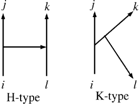
Figure 1: The two possible configurations Jacobi coordinates in the four-body problem are shown schematically.

H-type Jacobi coordinates are constructed by considering the separation vector for a pair of two-body subsystems, and the separation vector between the centers of mass of those two subsystems. Physically, H-type coordinates are useful for describing correlations between two particles, for example a two-body bound state or a symmetry between two particles, or two separate two-body correlations. K-type Jacobi coordinates are constructed in an iterative way by first constructing a three-body coordinate set as in Eq. (122), and then taking the separation vector between the fourth particle and the center of mass of the three particle sub-system. When two particles coalesce (e.g. when $\bm{r}_{i}=\bm{r}_{j}$ in Eq. 121), the H-type coordinate system reduces to a three-body system with two of the four particles acting like a single particle with the combined mass of its constituents. Locating these “coalescence points” on the surface of the hypersphere is crucial for an accurate description of the interactions between particles, and this coordinate reduction will prove useful for the construction of a variational basis set.

Examination of Fig. 1 shows that K-type Jacobi coordinate systems are useful for describing correlations between three particles within the four-particle system. In the four-fermion system, there are no weakly-bound trimer states, whereby K-type Jacobi coordinates will not be used here, but the methods described in this section can be readily generalized to include such states. Unless explicitly stated, all Jacobi coordinates from here on will be of the H-type.

The task of parametrizing the 3 Jacobi vectors in hyperspherical coordinates remains. There is no unique way of choosing this parameterization. The simplest method comes in the form of Delves coordinates. Construction of these hyperangular coordinates is outlined in Appendix A and is described in detail in a number of references (see Refs. Smirnov and Shitikova (1977a); Avery (1989) for example). This construction method also allows for a physically meaningful grouping of the cartesian coordinates. For example a hyperangular coordinate system that treats the dimer-atom-atom system as a separate three-body subsystem can be created. This type of physically meaningful coordinate system plays a crucial role in the construction of the variational basis set that follows.

After adoption of the Jacobi vectors, the center of mass of the four-body system is removed, which leaves a 9-dimensional partial differential equation to solve. By applying hyperspherical coordinates, this becomes an 8-dimensional hyperangular PDE that must be solved at each hyperradius, a daunting task. A further simplification is achieved by initially considering only zero total angular momentum states of the system. This implies that there is no dependence on the three Euler angles in the final wavefunction, and in a body-fixed coordinate system these three degrees of freedom can be removed. The body-fixed coordinates adopted here are called democratic coordinates, adequately described in several references (see Refs. Aquilanti and Cavalli (1997); Kuppermann (1997b); Littlejohn et al. (1999)). The parameterization of Aquilanti and Cavalli is convenient for our purposes (for more detail see their work in Ref. Aquilanti and Cavalli (1997)).

At the heart of democratic coordinates is a rotation from a space-fixed frame to a body-fixed frame:

$$\bm{\varrho}=\bm{D}^{T}\left(\alpha,\beta,\gamma\right)\bm{\varrho}_{bf}$$ (26)

where $\bm{\varrho}$ is the matrix of ”lab frame” Jacobi vectors defined in Eq. 132, $\bm{\varrho}_{bf}$ is the matrix of body-fixed Jacobi coordinates, and $\bm{D}\left(\alpha,\beta,\gamma\right)$ is an Euler rotation matrix defined in the standard way as

$$\bm{D}=\left[\begin{array}[c]{ccc}\cos\alpha&-\sin\alpha&0\\ \sin\alpha&\cos\alpha&0\\ 0&0&1\end{array}\right]\left[\begin{array}[c]{ccc}\cos\beta&0&\sin\beta\\ 0&1&0\\ -\sin\beta&0&\cos\beta\end{array}\right]\left[\begin{array}[c]{ccc}\cos\gamma&-\sin\gamma&0\\ \sin\gamma&\cos\gamma&0\\ 0&0&1\end{array}\right].$$ (27)

This parameterization is described in detail in Appendix A. After removing the Euler angles, the body fixed Jacobi vectors are then described by a set of $5$ angles $\left\{\Theta_{1},\Theta_{2},\Phi_{1},\Phi_{2},\Phi_{3}\right\}$ and the hyperradius $R$. The angles $\Theta_{1}$ and $\Theta_{2}$ parameterize the overall $x,$ $y,$ and $z$ spatial extent of the four-body system in the body-fixed frame, while the angles $\Phi_{1},$ $\Phi_{2},$ and $\Phi_{3}$ describe the internal configuration of the four particles.

The description of coalescence points in democratic coordinates is especially important. These are the points at which interactions occur and also where nodes must be enforced for symmetry. Figure 2 shows these points for $\Theta_{1}=\pi/2$, which enforces planar configurations, and for several values of $\Theta_{2}$. The body fixed coordinates in question are H-type Jacobi coordintes that connect identical fermions, so symmetry is is easily described. The $\Phi_{3}$ axis in Fig. 2 is shown from $\pi/2$ to $\pi$ and then $0$ to $\pi/2$ to emphasize symmetry. The red surfaces surround Pauli exclusion nodes while the blue surfaces surround interaction points. It is clear that using a symmetry-based coordinate system leaves a simple description of the Pauli exclusion nodes.

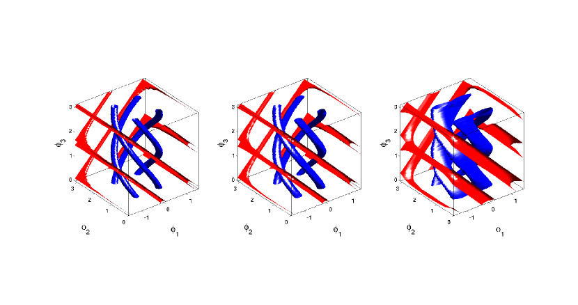
Figure 2: Surfaces surrounding the coalescence points in the body-fixed democratic coordinates are shown for $\theta_{1}=\pi/2$ and $\theta_{2}=\dfrac{\pi}{4}$ (a)$,\dfrac{\pi}{6}$ (b), and $\dfrac{\pi}{12}$ (c) respectively. Blue surfaces surround interaction coalescence points while red surfaces surround Pauli exclusion nodes.

III.1 Unsymmetrized basis functions

With the Jacobi vectors and democratic coordinates in hand, the 12-dimensional four-body problem is reduced to a 6-dimensional problem for total orbital angular momentum $J=0$. After the hyperradius is treated adiabatically, the remaining 5-dimensional hyperangular partial differential equation Eq. (2) must be solved at each $R$ to obtain the adiabatic channel functions and potentials used in the adiabatic hyperspherical representation. In Eq. (3), $\hat{V}(R;\Omega)$ is chosen as a sum of short-range pairwise interactions, which to an excellent approximation affects only the $s$-wave for each pair: $\hat{V}(R;\Omega)=\sum_{i,j}{\hat{V}\left(r_{ij}\right)}$, where the sum runs over all possible pairs of distinguishable fermions. This section only considers a potential whose zero energy s-wave scattering length $a$ is positive and large compared with the range $r_{0}$ of the interaction. Further, unless otherwise stated, we assume that the potential can support only a single weakly-bound dimer.

The strategy used here is not unknown Sadeghpour (1990). It involves using a variational basis that diagonalizes the adiabatic Hamiltonian in two limits asymptotically ($R\gg a$) and at small distances ($R\ll r_{0}$). It is thought that linear combinations of these basis elements will provide a variationally accurate description of the wavefunction at intermediate $R$-values.

Next we describe the unsymmetrized basis functions that exactly diagonalize Eq. (2) in the small-$R$ and large-$R$ regimes. At large $R$, three scattering thresholds arise: a threshold energy corresponding to weakly-bound dimers at twice the dimer binding energy, another threshold consisting of a single weakly bound dimer and two free particles, and finally a threshold associated with four free particles. In general, it would be necessary to consider another set of thresholds associated with trimer states plus a free atom (for instance, a set of Efimov states for bosons). But for equal mass fermions, such considerations are irrelevant since no weakly bound trimers occur in the $a\gg r_{0}$ regime. At small $R$, the physics is dominated by the kinetic energy, and the eigenstates of the adiabatic Hamiltonian are simply the 4-body hyperspherical harmonics which also describe four free particles at large $R$. For a detailed description of hyperspherical harmonics, see Appendix B. Identification of these threshold regimes gives a simple interpretation of the corresponding channel functions and provides a starting point for the construction of our variational basis.

III.1.1 Dimer-Atom-Atom Three-Body Basis Functions ($2+1+1$)

One fragmentation possibility that must be incorporated into the asymptotic behavior of the four-fermion system is that of an s-wave dimer with two free particles. The dimer wave function $\phi_{d}$ is best incorporated using a hyperangular parameterization that treats the dimer-atom-atom system with a set of three-body hyperangles, described by

$$\Psi^{\lambda_{3B}\mu_{3B}}\left(R,\Omega\right)=\phi_{d}\left(r_{12}\right)Y_{\lambda_{3B}\mu_{3B}}\left(\Omega_{3B}^{12}\right),$$ (28)

where $Y_{\lambda_{3B}\mu_{3B}}$ is a three-body hyperspherical harmonic defined in Eq. (99), $\lambda_{3B}$ is the three-body hyperangular momentum, and $\mu_{3B}$ indexes the degenerate states for each value of $\lambda_{3B}$. The dimer wave function $\phi_{d}$ is chosen as the bound state solution to the two-body Schrödinger equation:

$$\left[-\dfrac{\hbar^{2}}{2\mu_{2b}}\dfrac{\partial^{2}}{\partial r^{2}}+V\left(r\right)\right]r\phi_{d}\left(r\right)=-E_{b}r\phi_{d}\left(r\right).$$ (29)

Here the superscript $12$ in $\Omega_{3B}^{12}$ indicates that the third particle in the three-body subsystem is a dimer of particles 1 and 2. Further, for notational simplicity, $\mu_{3B}$ has been used to denote the set of quantum numbers, $\left\{l_{2},l_{3},m_{2},m_{3}\right\}$, which enumerate the degenerate states for each $\lambda_{3B}$.

So far the basis function defined by Eq. (28) is easily written in Delves coordinates. However, in order to ensure that $L$ is a good quantum number, one must couple the angular momenta corresponding to the interaction Jacobi coordinates $i1$ (defined in Eq. 130) to total angular momentum $L=0$. The angular momentum of the (s-wave) dimer is by definition zero and all that remains is to restrict the angular momentum of the three-body sub-system to zero. This can be achieved by recognizing that the angular momentum associated with the individual Jacobi vectors are good quantum numbers for the hyperspherical harmonics defined by Eq. (99), meaning that we can proceed using normal angular momentum coupling, i.e.

$$\Psi_{2+1+1}^{\lambda_{3B}l_{1}l_{2}}\left(R,\Omega\right)=\phi_{d}\left(r_{12}\right)\sum_{m_{2}=-l_{2}}^{l_{2}}\sum_{m_{3}=-l_{3}}^{l_{3}}\left\langle l_{2}m_{2}l_{3}m_{3}|00\right\rangle Y_{\lambda_{3B}\mu_{3B}}\left(\Omega_{3B}^{12}\right),$$ (30)

where $\left\langle l_{2}m_{2}l_{3}m_{3}|LM\right\rangle$ is a Clebsch-Gordan coefficient, and $l_{2}$ ($l_{3}$) is the angular momentum quantum number associated with $\bm{\rho}_{2}^{i1}$ ($\bm{\rho}_{3}^{i1}$) from the interaction Jacobi coordinates defined in Eqs. (130). Now with the total angular momentum set to $L=0$, there must be no Euler angle dependence in the total wavefunction. The Delves coordinates can then be defined for this system in the body fixed frame using Eq. (95). The Delves hyperangles are accordingly rewritten in terms of the democratic coordinates without including the Euler angle dependence.

III.1.2 Four-Body Basis Functions ($1+1+1+1$)

Another important asymptotic threshold that must be considered is that of four free particles. Using Delves coordinates, the free-particle eigenstates are four-body hyperspherical harmonics (see Appendix B):

$$\Phi_{\lambda\mu}^{\left(4b\right)}\left(\Omega\right)= N_{l_{l}l_{m}\lambda_{l,m}}^{33}N_{\lambda_{l,m}l_{n}}^{63}\sin^{\lambda_{l,m}}\left(\alpha_{lm,n}\right)\cos^{l_{n}}\left(\alpha_{lm,n}\right)P_{\left(\lambda-\lambda_{l,m}-l_{n}\right)/2}^{\lambda_{l,m}+5/2,l_{n}+1}\left(\cos 2\alpha_{lm,n}\right)$$

$$\times N_{l_{l},l_{m}}^{\lambda_{l,m}}\sin^{l_{l}}\left(\alpha_{l,m}\right)\cos^{l_{m}}\left(\alpha_{l,m}\right)P_{\left(\lambda_{l,m}-l_{l}-l_{m}\right)/2}^{l_{l}+1,l_{m}+1}\left(\cos 2\alpha_{l,m}\right)$$

$$\times Y_{l_{l}m_{l}}\left(\omega_{l}\right)Y_{l_{m}m_{m}}\left(\omega_{m}\right)Y_{l_{n}m_{n}}\left(\omega_{n}\right),$$

where $\mu$ has again been used to denote the set of quantum numbers $\left\{\lambda_{12},l_{1},l_{2},l_{3},m_{1},m_{2},m_{3}\right\}$ that enumerate the degenerate states for each $\lambda$. Here $l_{i}$ is the spatial angular momentum quantum number associated with the Jacobi vector $\bm{\rho}_{i}^{\sigma}$ with z-projection $m_{i}$, and $\lambda_{l,m}$ is the sub-hyperangular momentum quantum number associated with the sub-hyperangular tree in Fig. 32 (For example, $\lambda_{12}=l_{1}+l_{2}+2n_{12}$ where $n_{12}$ is a non-negative integer.) The hyperangles $\left\{\alpha_{lm,n},\alpha_{l,m}\right\}$ are defined here using Delves coordinates as described in Appendix A and $\omega_{n}$ refers to the spherical polar angles associated with the Jacobi vetor $\bm{\rho}_{n}$.

The choice of quantum numbers described above does not give the total orbital angular momentum of the four particle system as a good quantum number. To accomplish this, the three angular momenta of the Jacobi vectors must be coupled to a resultant total , in this case to $L=0$. This gives a variational basis function of the form

$$\Psi_{1+1+1+1}^{\lambda\lambda_{12}l_{1}l_{2}l_{3}}\left(\Omega\right) =\sum_{M_{12}=-L_{12}}^{L_{12}}\sum_{m_{3}=-l_{3}}^{l_{3}}\sum_{m_{2}=-l_{2}}^{l_{2}}\sum_{m_{1}=-l_{1}}^{l_{1}}\left\langle L_{12}M_{12}l_{3}m_{3}|00\right\rangle$$ (31)

$$\times\left\langle l_{1}m_{1}l_{2}m_{2}|L_{12}M_{12}\right\rangle\Phi_{\lambda\mu}^{\left(4b\right)}\left(\Omega\right).$$

Now that the total angular momentum is set to $L=0$ the same procedure used for the $\Psi_{2+1+1}^{\lambda_{3B}l_{1}l_{2}}$ basis functions can be employed. However, this time the hyperangular parameterization is defined using the symmetry Jacobi coordinates in Eqs. (123). Since there is no dependence on the Euler angles, the Jacobi coordinates can then be defined in the body-fixed frame.

III.1.3 Dimer-Dimer Basis Functions ($2+2$)

The asymptotic behavior of the two-component four-fermion system must include a description of two s-wave dimers separated by a large distance. To incorporate this behavior the variational basis must include a basis function of the form,

$$\Psi_{2+2}\left(R,\Omega\right)=\phi_{d}\left(r_{12}\right)\phi_{d}\left(r_{34}\right),$$ (32)

where the subscript 2+2 indicates the dimer-dimer nature of this function, and the dimer wavefunction, $\phi_{d}$, is given by the two-body Schrödinger equation. Here $\mu_{2b}$ is the reduced mass of the two distinguishable fermions, and $E_{b}\approx\hbar^{2}/2\mu_{2b}a^{2}$ is the binding energy of the weakly bound dimer. At first glance the right-hand side of Eq. (32) depends only implicitly on the hyperradius and hyperangles. To make this dependence explicit, Eqs. (108) and (113) are employed to extract $r_{12}\left(R,\Omega\right)$ and $r_{34}\left(R,\Omega\right)$. It can also be noted that the basis function, Eq. 32, does not respect the symmetry of the identical fermions, i.e. $P_{13}\Phi_{2+2}\neq-\Phi_{2+2}$. The antisymmetrization of the variational basis is discussed in the next section.

III.2 Symmetrizing the Variational Basis

The definitions of the basis functions developed in the previous subsection do not include the fermionic symmetry of the four particle system in question. Until this point, we have only been concerned with Jacobi coordinate systems in which the particle exchange symmetry is well described and with a single set of Jacobi vectors that describe some of the interactions. In order to impose the $S_{2}\otimes S_{2}$ symmetry of two sets of two identical fermions, we now incorporate the extra H-type Jacobi coordinates described in Appendix C. As a first step we define the projection operator,

$$\hat{P}=\dfrac{1}{4}\left(\hat{I}-\hat{P}_{13}\right)\left(\hat{I}-\hat{P}_{24}\right),$$ (33)

where $\hat{I}$ is the identity operator, and $\hat{P}_{ij}$ is the operator that permutes the coordinates of particles $i$ and $j.$ This operator will project any wavefunction onto the Hilbert space of wavefunctions that are antisymmetric under exchange of identical fermions. Since we are treating the fermionic species as distinguishable, permutations of members of different species are ignored. Applying this projection operator to the dimer-dimer basis function yields an unnormalized basis function,

$$\Psi_{2+2}^{\left(symm\right)}\left(R,\Omega\right)=\hat{P}\Psi_{2+2}\left(R,\Omega\right)=\dfrac{1}{2}\left(\phi_{d}\left(r_{12}\right)\phi_{d}\left(r_{34}\right)-\phi_{d}\left(r_{14}\right)\phi_{d}\left(r_{23}\right)\right),$$ (34)

where the inter-particle distances $r_{14}$ and $r_{23}$ are given in Eqs. (110) and (111).

Imposition of the antisymmetry constraints on the dimer-atom-atom basis functions in Eq. (30) yields

$$\Psi_{2+1+1}^{\left(symm\right)\lambda_{3b}l_{2}l_{3}}\left(R,\Omega\right) =\hat{P}\Psi_{2+1+1}^{\lambda_{3b}l_{2}l_{3}}\left(R,\Omega\right)$$

$$= \dfrac{1}{4}\phi_{d}\left(r_{12}\right)\sum_{m_{2}=-l_{2}}^{l_{2}}\sum_{m_{3}=-l_{3}}^{l_{3}}\left\langle l_{2}m_{2}l_{3}m_{3}|00\right\rangle Y_{\lambda_{3B}\mu_{3B}}\left(\Omega_{3B}^{12}\right)$$ (35)

$$-\dfrac{1}{4}\phi_{d}\left(r_{23}\right)\sum_{m_{2}=-l_{2}}^{l_{2}}\sum_{m_{3}=-l_{3}}^{l_{3}}\left\langle l_{2}m_{2}l_{3}m_{3}|00\right\rangle Y_{\lambda_{3B}\mu_{3B}}\left(\Omega_{3B}^{23}\right)$$

$$-\dfrac{1}{4}\phi_{d}\left(r_{14}\right)\sum_{m_{2}=-l_{2}}^{l_{2}}\sum_{m_{3}=-l_{3}}^{l_{3}}\left\langle l_{2}m_{2}l_{3}m_{3}|00\right\rangle Y_{\lambda_{3B}\mu_{3B}}\left(\Omega_{3B}^{14}\right)$$

$$+\dfrac{1}{4}\phi_{d}\left(r_{34}\right)\sum_{m_{2}=-l_{2}}^{l_{2}}\sum_{m_{3}=-l_{3}}^{l_{3}}\left\langle l_{2}m_{2}l_{3}m_{3}|00\right\rangle Y_{\lambda_{3B}\mu_{3B}}\left(\Omega_{3B}^{34}\right),$$

where $\Omega_{3B}^{ij}$ is the set of three-body hyperangles associated with particles $i$ and $j$ in a dimer and the remaining two particles free. The democratic parameterizations for the inter-particle distances from Eqs. (108)-(113) can be used in the dimer wavefunction directly. Through the use of symmetry coordinates, the hyperangles of the four-body system can be divided into a dimer subsystem and a three-body subsystem where the third particle is the dimer itself. Using the three-body hyperangles in the three-body harmonic in each term of Eq. (35), combined with the kinematic rotations from Eqs. (137) and (141), the three-body harmonics are then fully described in the hyperangles defined using symmetry Jacobi coordinates. Since $\Psi_{2+1+1}^{\left(symm\right)\lambda_{3b}l_{2}l_{3}}$ has been constrained to zero total spatial angular momentum, $L=0$, the body-fixed parameterization of the Jacobi vectors can be inserted directly without worrying about the Euler angles $\alpha,\beta$ and $\gamma$.

The final set of basis functions that must be antisymmetrized with respect to identical fermion exchange are the hyperspherical harmonics representing four free particles. Permutation of the identical fermions is accomplished in the symmetry coordinates using Eqs. (124)-(129). Using these permutations gives

$$\hat{P}_{13}\Psi_{1+1+1+1}^{\lambda\lambda_{12}l_{1}l_{2}l_{3}}\left(\Omega\right) =\left(-1\right)^{l_{1}}\Psi_{1+1+1+1}^{\lambda\lambda_{12}l_{1}l_{2}l_{3}}\left(\Omega\right),$$

$$\hat{P}_{24}\Psi_{1+1+1+1}^{\lambda\lambda_{12}l_{1}l_{2}l_{3}}\left(\Omega\right) =\left(-1\right)^{l_{2}}\Psi_{1+1+1+1}^{\lambda\lambda_{12}l_{1}l_{2}l_{3}}\left(\Omega\right),$$

where antisymmetry of the four free particle basis functions is enforced simply by choosing $l_{1}$ and $l_{2}$ to be odd.

Another symmetry in this system is that of inversion (parity), in which all Jacobi coordinates are sent to their negatives,

$$\bm{\rho}_{j}^{\sigma}\rightarrow-\bm{\rho}_{j}^{\sigma},$$

where $\sigma=s,i1,i2$ and $j=1,2,3$. Following the definitions of the Jacobi coordinates, positive inversion symmetry in the $1+1+1+1$ basis functions, $\Psi_{1+1+1+1}^{\lambda\lambda_{12}l_{1}l_{2}l_{3}}\left(\Omega\right)$, is imposed by choosing $\lambda$ to be even. The $2+1+1$ basis functions,$\Psi_{2+1+1}^{\left(symm\right)\lambda_{3b}l_{2}l_{3}}\left(R,\Omega\right)$, must already have positive inversion symmetry since $\phi_{d}\left(r\right)$ is an s-wave dimer wavefunction and $l_{2}=l_{3}$ for zero total spatial angular momentum, $L=0$. The dimer-dimer basis function, $\Psi_{2+2}^{\left(symm\right)}\left(R,\Omega\right)$, is already symmetric under inversion and does not need further restrictions placed on it.

The final symmetry to be imposed is not quite as obvious as the symmetries discussed so far. By performing a “spin-flip” operation in which the distinguishable species of fermions are exchanged, i.e. $\hat{P}_{12}\hat{P}_{34}$, the Hamiltonian in Eq. 3 (with $N=4$) remains unchanged. This operation is identical to inverting the two dimers in the dimer-dimer basis function. One can see that $\Psi_{2+2}^{\left(symm\right)}$ is unchanged under this operation. We will limit ourselves to dimer-dimer collisions in this section and will only be concerned with basis functions that have this symmetry. This symmetry is imposed on both $\Psi_{2+1+1}^{\left(symm\right)\lambda_{3b}l_{2}l_{3}}$ and $\Psi_{1+1+1+1}^{\lambda\lambda_{12}l_{1}l_{2}l_{3}}$ by demanding $l_{3}$ to be even.

Recalling that $\lambda=(l_{1}+l_{2}+2n_{1})+l_{3}+2n_{2}$ where $n_{1}$ and $n_{2}$ are both non-negative integers, the combination of these symmetries implies that the minimum $\lambda$ for $\Psi_{1+1+1+1}^{\lambda\lambda_{12}l_{1}l_{2}l_{3}}$ must be $\lambda_{min}=2$. This argument plays a pivotal role in determining the overall threshold scaling law for four-body recombination, as is discussed in Section II.2.

IV Correlated Gaussian and Correlated Gaussian Hyperspherical Method

IV.1 Correlated Gaussian method

In this Section, we discuss alternative numerical techniques to study the four-body problem. First, we present a powerful technique to describe few-body trapped systems where the solutions are expanded in correlated Gaussian (CG) basis set. Additional details regarding the CG basis set, including the evaluation of matrix elements, symmetrization, and basis set selection are discussed in Appendix D. We then present an innovative method which combines the adiabatic hyperspherical representation with the CG basis set and Stochastic Variational method (SVM). For additional information on the methods described in this section, see (von Stecher (2008); von Stecher and Greene (2009b)).

IV.1.1 General procedure

Different types of Gaussian basis functions have long been used in many different areas of physics. In particular, the usage of Gaussian basis functions is one of the key elements of the success of ab initio calculations in quantum chemistry. The idea of using an explicitly correlated Gaussian to solve quantum chemistry problems was introduced in 1960 by Boys Boys (1960) and Singer Singer (1960). The combination of a Gaussian basis and the stochastical variational method SVM was first introduced by Kukulin and Krasnopol’sky Kukulin and Krasnopol’sky (1977) in nuclear physics and was extensively used by Suzuki and Varga Varga and Suzuki (1996, 1995, 1997); Varga et al. (1994). These methods were also used to treat ultracold many-body Bose systems by Sorensen, Fedorov and Jensen Sørensen et al. (2005). A detailed discussion of both the SVM and CG methods can be found in a thesis by Sorensen Sørensen (2005) and, in particular, in Suzuki and Varga’s book Suzuki and Varga (1998). In the following, we present the CG method and its application to few-body trapped systems.

Consider a set of coordinate vectors that describe the system $\{\bm{x}_{1},...,\bm{x}_{N}\}$. In this method, the eigenstates are expanded in a set of basis functions,

$$\Psi(\bm{x}_{1},\cdots,\bm{x}_{N})=\sum_{A}C_{A}\,\Phi_{A}(\bm{x}_{1},\cdots,\bm{x}_{N})=\sum_{A}C_{A}\,\braket{\bm{x}_{1},\cdots,\bm{x}_{N}}{A}.$$ (36)

Here $A$ is a matrix with a set of parameters that characterize the basis function. In the second equality we have introduced a convenient ket notation. Solving the time-independent Schrödinger equation in this basis set reduces the problem to a diagonalization of the Hamiltonian matrix:

$$\bm{\mathcal{H}}\bm{C}_{i}=E_{i}\bm{\bm{\mathcal{O}}}\bm{C}_{i}$$ (37)

Here, $E_{i}$ are the energies of the eigenstates, $\bm{C}_{i}$ is a vector form with the coefficients $C_{A}$ and $\bm{\mathcal{H}}$ and $\bm{\mathcal{O}}$ are matrices whose elements are $\mathcal{H}_{BA}=\braket{B}{\mathcal{H}}{A}$ and $\mathcal{O}_{BA}=\braket{B}{A}$. For a 3D system, the evaluation of these matrix elements involves $3N$-dimensional integrations which are in general very expensive to compute. Therefore, the effectiveness of the basis set expansion method relies mainly on the appropriate selection of the basis functions. As we will see, the CG basis functions permit a fast evaluation of overlap and Hamiltonian matrix elements; they are flexible enough to correctly describe physical states.

To reduce the dimensionality of the problem we take advantage of its symmetry properties. Since the interactions considered are spherically symmetric, the total angular momentum, $J$, is a good quantum number, and here we restrict ourselves to $J=0$. Observe that if the basis functions only depend on the interparticle distances, then Eq. (36) only describes states with zero angular momentum and positive parity ($J^{\Pi}=0^{+}$). Furthermore, in the problems we consider, the center-of-mass motion decouples from the system. Thus the CG basis functions take the form

$$\Phi_{\{\alpha_{ij}\}}(\bm{x}_{1},\cdots,\bm{x}_{N})=\psi_{0}(\bm{R}_{CM})\mathcal{S}\left\{\exp\left(-\sum_{j>i=1}^{N}\alpha_{ij}r_{ij}^{2}/2\right)\right\},$$ (38)

where $\mathcal{S}$ is a symmetrization operator and $r_{ij}$ is the interparticle distance between particles $i$ and $j$. Here, $\psi_{0}$ is the ground state of the center-of-mass motion. For trapped systems, $\psi_{0}$ takes the form, $\psi_{0}(\bm{R}_{CM})=e^{-R_{CM}^{2}/2a_{ho}^{M}}$. Because of its simple Gaussian form, $\psi_{0}$ can be absorbed into the exponential factor. Thus, in a more general way, the basis function can be written in terms of a matrix $A$ that characterizes them,

$$\Phi_{A}(\bm{x}_{1},\bm{x}_{2},...,\bm{x}_{N})=\mathcal{S}\left\{\exp(-\frac{1}{2}\bm{x}^{T}.\bm{A}.\bm{x})\right\}=\mathcal{S}\left\{\exp(-\frac{1}{2}\sum_{j>i=1}^{N}A_{ij}\bm{x}_{i}.\bm{x}_{j})\right\},$$ (39)

where $\bm{x}=\{\bm{x}_{1},\bm{x}_{2},...,\bm{x}_{N}\}$ and $A$ is a symmetric matrix. The matrix elements $A_{ij}$ are determined by the $\alpha_{ij}$ (see Appendix D.3). Because of the simplicity of the basis functions, Eq. (38), the matrix elements of the Hamiltonian can be calculated analytically.

Analytical evaluation of the matrix elements is enabled by selecting the set of coordinates that simplifies the integrals. For basis functions of the form of Eq. (39), the matrix elements are characterized by a matrix $M$ in the exponential. Hence the matrix element integrand can be greatly simplified if we write it in terms of the coordinate eigenvectors that diagonalize that matrix $M$. This change of coordinates permits, in many cases, the analytical evaluation of the matrix elements. The matrix elements are explicitly evaluated in Appendices D.1 and D.2.

Two properties of the CG method are worth mentioning. First, the CG basis set is numerically linearly-dependent and over-complete, so a systematic increase in the number of basis functions will in principle converge to the exact eigenvalues Sørensen (2005). Secondly, the basis functions $\Phi_{A}$ are square-integrable only if the matrix $A$ is positive definite. We can further restrict the basis function by introducing real widths $d_{ij}$ such that $\alpha_{ij}=1/d_{ij}^{2}$ which ensures that $A$ is positive definite. Furthermore, these widths are proportional to the mean interparticle distances in each basis function. Thus, it is easy to select them after considering the physical length scales relevant to the problem. Even though we have restricted the Hilbert space with this transformation, we have numerical evidence that that the results converge to the exact eigenvalues.

The linear dependence in the basis set causes problems in the numerical diagonalization of the Hamiltonian matrix Eq. (37). Different ways to reduce or eliminate such problems are explained in the Appendix D.5.

Finally, we stress the importance of selecting an appropriate interaction potential. For the problems considered in this review, the interactions are expected to be characterized primarily by the scattering length, i.e., to be independent of the shape of the potential. We capitalize on that flexibility by choosing a model potential that permits rapid evaluation of the matrix elements. A Gaussian form,

$$V_{0}(r)=-d\exp\left(-\frac{r^{2}}{2r_{0}^{2}}\right),$$ (40)

is particularly suitable for this basis set choice. If the range $r_{0}$ is much smaller than the scattering length, then the interactions are effectively characterized only by the scattering length. The scattering length is tuned by changing the strength of the interaction potential, $d$, while the range, $r_{0}$, of the interaction potential remains unchanged. This is particularly convenient in this method since it implies that we only need to evaluate the matrix elements once and we can use them to solve the Schrödinger equation at any given potential strength ( or scattering length). Of course, this procedure will give accurate results only if the basis set is complete enough to describe the different configurations that appear at different scattering lengths.

In general, a simple version of this method includes four basic steps: generation of the basis set, evaluation of the matrix elements, elimination of the linear dependence, and evaluation of the spectrum. The stochastical variational method (SVM), briefly discussed in Appendix D.6, combines the first three of these steps in an optimization procedure where the basis functions are selected randomly.

IV.2 Correlated Gaussian Hyperspherical method

Several techniques have been developed to solve few-body systems in the last few decades Faddeev (1960); Suzuki and Varga (1998); Malfliet and Tjon (1969); Yakubovsky (1967 [Sov. J. Nucl. Phys. 5 937 (1967); Macek (1968). Among these methods, the Correlated Gaussian (CG) technique presented in the previous Section has proven to be capable of describing trapped few-body systems with short-range interactions. Because of the simplicity of the matrix element calculation, the CG method provides an accurate description of the ground and excited states up to $N=6$ particles Blume et al. (2007). However, CG can only describe bound states. For this reason, it is numerically convenient to treat trapped systems where all the states are quantized. The CG cannot (without substantial modifications) describe states above the continuum nor the rich behavior of atomic collisions such as dissociation and recombination.

The hyperspherical representation, on the other hand, provides an appropriate framework to treat the continuum. In the adiabatic hyperspherical representation (see Sec. II), the Hamiltonian is solved as a function of the hyperradius $R$, reducing the many-body Schrödinger equation to a single variable form with a set of coupled effective potentials. The asymptotic behavior of the potentials and the channels describe different dissociation or fragmentation pathways, providing a suitable framework for analyzing collision physics. However, the standard hyperspherical methods expand the channel functions in B-splines or finite element basis functions Pack and Parker (1987); Zhou et al. (1993); Esry et al. (1996); Suno et al. (2002), and the calculations become very computationally demanding for $N>3$ systems.

Ideally, we would like to combine the fast matrix element evaluation of the CG basis set with the capability of the hyperspherical framework to treat the continuum. Here, we explore how the CG basis set can be used within the adiabatic hyperspherical representation. We call the use of CG basis function to expand the channel functions in the hyperspherical framework the CG hyperspherical method (CGHS).

In the hyperspherical framework, matrix elements of the Hamiltonian must be evaluated at fixed $R$. To proceed, consider first how the matrix element evaluation is carried out in the standard CG approach

In the CG method, we select, for each matrix element evaluation, a set of coordinate vectors that simplifies the integration, i.e., the set of coordinate vectors that diagonalize the basis matrix $M$ which characterizes the matrix element (see Appendix D.3). The flexibility to choose the best set of coordinate vectors for each matrix element evaluation is key to the success of the CG method.

The optimal set of coordinate vectors are formally selected by making an orthogonal transformation from an initial set of vectors $\bm{x}=\{\bm{x}_{1},...,\bm{x}_{N}\}$ to a final set of vectors $\bm{y}=\{\bm{y}_{1},...,\bm{y}_{N}\}$: $\bm{x}\bm{T}=\bm{y}$, where $\bm{T}$ is the $N\times N$ orthogonal transformation matrix. The hyperspherical method is particularly suitable for such orthogonal transformations because the hyperradius $R$ is an invariant under them. Consider the hyperradius defined in terms of a set of mass-scaled Jacobi vectors Delves (1959, 1960); Suno et al. (2002); Mehta et al. (2007), $\bm{x}=\{\bm{x}_{1},...,\bm{x}_{N}\}$,

$$R^{2}=\sum_{i}\bm{x_{i}}^{2},$$ (41)

If we apply an orthogonal transformation to a new set of vectors $\bm{y}$, then

$$R^{2}=\sum_{i}\bm{x_{i}}^{2}=\bm{y}\bm{T}^{T}\bm{T}\bm{y}=\sum_{i}\bm{y_{i}}^{2}$$ (42)

where we have used that $\bm{T}^{T}\bm{T}=\bm{I}$, and $\bm{I}$ is the identity. Therefore, in the hyperspherical framework we can also select the most convenient set of coordinate vectors for each matrix element evaluation. This is the key to reducing the dimensionality of the matrix element integrals. One can view the flexibility afforded by such orthogonal transformations of the Jacobi vectors instead in terms of the hyperangles $\Omega$ that best simplify the evaluation of matrix elements.

As an example of how the dimensionality of matrix-elements is reduced, consider a three dimensional $N$-particle system in the center of mass frame and with zero orbital angular momentum ($J=0$). We will show that this technique reduces a $(3N-7)$-dimensional numerical integral Jav to a sum over ($N-3$)-dimensional numerical integrals (see Subsec. IV.2.1). Hence, for $N=3$ the matrix elements can be evaluated analytically, and the $N=4$ matrix elements require a sum of one-dimensional numerical integrations.

The next three subsections discuss the implementation of the CGHS. Many of the techniques used in the standard CG method can be directly used in the CGHS approach. For example, the selection and symmetrization of the basis function can be directly applied in the CGHS method. Also, the SVM method can be used to optimize the basis set at different values of the hyperradius $R$. Subsection IV.2.1 describes how the hyperangular Schrödinger equation (Eq. 43) can be solved using a CG basis set expansion and shows, as an example, how the unsymmetrized matrix elements can be calculated analytically for a four particle system. Finally, subsection IV.2.2 discusses the general implementation of this method.

IV.2.1 Expansion of the channel functions in a CG basis set and calculation of matrix elements

In the hyperspherical method (see Sec. II), channel functions are eigenfunctions of the adiabatic Hamiltonian $\mathcal{H}_{A}(R;\Omega)$,

$$\mathcal{H}_{A}(R;\Omega)\Phi_{\nu}(R;\Omega)=U_{\nu}(R)\Phi_{\nu}(R;\Omega).$$ (43)

The eigenvalues of this equation are the hyperspherical potential curves $U_{\nu}(R)$. The adiabatic Hamiltonian has the form,

$$\mathcal{H}_{A}(R;\Omega)=\frac{\hbar^{2}\Lambda^{2}}{2\mu R^{2}}+\frac{(d-1)(d-3)\hbar^{2}}{8\mu R^{2}}+V(R,\Omega).$$ (44)

Here, $d=3N_{J}$ where $N_{J}$ is the number of Jacobi vectors.

A standard way to solve Eq. (43) is to expand the channel functions in a basis,

$$\ket{\Phi_{\mu}(R;\Omega)}=\sum_{i}c_{\mu}^{i}(R)\ket{B_{i}(R;\Omega)}.$$ (45)

Here $\mu$ labels the channel functions and $\ket{B_{i}(R;\Omega)}$ are the CG basis functions [Eq. (39)] written in hyperspherical coordinates. With this expansion, Eq. (43) reduces to the generalized eigenvalue equation

$$\bm{\mathcal{H}}_{A}(R)\bm{c}_{\mu}=U_{\mu}(R)\bm{\mathcal{O}}(R)\bm{c}_{\mu}.$$ (46)

The vectors $\bm{c}_{\mu}=\{c_{\mu}^{1},...,c_{\mu}^{D}\}$, where $D$ is the dimension of the basis set. $\bm{\mathcal{H}}_{A}$ and $\bm{\mathcal{O}}$ are the Hamiltonian and overlap matrices whose matrix elements are given by

$$\mathcal{H}_{A}(R)_{ij}=\braket{\braket{B_{i}}{\mathcal{H}_{A}(R;\Omega)}{B_{j}}}{,}{}{CGHSME1}$$ (47)

$$\mathcal{O}(R)_{ij}=\braket{\braket{B_{i}}{B_{j}}}{.}$$ (48)

Efficient evaluation of the matrix elements, e.g. Eqs. (LABEL:CGHSME1) and (48), is essential for the optimization of the basis functions and the overall feasibility of the four-body calculations. Here, we demonstrate how to speed up the calculation by reducing the dimensionality of the numerical integrations involved in the matrix element evaluation.

Consider a four-body system described by three Jacobi vectors, $\bm{x}\equiv\{\bm{x}_{1},\bm{x}_{2},\bm{x}_{3}\}$, once the center-of-mass motion is decoupled. The overlap matrix elements between two unsymmetrized basis functions $\Phi_{A}$ and $\Phi_{B}$ (characterized by matrices $A$ and $B$ in the respective exponents) is significantly simplified if we change variables to the set of coordinates that diagonalize $A+B$. We call $\beta_{1}$, $\beta_{2}$ and $\beta_{3}$ the eigenvalues and $y\equiv\{\bm{y}_{1},\bm{y}_{2},\bm{y}_{3}\}$ are the eigenvectors of $A+B$. In this new coordinate basis set the overlap integrand takes the form

$$\Phi_{A}(\bm{x}_{1},\bm{x}_{2},\bm{x}_{3})\Phi_{B}(\bm{x}_{1},\bm{x}_{2},\bm{x}_{3})=\exp\left(-\frac{\beta_{1}y_{1}^{2}+\beta_{2}y_{2}^{2}+\beta_{3}y_{3}^{2}}{2}\right).$$ (49)

In this set of eigencoordinates, the integration over the polar angles of $\bm{y}_{i}$, vectors is easily carried out. To fix the hyperradius, we express the magnitude of the $\bm{y}_{i}$ vectors in spherical coordinates, i.e. $y_{1}=R\sin\theta\cos\phi$, $y_{2}=R\sin\theta\sin(\phi)$and $y_{3}=R\cos\theta$. In these coordinates the overlap matrix elements reads

$$\braket{B}{A}\Big{|}_{R}=(4\pi)^{3}\int\exp\left(-\frac{R^{2}(\beta_{1}\sin^{2}\theta\cos^{2}\phi+\beta_{2}\sin^{2}\theta\sin^{2}\phi+\beta_{3}\cos^{2}\theta)}{2}\right)\\ \sin^{5}\theta\cos^{2}\theta\cos^{2}\phi\sin^{2}\phi d\theta d\phi.$$ (50)

The integration over one of the angles can be carried out analytically. Introducing a variable dummy $y$, the overlap matrix element takes the form

$$\braket{B}{A}\Big{|}_{R}=\frac{(4\pi)^{3}\pi}{2R^{2}(\beta_{1}-\beta_{2})}\int_{0}^{1}\exp\left(-\frac{R^{2}}{4}[(\beta_{1}+\beta_{2})(1-y^{2})+2\beta_{3}y^{2}]\right)\\ I_{1}\left[R^{2}\frac{(\beta_{1}-\beta_{2})(1-y^{2})}{4}\right]y^{2}(1-y^{2})dy,$$ (51)

where $I_{1}$ is the modified Bessel function of the first kind.

To simplify the interaction matrix element evaluation, it is advantageous to use a Gaussian model potential as was used in the CG method. In this case, the interaction term can be evaluated in the same way as the overlap term since the interaction is also a Gaussian. Each pairwise interaction can be written as $V_{ij}=V_{0}\exp(-\frac{r_{ij}^{2}}{2d_{0}^{2}})=V_{0}\exp(-x^{T}.M^{(ij)}.x/(2d_{0}^{2}))$ (see Subsec. D.3 for the definition of $M^{(ij)}$). Therefore the interaction matrix element has the structure

$$\braket{B}{V_{ij}}{A}=V_{0}\int d\Omega\exp(-\frac{x^{T}.(A+B+M^{(ij)}/d_{0}^{2}).x}{2}).$$ (52)

This integration can be performed following the same steps used for the overlap matrix element. Equation (51) can be used directly if we multiply it by $V_{0}$, and $\beta_{1}$, $\beta_{2}$ and $\beta_{3}$ are replaced by the eigenvalues of $A+B+M^{(ij)}/d_{0}^{2}$. Note that for each pairwise interaction, the matrix $M^{(ij)}$ changes and requires a new evaluation of the eigenvalues.

The third term we need to evaluate is the hyperangular kinetic term at fixed $R$. This kinetic term is proportional to the grand angular momentum operator $\Lambda$, defined for the $N=3$ case as

$$\frac{\Lambda^{2}\hbar^{2}}{2\mu R^{2}}=-\sum_{i}\frac{\hbar^{2}\nabla_{i}^{2}}{2\mu}+\frac{\hbar^{2}}{2\mu}\frac{1}{R^{5}}\frac{\partial}{\partial R}R^{5}\frac{\partial}{\partial R}.$$ (53)

The expression can be formally written as

$$\mathcal{T}_{\Omega}=\mathcal{T}_{T}-\mathcal{T}_{R},$$ (54)

where

$$\mathcal{T}_{\Omega}=\frac{\Lambda^{2}\hbar^{2}}{2\mu R^{2}},\;\;\;\;\mathcal{T}_{T}=-\sum_{i}\frac{\hbar^{2}\nabla_{i}^{2}}{2\mu},\;\;\mbox{and}\;\;\mathcal{T}_{R}=-\frac{\hbar^{2}}{2\mu}\frac{1}{R^{5}}\frac{\partial}{\partial R}R^{5}\frac{\partial}{\partial R}.$$ (55)

In typical calculations, $\mathcal{T}_{\Omega}$ is evaluated by directly applying the corresponding derivatives in the hyperangles $\Omega$. However, in this case, it is convenient to evaluate $\mathcal{T}_{T}$ and $\mathcal{T}_{R}$ separately, since it is easier to differentiate over the Jacobi vectors and the hyperradius. These two matrix elements are not separately symmetric, but the angular kinetic energy matrix, i.e., the total kinetic energy minus the hyperradial kinetic energy, is symmetric. To obtain an explicitly symmetric operator, we symmetrize the operation $\braket{B}{\mathcal{T}_{\Omega}}{A}|_{R}=(\braket{B}{\mathcal{T}_{T}-\mathcal{T}_{R}}{A}|_{R}+\braket{A}{\mathcal{T}_{T}-\mathcal{T}_{R}}{B}|_{R})/2$ and obtain

$$\braket{B}{\mathcal{T}_{\Omega}}{A}\Big{|}_{R}=\frac{(4\pi)^{3}}{R^{8}}\int\exp\left(-\frac{\beta_{1}y_{1}^{2}+\beta_{2}y_{2}^{2}+\beta_{3}y_{3}^{2}}{2}\right)\Upsilon(y_{1},y_{2},y_{3})y_{1}^{2}y_{2}^{2}y_{3}^{2}dy_{1}dy_{2}dy_{3}\Big{|}_{R},$$ (56)

where

$$\Upsilon(y_{1},y_{2},y_{3})=\frac{1}{2}\left\{\sum_{i=1}^{3}\left[-3\beta_{i}+\left(\beta_{i}^{2}-2(A.B)_{ii}+\frac{\beta_{i}}{R^{2}}\right)y_{i}^{2}\right]\right.\\ \left.-\left(\sum_{i=1}^{3}\frac{\beta_{i}y_{i}^{2}}{R^{2}}\right)^{2}+\frac{\overline{(\bm{y}.\bm{A}.\bm{y})(\bm{y}.B.\bm{y})}}{R^{2}}\right\}.$$ (57)

It is easy to show that $(A.B)_{ii}=\sum_{j=1}^{3}a_{ij}b_{ij}$ since $A$ and $B$ are symmetric matrices. Here the bar sign indicates the integration over the angular degrees of freedom of $\bm{y}_{1}$, $\bm{y}_{2}$, and $\bm{y}_{3}$. We then divide the total result by $(4\pi)^{3}$. Making these integrations analytically we obtain

$$\overline{(\bm{y}.\bm{A}.\bm{y})(\bm{y}.B.\bm{y})}=\sum_{i=1}^{3}a_{ii}b_{ii}y_{i}^{4}+\sum_{i>j}^{3}\left(a_{ii}b_{jj}+b_{ii}a_{jj}+\frac{4}{3}a_{ij}b_{ij}\right)y_{i}^{2}y_{j}^{2}.$$ (58)

Rewriting the $y_{i}$ variables in spherical coordinates, we separate the hyperradial dependence in Eq. (56). As in Eq. (50), one of the angular integrations can be evaluated analytically and the final expression reduces to a one dimensional integral involving modified Bessel function of the first kind (see Ref. von Stecher (2008) for more details).

The matrix elements involved in the $P$ and $Q$ couplings can be evaluated by following the above strategy, and it also reduces to a one dimensional numerical integration. The symmetrization of the matrix elements is handled just as in the standard CG method and is described in Appendix D.1.

IV.2.2 General considerations

Many of the procedures of the standard CG method can be easily extended to the CGHS. The selection, symmetrization, and optimization of the basis set follow the the standard CG method (see Appendices D.1, D.3, D.4, D.5 and D.6). However, the evaluation of the unsymmetrized matrix elements at fixed $R$ is clearly different. Furthermore, the hyperangular Hamiltonian [Eq. 43] needs to solved at different hyperradii $R$.

There are several properties that make the CGHS method particularly efficient. For the model potential used, the scattering length is tuned by varying the potential depths of the two-body interaction. Therefore, as in the CG case, the matrix elements need only be calculated once; then they can be used for a wide range of scattering lengths. Of course, the basis set should be sufficiently complete to describe the relevant potential curves at all desired scattering length values.

The selection of the basis function generally depends on $R$. To avoid numerical problems, the mean hyperradius of each basis function $\braket{R}_{B}$ should be of the same order of the hyperradius $R$ in which the matrix elements are evaluated. We can ensure that $\braket{R}_{B}\sim R$ by selecting some (or all) the weights $d_{ij}$ to be of the order of $R$.

We consider two different optimization procedures. The first possible optimization procedure is the following: First, we select a few basis functions and optimized them to describe the lowest few hyperspherical harmonics. The widths of these basis functions are rescaled by $R$ at each hyperradius so that they represent the hyperspherical harmonics equally well at different hyperradii. These basis functions are used at all $R$, while the remaining are optimized at each $R$. Starting from small $R$ (of the order of the range of the potential), we optimize a set of basis functions. As $R$ is increased, the basis set is increased and reoptimized. At every $R$ step, only a fraction of the basis set is optimized, and those basis functions are selected randomly. After several $R$-steps, the basis set is increased.

Instead of optimizing the basis set at each $R$, one can alternatively try to create a complete basis set at large $R_{max}$. In this case, the basis functions should be complete enough to describe the lowest channel functions with interparticle distances varying from interaction range $r_{0}$ up to the hyperradius $R_{max}$. Such a basis set can be rescaled to any $R<R_{max}$ and should efficiently describe the channel functions at that $R$. The rescaling procedure is simply $d_{ij}/R=d_{ij}^{max}/R_{max}$. This procedure avoids the optimization at each $R$. Furthermore, the kinetic, overlap, and couplings matrix elements at $R$ are straightforwardly related to the ones at $R_{max}$. The interaction potential is the only matrix element that needs to be recalculated at each $R$. This property can be understood by dimensional analysis. The kinetic, overlap and couplings matrix elements only have a single length scale $R$, so a rescaling of the widths is simply related to a rescaling of the matrix elements. In contrast, the interaction potential introduces a new length scale, so the matrix elements depend on both $R$ and $d_{0}$, and the rescaling does not work.

These two choices, the complete basis set or the small optimized basis set, can be appropriate in different circumstances. If a large number of channels are needed, the complete basis method is often the best choice. But, if only a small number of channels are needed, then the optimized basis set might be more efficient.

The most convenient method we have found to optimize the basis functions in the four-boson and four-fermion problem is the following: First we select a hyperradius $R_{m}$ that is $R_{m}\approx 300\,d_{0}$ where the basis function will be initially optimized. The basis set is increased and optimized until the relevant potential curves are converged and, in that sense, the basis is complete. This basis is then rescaled, as proposed in the second optimization method, to all $R<R_{m}$. For $R>R_{m}$, it is too expensive to have a “complete” basis set. For that reason, we use the first optimization method to find a reliable description of the lowest potential curves.

Note that for standard correlated Gaussian calculations, the matrices $A$ and $B$ need to be positive definite. This condition restricts the Hilbert space to exponentially decaying functions. In the hyperspherical treatment, this is not necessary since the matrix elements are always calculated at fixed $R$, even for exponentially growing functions. This gives more flexibility in the choice of optimal basis functions.

V Application to the Four-Fermion Problem

This section presents our results for the four-body fermionic problem using the methods discussed in Sections III and IV. Our finite-energy calculations for elastic and inelastic processes are compared to established zero-energy results and are seen to exhibit significant qualitative and quantitative differences. Several properties of trapped four-fermion systems are also discussed, along with the connections between this few-body system and the many-body BEC-BCS crossover physics.

V.1 Four-fermion potentials and the dimer-dimer wavefunction

Calculation of the hyperradial potentials and channel functions using the variational basis method of Sec. III is conceptually simple. Matrix elements of the hyperangular part of the full Hamiltonian are required,

$$H_{ad}=\dfrac{\hbar^{2}}{2\mu}\dfrac{\Lambda^{2}}{R^{2}}+\sum_{i,j}V\left(r_{ij}\right),$$

where the sum runs over all interacting pairs of distinguishable fermions. Sec. III, considered the specific two-body interaction to be general, but required the two-body potential to support a weakly bound dimer state (and hence a positive scattering length much larger than the range of the interaction). At this point we adopt the so-called Pöschl-Teller potential,

$$V\left(r\right)=-\dfrac{U_{0}}{\cosh^{2}\left(r/r_{0}\right)},$$ (59)

where $r_{0}$ is the range of the interaction. Unless otherwise stated $U_{0}$ is tuned so that $V\left(r\right)$ gives the appropriate scattering length with only a single shallow bound state. This potential is adopted because the bound state wavefunctions and binding energies are known analytically Landau and Lifshitz (1981), but any two-body interaction could be used here, provided that one obtains the wavefunctions and energies numerically or analytically.

Application of the variational basis results in a generalized eigenvalue problem,

$$\bm{H}\left(R\right)\bm{x}_{\nu}\left(R\right)=U_{\nu}\left(R\right)\bm{S}\left(R\right)\bm{x}_{\nu}\left(R\right)$$ (60)

where $U_{\nu}\left(R\right)$ is the $\nu$-th adiabatic hyperradial potential, and $\bm{x}_{\nu}$ is the channel function expansion in the variational basis. The matrix elements of $\bm{H}$ are given by matrix elements of the adiabatic Hamiltonian at fixed hyperradius,

$${H}_{nm}=\left\langle\Psi_{n}\left|H_{ad}\right|\Psi_{m}\right\rangle.$$

Because the variational basis is not orthogonal, a real, symmetric overlap matrix, $\bm{S}$, appears in this matrix equation. While the method employed here is conceptually simple, the actual calculation of the matrix elements is numerically demanding because the interaction valleys in the hyperangular potential surface, $\sum_{i,j}V\left(r_{ij}\right)$, become localized into narrow cuts of the hyperangular space at large hyperradii. Further, examination of Fig. 2 shows that the locus of coalescence points where the interatomic potential is appreciable has a complicated structure in the five dimensional body-fixed hyperangular space. To accurately calculate the matrix elements in Eq. (60) numerically, a large number of integration points must be placed within the interaction valleys.

Despite all of these complications, the adiabatic potential can be found approximately. Figure 3 shows the full set of hyperradial potentials including the diagonal non-adiabatic correction (solid curves) calculated using $8$ variational basis elements: one $2+2$ element, four $2+1+1$ elements, and three $1+1+1+1$ elements. Also shown are the expectation values of the basis elements themselves, i.e. the diagonal of $H(R)$ from Eq. (60) (dashed curves). All calculations shown here are performed for $a=100r_{0}$. It is clear that the lowest potential curve converges very quickly with respect to the number of variational basis elements used. The lowest potentials converge well when only a few variational basis functions are included, while the higher potentials are somewhat suspect. According to the universal theory of zero-range interactions, the hyperspherical potential curves should only depend on $a$ in the regime where $a$ is the dominant length scale in the problem. Thus, in our finite range interaction calculations, the adiabatic potentials should become universal in the $R\gg r_{0}$ regime for large scattering lengths, i.e. $a\gg r_{0}$. In other words, the potentials should look the same when scaled by the scattering length and the binding energy, $U_{\nu}(R\gg r_{0})=(\hbar^{2}/ma^{2})u_{\nu}(R/a)$ where $u_{\nu}(x)$ is a universal function for the $\nu$th effective potential. Comparison with the potential curves computed in the correlated Gaussian method shows excellent agreement in the lowest dimer-dimer potential, and reasonable agreement for the lowest few dimer-atom-atom potentials von Stecher (2008).

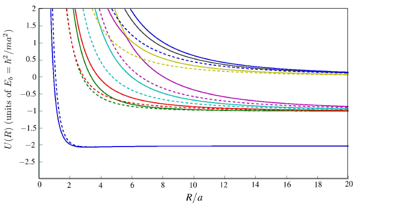
Figure 3: The calculated hyperradial potentials (solid lines) for $a=100r_{0}$ are shown as a function of $R/a$. Also shown are the expectation values of the fixed-$R$ Hamiltonian for the individual variational basis functions (dashed curves).

At large $R$, the lowest hyperradial adiabatic potential curve (see Fig. 3) approaches the bound-state energy of two dimers that are approximately separated by a distance $R$. It is natural to interpret processes for which flux enters and leaves this channel as ”dimer-dimer” collisions. Examining this potential further, one can see that at hyperradii less than the scattering length, $R<a$, the adiabatic dimer-dimer potential becomes strongly repulsive. This can be visualized qualitatively as hard wall scattering, which would give a dimer-dimer scattering length comparable to the two-body scattering length $a_{dd}\sim a$. Higher potential curves approach the single dimer binding energy at large $R$, indicating that these potentials correspond to a dimer with two free particles in the large $R$ limit. Note that the variational basis functions described in Section III give the correct large $R$ adiabatic energies by construction. As the scattering length becomes much larger than the range of the two-body potential, the effective four-fermion hyperradial potential becomes universal and independent of $a$. In the range of $r_{0}\ll R\ll a$:

$$U\left(R\right)\rightarrow\dfrac{\hbar^{2}}{2\mu}\dfrac{p_{0}^{2}-1/4}{R^{2}},$$ (61)

where $p_{0}=2.55$. This universal potential was extracted in Refs. von Stecher et al. (2007a, 2008b) by examining the behavior of the ground state energy of four fermions in a trap in the unitarity limit.

Figure 4 shows the coupling strengths, $\hbar^{2}P_{nm}^{2}/\left\{2\mu\left[\left(U_{m}\left(R\right)-U_{n}\left(R\right)\right)\right]\right\}$, between the dimer-dimer potential and the lowest three dimer-atom-atom adiabatic potentials for a two-body scattering length of $a=100r_{0}$. In each case the coupling strength peaks strongly near the short range region, $R\sim r_{0}$, and near the scattering length, $R\sim a$, and then falls off quickly in the large $R$ limit. This behavior indicates that recombination – from a state consisting of a dimer and two free particles to the dimer-dimer state – occurs mainly at hyperradii of the order of $a$. Looking at Fig. 4 one might think that a recombination path which occurs at small $R$, $R\sim r_{0}$, could also contribute, but the strong repulsion in the dimer-atom-atom potentials between $R\sim r_{0}$ and $R\sim a$, shown in Fig. 3, suppresses this pathway.

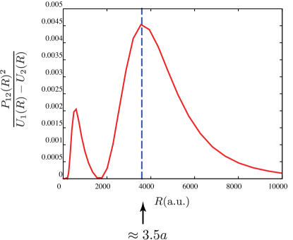
Figure 4: The nonadiabatic coupling strength between the dimer-dimer potential and the lowest dimer-atom-atom potential is shown as a function of $R$ ($r_{0}=100$ a.u. was choosen to be the van der Waals length of ${}^{4}0$K). The blue dashed line shows the position of the coupling peak at $R/a\approx 3.5$.

Figure 5 shows an isosurface of the hyperangular probability density in the configurational angles $\left\{\phi_{1},\phi_{2},\phi_{3}\right\}$ after integrating out $\Theta_{1}$ and $\Theta_{2}$ at a fixed hyperradius of $R=0.41a$. The $\phi_{1}$ axis has been modified here by shifting the region $\pi/2\leq\phi_{1}\leq\pi$ to emphasize the symmetry of the system. Each cobra-like surface corresponds to a peak in the four-body probability density. By examining Fig. 2, one sees that the spine of each cobra corresponds to the locus of interaction coalescence points. For each choice of $\left\{\phi_{1},\phi_{2},\phi_{3}\right\}$, the maximum of the probability density in $\Theta_{1}$ and $\Theta_{2}$ is given in a planar geometry, $\Theta_{1}=\pi/2$. The coloring of each cobra indicates the value of $\Theta_{2}$ at which the maximum occurs. Darker colors indicate a more linear geometry, i.e. $\Theta_{2}$ is closer to $0$. Figure 6 shows the same plot for the $2+2$ basis function only. A comparison of Figs. 5 and 6 indicates that the added variational basis elements are critical for describing the full dimer-dimer channel function for hyperradii less than the scattering length.

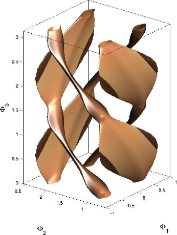
Figure 5: An isosurface of the dimer-dimer probability density is shown. The surfaces are found by integrating the total probability over $\theta_{1}$ and $\theta_{2}$ and plotting with respect to the remaining democratic angles $\left(\phi_{1},\phi_{2},\phi_{3}\right)$. The peak probability always occurs in planar configurations, $\theta_{1}=\pi/2$. The coloring (light to dark) indicates the value of $\theta_{2}$ at the peak.

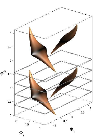
Figure 6: The same as Fig. 5, but using only the $2+2$ function. The dashed gray lines are purely for perspective.

V.2 Elastic dimer-dimer scattering

With the hyperradial potentials and non-adiabatic couplings in hand, low energy dimer-dimer scattering properties can be examined. The zero-energy dimer-dimer scattering length in the limit of large two-body scattering length was first calculated by Petrov et. al Petrov et al. (2004) and found to be

$$a_{dd}\left(0\right)=0.60\left(2\right)a,$$ (62)

where the number in the parentheses indicates $\pm 0.02$, the $2\%$ error stated in Ref. Petrov et al. (2004). This result has been confirmed using several different theoretical approaches Levinsen and Gurarie (2006); von Stecher et al. (2007a, 2008b); D’Incao et al. (2009a).

Using the adiabatic potentials shown in Fig. 3 and the resulting non-adiabatic couplings, the energy-dependent dimer-dimer scattering length defined by

$$a_{dd}\left(E_{\operatorname{col}}\right)=\dfrac{-\tan\delta_{dd}}{k_{dd}}$$ (63)

can be calculated. Here $E_{\operatorname{col}}$ is the collision energy of the two dimers with respect to the dimer-dimer threshold, and $\delta_{dd}$ is the s-wave dimer-dimer phase shift. When the collision energy becomes greater than the dimer binding energy, the two dimers collide with enough energy to potentially dissociate one of them. When this happens, the four fermion system can fragment in an excited hyperspherical channel causing a loss of flux from the dimer-dimer channel. This process is parameterized by the imaginary part of the dimer-dimer scattering length becomes non-zero when $E_{\operatorname{col}}>E_{b}$.

Figures 7 and 8 respectively show the real and imaginary parts of the dimer-dimer scattering length calculated with different numbers of adiabatic channels plotted as functions of $E_{\operatorname{col}}$ in units of the dimer binding energy. Also shown in Fig. 7 is the dimer-dimer scattering length calculated from the variational potential that results from using a single variational basis element. It is important to note that the single adiabatic channel calculation and the single basis function calculation are not the same. In the former, the single potential used is the lowest potential resulting from a calculation using multiple basis functions, while the latter is the result of using only the $2+2$ variational basis function and is guaranteed to be less accurate. Not surprisingly, the scattering length at collision energies comparable to the binding energy depends strongly on the number of channels used. With just a single channel in use, there is no decay pathway available for the system. As more channels are included the system has more pathways into which it can fragment, which modifies the high energy behavior.

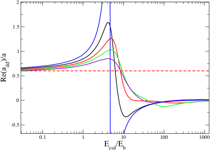
Figure 7: The real part of the energy dependent dimer-dimer scattering length is shown in units of the atom-atom scattering length $a$, plotted versus the collision energy in units of the dimer binding energy. The calculation is carried out with one, two, three, four, and five adiabatic channels (blue, black, red, green, and purple curves respectively) from the adiabatic potential curves and couplings computed using $8$ basis functions. The red dashed line shows $a_{dd}=0.6a$, the prediction of Ref. Petrov et al. (2005a).

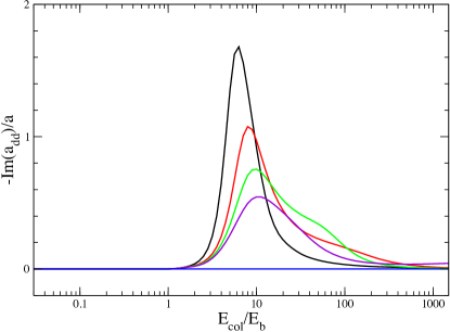
Figure 8: The imaginary part of the energy dependent dimer-dimer scattering length is shown in dimensions of $a$ plotted versus the collision energy in units of the binding energy. The calculation is carried out with one, two, three, four, and five adiabatic channels (blue, black, red, green, and purple curves respectively) from the adiabatic potential curves and couplings computed using $8$ basis functions.

What is more surprising is the low energy behavior seen in Fig. 7. For a single variational basis element, the dimer-dimer zero energy scattering length is found to be $a_{dd}=0.72a$, which is already within 20% of the result of Ref. Petrov et al. (2004), $a_{dd}\left(0\right)=0.6a$. A single channel calculation using the dimer-dimer potential and channel function that results from using 5 basis elements improves considerably on this yielding $a_{dd}\left(0\right)=0.64a$, showing that inclusion of correlations characteristic of two free particles at hyperradii less than $a$ gives a significant contribution to the physics of dimer-dimer scattering. It is somewhat unexpected that the single channel calculation is only $8\%$ off of the predicted value. As the scattering energy approaches zero, the higher fragmentation channels become strongly closed but still apparently play a small role in the dimer-dimer scattering process. By including progressively more channels in the scattering calculation the zero-energy dimer-dimer scattering length can be extracted for large two body scattering length:

$$a_{dd}\left(0\right)=0.605\left(5\right)a.$$ (64)

This result is in agreement with the results of Ref. von Stecher et al. (2007a, 2008b) and the results of Section V.6 which found the zero-energy dimer-dimer scattering length to similar accuracy using different methods.

V.3 Energy Dependent Dimer-Dimer Scattering

By examining the low energy behavior of the energy dependent dimer-dimer scattering length, the effective range can be extracted. The two dimers “see” each other when their wavefunctions are overlapping, i.e. when the hyperradius is approximately equal to the scattering length, $R\sim a$. If one thinks of the effective range of an interaction as proportional to the size of the interaction region, then one would expect the effective range for dimer-dimer scattering to be proportional to the scattering length. By fitting the low energy scattering phase shift to the effective range expansion,

$$\frac{-1}{a_{dd}(E)}=k_{dd}\cot\delta_{dd}=-\dfrac{1}{a_{dd}\left(0\right)}+\dfrac{1}{2}r_{dd}{k_{dd}}^{2}+\mathcal{O}({k_{dd}}^{4})$$ (65)

this intuitive behavior is born out, giving an effective range:

$$r_{dd}=0.13(1)a,$$ (66)

where $a$ is the two-body scattering length. Figure 9 shows both the real and imaginary parts of the energy dependent dimer-dimer scattering length as a function of collision energy in units of the binding energy compared to the effective range expansion, Eq. (65). This clearly shows that, while the low energy behavior of dimer-dimer scattering is well described by the effective range expansion, it is only accurate over a small range of collision energies. In fact, for collision energies larger than the binding energy, $a_{dd}\left(E_{\operatorname{col}}\right)$ actually turns over and decreases as dimer breakup channels become open. Further, when the collision energy exceeds the dimer binding energy, $E_{\operatorname{col}}=E_{b}$, the dimer-dimer scattering length becomes complex, with an imaginary part that parameterizes inelastic processes. These results indicate that both the real and imaginary dimer-dimer scattering lengths are universal functions of the collision energy. Specifically, they are insensitive to the short range nature of the two-body interaction, for scattering lengths much larger than the two-body interaction length scale, $r_{0}$. Because very few basis functions were used in these calculations, the results at higher energies, $E_{b}\ll E_{\operatorname{col}}\ll\hbar^{2}/mr_{0}^{2}$, are not well converged, though their qualitative nature is expected to persist. Well above the dissociation threshold, the real part of $a_{dd}$ exhibits an oscillatory behavior. These oscillations are caused by interference between different scattering pathways. As more basis functions are included and the high energy results converge, the large number of available pathways generally washes out the oscillatory behavior and produces incoherence , but the decrease in the real part of the $a_{dd}$ at higher energies is expected to survive as the calculations become better converged.

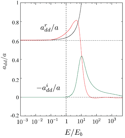
Figure 9: The real (red) and imaginary (green) parts of the energy dependent dimer-dimer scattering length are shown in units of $a$, plotted versus the collision energy in units of the binding energy. Also shown is the energy dependent scattering length predicted by the effective range expansion. Figure from Ref. D’Incao et al. (2009a).

The dependence of $a_{dd}$ on $a$ at finite collision energy is particularly interesting. In the large $a$ limit, the dimer binding energy becomes $E_{b}\approx\hbar^{2}/ma^{2}$, so that as $a$ increases, the binding energy decreases. At the critical value of the scattering length,

$$a_{c}=\dfrac{\hbar}{\sqrt{mE_{\operatorname{col}}}},$$

the collision energy coincides with the binding energy, and the dimer-atom-atom channel becomes open. As a result (see Fig. 9), one expects the real part of $a_{dd}$ to turn over and remain finite for all values of $a$. This behavior is demonstrated in Fig. 10 which compares the real part of the dimer-dimer scattering length at several fixed collision energies with the zero-energy result, $a_{dd}\left(0\right)=0.6a$. The scattering length scale has been fixed by setting the range of the interaction to be approximately the Van der Waals length of ⁴⁰K, $r_{0}\approx 100$ a.u. Another aspect of the finite collision energy behavior is that at large scattering length, the dimer-atom-atom channels become open, and dimer dissociation is allowed. Thus, near unitarity the Fermi gas might be viewed as a coherent mixture of atoms and weakly bound dimers.

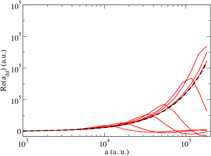
Figure 10: The real part of the energy dependent dimer-dimer scattering length is shown as a function of the two-body scattering length in atomic units for several collision energies: $E_{\operatorname{col}}/k_{b}=$250nK,100nK, 25nK, 10nK, 2.5nK, 1nK, $10^{-1}$nK, and $10^{-2}$nK. Also shown is the zero energy prediction (black dashed curve). Figure from Ref. D’Incao et al. (2009a).

V.4 Dimer-dimer relaxation

A significant loss process in an ultracold gas of bosonic dimers is that of dimer-dimer relaxation, in which two dimers collide and in the process at least one of the dimers relaxes to a deeply bound two-body state. The extra binding energy is released as kinetic energy which is sufficient to eject the remaining fragments from the trap. This process was studied by Petrov, Salomon and Shlyapnikov Petrov et al. (2004, 2005a), who assumed that the relaxation rate is controlled by the probability for three particles to be found in close proximity to one another. With this assumption and the further assumption that the fourth particle is far away and plays no role in the scattering process, they predict that the relaxation rate is suppressed at large two-body scattering lengths with a scaling law, $V_{rel}^{dd}\propto a^{-2.55}$.

Here we introduce a new method for finding the dimer-dimer relaxation rate based directly on Fermi’s golden rule. The key observation in this section is that the final allowed states appear as an infinite set of hyperspherical potentials corresponding to a deeply bound dimer with two free atoms. The transition rate to a single one of these potentials can be described by the Fermi-popularized golden rule, i.e.

$$T_{p}^{\lambda}\propto\left|\left\langle\Psi_{dd}\left(R;\Omega\right)\left|V\left(R,\Omega\right)\right|\Psi_{\lambda}\left(R,\Omega\right)\right\rangle\right|^{2}.$$ (67)

Here $\Psi_{\lambda}$ is the final outgoing state, $\Psi_{dd}$ is the dimer-dimer wavefunction, and $V\left(R,\Omega\right)$ is the sum of the two-body interactions. This matrix element and the sum of probabilities over final states are evaluated in Appendix E. The final result of this analysis is expressed as an integral over the hyperradius,

$$V_{rel}^{dd}\propto\int\dfrac{P_{WKB}\left(R\right)\mathcal{F}\left(R\right)}{R\kappa\left(R\right)}\rho\left(R\right)dR$$ (68)

where $P_{WKB}\left(R\right)$ is the WKB probability density of the dimer-dimer wavefunction at hyperradius $R$, $\kappa\left(R\right)$ is the WKB wavenumber:

$$\kappa\left(R\right)=\sqrt{\dfrac{2\mu}{\hbar^{2}}\left(V_{dd}\left(R\right)+\dfrac{\hbar^{2}}{2\mu}\dfrac{1/4}{R^{2}}-E_{\operatorname{col}}\right)}.$$ (69)

In Eq. (68) $\rho\left(R\right)$ is the nearly constant density of final states, and $\mathcal{F}\left(R\right)$ is the probability for three particles to be near one another in the dimer-dimer wavefunction at hyperradius $R$:

$$\mathcal{F}\left(R\right)=\left\langle\Phi_{dd}\left(R;\Omega\right)\left|f\left(R,\Omega\right)\right|\Phi_{dd}\left(R;\Omega\right)\right\rangle.$$ (70)

Here $\Phi_{dd}$ is the hyperangular dimer-dimer channel function, and $f\left(R,\Omega\right)$ is a proximity function that is appreciable only when three particles are all approximately within the range of the two-body interaction.

Equation (68) makes physical sense upon closer examination. It says that the rate at which a dimer relaxes to a deeper state is determined, with some extra factors, by the probability that three particles are close enough together so that two of them can fall into a deeply bound state and release the extra binding energy to the third particle. Figure 11 shows the integrand from Eq. (68) for several scattering lengths as a function of the hyperradius in units of the scattering length. This quantity can be interpreted as being proportional to the transition rate per unit hyperradius, i.e. the probability that the transition will occur between $R$ and $R+dR$. The full transition rate is determined by the nature of the interaction at short range and is not predictable using this method. By examining the relaxation rate as a function of scattering length, however, a scaling law can be extracted at each fixed hyperradius.

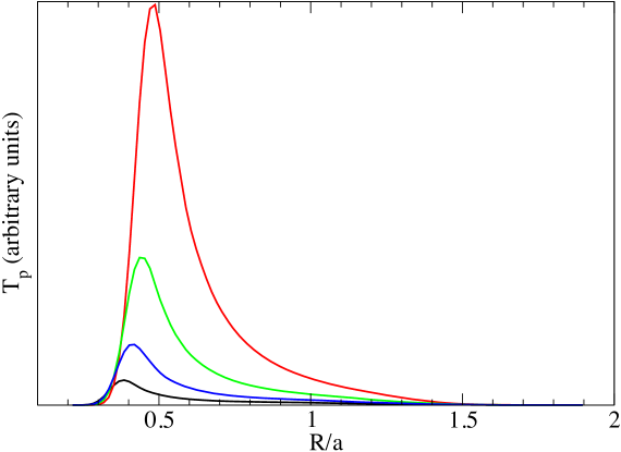
Figure 11: The integrand from Eq. (68) is shown for $a=50r_{0}$ (red),$64r_{0}$ (green),$80r_{0}$ (blue), and $100r_{0}$ (black) as a function of $R/a$.

Figure 12 shows the relaxation rate per unit hyperradius for several fixed values of $R/a$ as a function of the scattering length, $a$. The large $a$ behavior in each case appears to follow a scaling law, but the scaling law changes with $R/a$. This behavior indicates that, contrary to the prediction of Ref. Petrov et al. (2005a), when the integral in Eq. (68) is evaluated, the relaxation rate will not be determined by a simple power law. By integrating over different hyperradial regions, contributions to the transition rate from different processes can be extracted. For instance, if the integral in Eq. (68) is performed only over small hyperradii, $R\lesssim 5r_{0}$, the result is the transition rate due to processes in which all four particles are in close proximity. If the integral is evaluated over larger hyperradii, $R>10r_{0}$, the result is the rate due to three-body processes influenced by the presence of the fourth particle.

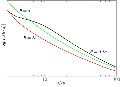
Figure 12: The logarithm of the integrand from Eq. (68) is shown for several fixed values of $R$ as a function of $a/r_{0}$

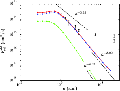
Figure 13: The relaxation rate in a dimer-dimer collision is shown as a function of the atom-atom scattering length (see text). Figure from Ref. D’Incao et al. (2009a)

Figure 13 shows the relaxation rate as a function of the scattering length in atomic units as a solid line. In this result the range of the interaction is set to the van der Waals length of ⁴⁰K, $r_{0}\approx 100$ a.u. Also shown in Fig. 13 are the contributions to this relaxation rate due to four-body processes (dashed blue curve), and due to three-body processes (dotted green curve). Also shown is the expected scaling law for transitions that occur at small hyperradius, $R=5r_{0}$. Because the hyperradius is small in this regime, the probability of three particles being in proximity is near unity, meaning that the transition probability per unit hyperradius is determined by the probability that the system can tunnel through the repulsive potential seen in Fig. 3 at $R\lesssim a$. The universal repulsive potential in this regime von Stecher (2008); D’Incao et al. (2009a),

$$U\left(R\right) =\dfrac{\hbar^{2}}{2\mu}\dfrac{p_{0}^{2}-1/4}{R^{2}},$$ (71)

$$p_{0} =2.55,$$ (72)

leads to a scaling law for transitions in the small $R$ regime that behaves as

$$V_{rel}^{dd}\propto a^{1-2p_{0}}=a^{-4.20}.$$ (73)

Figure 13 also shows the experimentally determined relaxation rates from Ref. Regal et al. (2004). Both the scaling law predicted in Ref. Petrov et al. (2005a) of $a^{-2.55}$ and the prediction using Eq. (68) are consistent with the experimental data in the regime for $1000$ a.u.$\lesssim a\lesssim 4000$ a.u.. The experimental data for $a>3000$ a.u. are in the regime where the average dimer separation is less than the dimer size, where the dimer-dimer scattering picture discussed here no longer applies.

V.5 Trapped four-body system

In this section we abandon the hyperspherical methods of the previous sections and examine the case of trapped four-fermion systems. The four-body system in confined geometries has recently become computationally accessible. In particular, the trapped two-component Fermi system has been intensely studied in the last few-years and has become a benchmark for different theories and universal predictions. One of the challenges present in the study of universal four-body physics in dilute gases with short range forces is the description of disparate length scales associated with the large interpaticle distances and the short-range two-body interactions.

In this section, we analyze the spectrum, dynamics and universal properties of four-body solutions in confined geometries. The four-body system is described by a the model Hamiltonian

$$H=\sum_{i=1}^{2}\left(\frac{-\hbar^{2}}{2m_{1}}\nabla_{i}^{2}+\frac{1}{2}m_{1}\omega^{2}\bm{r}_{i}^{2}\right)+\sum_{i^{\prime}=1}^{2}\left(\frac{-\hbar^{2}}{2m_{2}}\nabla_{i^{\prime}}^{2}+\frac{1}{2}m_{2}\omega^{2}\bm{r}_{i^{\prime}}^{2}\right)+\sum_{i=1}^{2}\sum_{i^{\prime}=1}^{2}V(r_{ii^{\prime}})$$ (74)

where unprimed indices label the fermionic species with mass $m_{1}$, primed indices label the species with mass $m_{2}$, and $\bm{r}_{i}$ is the position vector of the $i$th fermion. The trapping frequency $\omega$ is assumed to be equal for both species. In order to facilitate a calculation with the CG method described in Section IV, we take the interaction potential $V$ to be a purely attractive Gaussian (see Eq. (40)) and tune the depth of $V$ to give the desired (large) scattering length. The mass ratio $\kappa$ is defined by $m_{1}/m_{2}$, and throughout the analysis we assume $m_{1}\geq m_{2}$. A trap length $a_{ho}^{(i)}=\sqrt{\hbar/m_{i}\omega}$ is defined for each species as well as a trap length associated with the pair $a_{ho}=\sqrt{\hbar/2\mu\omega}$, where $\mu=m_{1}m_{2}/(m_{1}+m_{2})$. For equal mass systems, $a_{ho}=a_{ho}^{(1)}=a_{ho}^{(2)}$.

This section reviews a series of predictions for the two-component four-fermion system. The spectrum and structural properties of the four-fermion system are analyzed throughout the BCS-BEC crossover, followed by an exploration of the system dynamics as the scattering length is tuned close to a Fano-Feshbach resonance. Finally, we review a series of numerical studies that confirm and quantify universal predictions.

V.5.1 Spectrum in the BCS-BEC crossover

To obtain the $J=0$ spectra for the four-fermion system in the BCS-BEC crossover problem, the CG method (Section IV) is utilized to solve the time-independent Schrödinger equation for different values of $a$. Like most numerical methods, this method provides an adiabatic spectrum (in time), i.e., the energies of the spectrum are labeled according to their energy values as $a$ changes. The four-body spectra present a series of crossings or narrow avoided crossings when the scattering length is tuned across the BCS-BEC crossover. For this reason, it is convenient to use a representation where these narrow avoided crossings are treated diabatically, and the spectrum smoothly evolves from the BCS to the BEC side. The diabatic representation is more relevant from the physical point of view since the diabatic states are usually associated with good or “approximately good” symmetries of the problem.

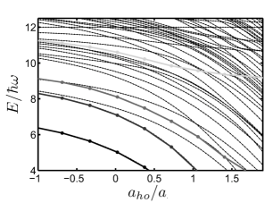
Figure 14: Four-fermion energy spectrum as a function of $\lambda=1/a$ in the unitarity region with $J=0$. The thin solid black lines correspond to the adiabatic spectrum. The wide black line with circles is the diabatic ground state labeled $\Psi_{DD1}$. The blue curve with circles is the diabatic first-excited state labeled $\Psi_{DD2}$, the wide red curve with circles is the diabatic state $\Psi_{DAA}$, and the wide green curve with circles is the diabatic state $\Psi_{4A}$.

To illustrate the diabatization procedure, consider the spectrum of the four-fermion system in the strongly interacting region shown in Fig. 14. A series of crossings and avoided crossings occurs when the adiabatic parameter $\lambda\equiv 1/a$ is varied in the strongly interacting region. The avoided crossings can be roughly characterized by their width $\Delta\lambda$, the range where the two adiabatic energy curves are coupled. There are narrow crossings where $\Delta\lambda\ll 1/a_{ho}$ and there are wide crossings where $\Delta\lambda\gtrsim 1/a_{ho}$. To obtain smooth energy values, we use variation of the diabatization procedure presented in Ref. Hesse et al. (2004).

The objective of the diabatization algorithm is to make the one-to-one connection between states and energies in consecutive points of the $\lambda$ grid that maximize the sum of the overlaps between connected states. The diabatization procedure starts from the BCS ($a<0$) side of the resonance and connects the states (and their energies) between consecutive values of $\lambda$ for which their overlap is maximum. When two initial energies connect to the same final energy, a refinement of the diabatization procedure is applied.

Diabatization is controlled by the spacing between consecutive values of $\lambda$ given by $\Delta\lambda_{g}$. If the width of the avoided crossing is smaller than $\Delta\lambda_{g}$, then that crossing is diabatized. But if the width of the avoided crossing is larger than $\Delta\lambda_{g}$, then that crossing is not diabatized. Thus, $\Delta\lambda_{g}$ is selected so that narrow crossings are diabatized and wide crossings remain adiabatic. For example, in Fig. 14 we see how this procedure diabatizes the narrow crossings of $\Psi_{4A}$, however, wide crossings such as the one between $\Psi_{DAA}$ and $\Psi_{4A}$ are still adiabatic in this representation.

This structure of avoided crossings permits a global view of the manner in which states evolve from weakly interacting fermions at $a<0$ to all the different configurations of a Fermi gas at $a>0$, i.e., molecular bosonic states, fermionic states, and molecular Bose-Fermi mixtures. Furthermore, it allow us to visualize concretely the alternative pathways of the time-dependent sweep experiments.

The diabatic spectrum of the four-fermion system is presented in Fig. 15. The structure of avoided crossings is complicated because of two different thresholds exist, one corresponding to the dimer-atom-atom and one to the dimer-dimer state. We identify three different families of diabatic states in this spectrum. The dimer-dimer family, represented by the black and blue curves, describes the ground and excited dimer-dimer states. These states are separated by approximately $2\hbar\omega$ on the BEC side. The dimer–two-atom family, represented by the red energy curves, follows the dimer binding energy. In the BEC limit, the dimer–two-atom family reproduces the degeneracies of three distinguishable particles: a spin up atom, a spin down atom, and a dimer. The third family describes four-atom bound states, for which the atoms form no dimers, and whose energy remains positive in the crossover region. In the BEC limit as $a\rightarrow 0$, the four-atom family reproduces the spectrum of the noninteracting four-body system.

The evolution of the $N=4$ spectra through the BCS-BEC crossover region can be understood qualitatively by considering the important quantum numbers for the description of the dimer. For each vibrational excitation of $2\hbar\omega$ in the noninteracting limit, there is one state that diabatically becomes a dimer-dimer state. These states correspond qualitatively to states where the relative angular momentum of two spin-up–spin-down pairs is zero [$L_{rel}^{\uparrow\downarrow}=0$], and the relative angular momentum between the pairs is also zero. The spin-up–spin-down pairs are in the lowest vibrational state. In the weakly interacting BCS limit, where the degeneracy of the vibrational states is broken, pair-pair states correspond to the lowest states.

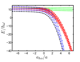
Figure 15: Energy spectrum for four particles with $J=0$ in the crossover region (lowest 20 diabatic states). The black curve corresponds to the ground state. The blue curves are the states that go diabatically to excited dimer-dimer configurations. The red curves correspond to states that connect diabatically to configurations of a dimer plus two free atoms, and the green curves correspond to states that connect diabatically to configurations of four free atoms. The lowest green curve is the atomic ground state on the BEC side of the resonance. Results from Ref. von Stecher and Greene (2007).

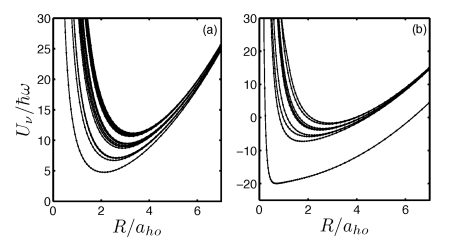
Figure 16: Hyperspherical potential curves in the BCS-BEC crossover for $N=4$ particles with $J=0$ angular momentum. (a) Potential curves in the BCS regime, $a\sim-0.3a_{ho}$. (b) Potential curves in the BEC regime, $a\sim 0.3a_{ho}$.

A direct and more concrete way to visualize the structure of the spectrum is to analyze the evolution of the adiabatic hyperspherical potential curves. Figure 16 presents the four-fermion adiabatic hyperspherical potential curves $U_{\nu}(R)$, obtained with the correlated Gaussian hyperspherical method (CGHS). Panel (a) presents the potential curves in the BCS regime, which are clearly grouped into families. Potential curves belonging to the same family are degenerate in the noninteracting limit. Thus, the weak interactions in the BCS regime break the degeneracies of the potential curves forming these families of potential curves. Panel (b) describes the system in the BEC regime. In this case, the description of the system is quite clear. The lowest potential curve is more than twice as deep as the rest of the curves and is associated with the dimer-dimer threshold. The family of dimer-dimer states live mainly in the lowest potential curve. The remainder of the displayed potential curves are associated with the dimer–two-atom threshold. The dimer–two-atom states are mainly described by this family of potential curves. A third family of potential curves, not shown in Fig. 16 (b), describes four-atom states. This family of potential curves has a different large-$R$ asymptotic behavior.

In order to benchmark the four-body energies, Figure 17 compares CG results with fixed-node diffusion Monte Carlo (FN-DMC) results carried out by Blume.von Stecher et al. (2007b) From the ground-state energy, the energy crossover curve $\Lambda_{4}^{(\kappa)}$, is constructed as in Refs. von Stecher et al. (2007b, 2008a):

$$\Lambda^{(\kappa)}=\frac{E(4)-2E(2)}{2\hbar\omega}.$$ (75)

Here $E(4)$ is the ground-state energy of the four-particle system and $E(2)$ is the ground-state energy of the two-particle system. By construction, the energy crossover curve $\Lambda_{4}^{(\kappa)}$ varies from 1 in the non-interacting–BCS regime ($a\to 0^{-}$) to 0 in the BEC limit ($a\to 0^{+}$). The energy crossover curve is convenient for comparisons because any effects of finite-range interactions on the two-body binding energy are significantly reduced by the subtraction in Eq. (75). Therefore, even though both $E(4)$ and $E(2)$ are not completely universal, $\Lambda_{4}^{(\kappa)}$ is universal to a very good approximation.

The solid lines in Figure 17 correspond to the CG prediction while the symbols correspond to the FN-DMC predictions obtained by Blume, for an equal mass system. To describe the four-fermion ground state with the FN-DMC method, two different guiding wave functions were used: a “normal” and a “paired” guiding function. The “normal” wave function can be written as the non-interacting solution multiplied by a Jastrow term that improves the description of short-range correlation. This guiding function is well suited to describe the ground state of the system in the BCS-unitarity regime. The “paired” wave function is constructed as an antisymmetrized product of two-body solutions and leads to a good description of the ground state in the BEC-unitarity regime. In order to reduce finite range corrections, the ranges $r_{0}$ of the two-body potentials used in Fig. 17 are set to be much smaller than the oscillator lengths, i.e., $r_{0}\approx 0.01a_{ho}^{(2\mu)}$. By analyzing the dependence of the energy on the finite range $r_{0}$, we can extrapolate the zero-range prediction and estimate the deviation in the crossover curve $\Lambda_{4}^{(\kappa)}$ from the zero range predictions. Such analysis estimates a 1% deviation in the crossover curve presented in Fig. 17. For example, at unitarity the CG energies are $E=5.027\hbar\omega$ for $r_{0}=0.01a_{ho}^{(2\mu)}$ and $E=5.099\hbar\omega$ for $r_{0}=0.05a_{ho}^{(2\mu)}$. After a more careful analysis of the range dependence we obtain an extrapolated zero-range value of $E=5.009\hbar\omega$. For comparison, the FN-DMC energy for the square well potential with $r_{0}=0.01a_{ho}^{(2\mu)}$ is $E=5.069(9)$, which agrees well with the energy calculated by the CG approach.

Figure 17: Energy crossover curve $\Lambda_{4}^{(\kappa)}$ as a function of $a_{ho}^{(2\mu)}/a$ for $\kappa=1$. Solid lines are calculated by the CG approach, and symbols by the FN-DMC method. Adapted from Ref. von Stecher et al. (2007b).

A test of the validity of the guiding function in FN-DMC calculations is fundamental for an accurate description of many-body fermionic systems. Comparisons, such as the one presented in Fig. 17 represent much-needed benchmark tests for the “normal” and “paired” trial wave-functions used in the FN-DMC approach von Stecher et al. (2007b) The good agreement between these two numerical methods suggests that, first, $\Lambda_{4}^{(\kappa)}$ is indeed universal; and second, that both numerical methods accurately describe the BCS-BEC crossover for this four-body system.

V.6 Extraction of dimer-dimer collisional properties

In the BEC limit, the lowest four body levels describe different vibrational states of a dimer-dimer configuration. Therefore, the systems can be treated effectively in this limit as two-particle systems. A comparison between the two particle solutions and the $N=4$ solutions allows us to extract information on the effective dimer-dimer interactions.

To model the effective dimer-dimer interaction we introduce a zero-range pseudopotential. Since the size of the dimers are of the order of $a$, the range of the effective potentials should also be of order of $a$. Accordingly, effective range effects are discussed using an energy-dependent scattering length. Inclusion of the scattering length energy dependence is well-known to extend the validity of the zero-range pseudopotential when applied to the scattering of two atoms with finite-range potentials under external confinement Blume and Greene (2002); Bolda et al. (2002). This energy dependence is included here through the effective range expansion

$$-\frac{1}{a_{dd}(E_{col})}\approx-\frac{1}{a_{dd}}+\frac{1}{2}k^{2}r_{dd}.$$ (76)

Here $a_{dd}(E_{col})$ is the energy-dependent dimer-dimer scattering length parameterized by the (zero-energy) scattering length $a_{dd}$ and the effective range $r_{dd}$. The momentum $k$ is associated with the relative kinetic energy of the dimer. Thus, $k^{2}/2\mu=E_{col}$ where $E_{col}=E_{4b}-2E_{2b}$. The appropriate reduced mass $\mu$ is $\mu_{dd}=M/2$, where $M$ is the mass of the bosonic molecules, $M=m_{1}+m_{2}$.

Using the effective range expansion [Eq. (65)], the regularized zero-range potential $V(r)$ Huang and Yang (1957) takes the form $V(r)=g(E)\delta(\bm{r})(\partial/\partial r)r$. The scattering strength $g$ is parameterized by the scattering length $a_{dd}$ and the effective range $r_{dd}$, i.e.,

$$g(E)=\frac{2\pi\hbar^{2}\,a_{dd}}{\mu}\left[1-\frac{\mu E_{col}r_{dd}a_{dd}}{\hbar^{2}}\right]^{-1}.$$ (77)

The $J=0$ spectrum of the two particle trapped system is given by Blume and Greene (2002); Bolda et al. (2002)

$$\sqrt{2}\frac{\Gamma\left(-\frac{E_{col}}{2\hbar\omega}+\frac{3}{4}\right)}{\Gamma\left(-\frac{E_{col}}{2\hbar\omega}+\frac{1}{4}\right)}=\frac{a_{ho}^{(\mu)}}{a_{dd}(E_{col})}.$$ (78)

Equation (78) is a transcendental equation that can be easily solved numerically. The solutions of Eq. (78) are obtained as functions of the $a_{dd}$ and $r_{dd}$ parameters and fitted to the numerical results. The calculation can be carried out at different values of the two-body scattering length $a$ and, in this way, one obtains a reliable estimation of $a_{dd}$ and $r_{dd}$.

Since the properties of weakly-bound dimers are controlled by the scattering length, it is natural to assume that the properties of dimer-dimer interactions are controlled only by $a$. This implies that $a_{dd}$ and $r_{dd}$ should be proportional to the two-body scattering length $a$. Therefore, we propose expressions of the form $a_{dd}=c_{dd}a$ and $r_{dd}=d_{dd}a$. The parameters $c_{dd}$ and $d_{dd}$ are obtained by fitting the zero-range two-particle solution to the dimer-dimer states of the $N=4$ system.

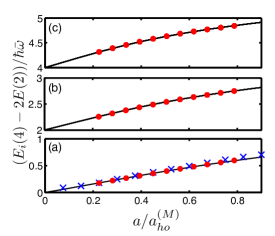
Figure 18: Four-body energies of the three energetically lowest-lying dimer-dimer states as a function of $a/a_{ho}^{(M)}$ for $\kappa=8$. Panel (a) shows the energetically lowest-lying energy level ($i=0$), panel (b) shows the energetically second-lowest ($i=1$) and panel (c) shows the energetically third-lowest state ($i=2$). Circles and crosses show our CG and FN-DMC results, respectively. Solid lines show the zero-range model results. Figure from Ref. von Stecher et al. (2007b).

The results in Fig. 18 illustrate the fitting procedure. The circles in Figs. 18(a)–(c) show the lowest-lying dimer-dimer energy levels, referred to as $E_{i}(4)$, where $i=0$–$2$ with the center-of-mass energy and the dimer-binding energy subtracted. These energies correspond to a two-heavy two-light four-body system with mass ratio $\kappa=8$. Solid lines represent the energy-dependent zero-range pseudopotential predictions obtained by fitting the two-boson model [Eq. (78)] to the four-body energies. The range of atom-atom scattering lengths, $a$, over which the four-fermion system can be described by the two-boson model is significantly extended by the inclusion of the effective range $r_{dd}$. Such inclusion also allows for a more stable and reliable determination of $a_{dd}$.

The crosses in Fig. 18(a) correspond to FN-DMC energies for the energetically lowest-lying dimer-dimer state. The Blume FN-DMC energies, presented in Ref. von Stecher et al. (2007b), are found to be slightly higher than the CG energies, the deviation increasing with $a$. This increasing deviation might be attributed to the variational implications of the fixed-node constraint. The functional form of the nodal surface used in the FN-DMC calculations was constructed for noninteracting dimers and should be best in the very deep BEC regime. Application of the two-boson model and the fitting procedure to the Blume FN-DMC energies provides an alternative determination of $a_{dd}$ and $r_{dd}$. The increasing deviation between the FN-DMC and CG energies with increasing $a$ explains why the effective range predicted by the analysis of the FN-DMC energies is somewhat larger than that predicted by the analysis of the CG approach (see discussion of Fig. 19 below).

The formation of few-body states, such as trimers or tetramers, can affect the scattering properties and limit the applicability of the two-boson model. For example, the lowest four-body energy for $\kappa=1$, constitutes the true ground state of the system, i.e., no energetically lower-lying bound trimer or tetramer states with $J^{\Pi}=0^{+}$ symmetry exist. However, for larger mass ratios, bound trimer and tetramer states exist. These few-body states can in principle be associated with either universal Efimov or nonuniversal physics. Even in the regime where few-body bound states exist, the four-body spectrum contains universal states that are separated by approximately $2\hbar\omega$ and are best described as two weakly-interacting composite bosons. For fixed $a$ ($a>0$), the energy of these “dimer-dimer states” changes smoothly as a function of $\kappa$ even in the regime where bound trimer states appear. Thus, our two-boson model and the fitting procedure can be extended to this regime of mass ratios.

Table 2 and Fig. 19 summarizes the dimer-dimer scattering length and effective range for for selected values of the mass ratio $\kappa$. Circles and crosses in Fig. 19 correspond to the dimer-dimer scattering length, $a_{dd}$, extracted from the energies calculated by the CG and the FN-DMC approach, respectively, as a function of $\kappa$. The $a_{dd}$ two-boson model predictions compare well with those calculated by Petrov et al. within a zero-range framework Petrov et al. (2005b) (solid line in Fig. 19). The existence of Efimov states limited Petrov et al. calculations to $\kappa\lesssim 13.6$ since beyond this mass ratio a three-body parameter is needed to solve the zero-range four-body equations. As mentioned above, the four-body solutions for a finite range potential include deeply-bound solutions which correspond to either a trimer-atom or a tetramer. The trimer-atom states affect the dimer-dimer scattering properties only when the dimer-dimer configuration is close in energy to the trimer-atom energy, which usually corresponds to a narrow window in two-body scattering length. Away from this window, the dimer-dimer states are well described by the two-boson mode which predicts a smooth increase of the $a_{dd}$ up to mass ratio $\kappa=20$.

Note that the existence of energetically-open atom-trimer channels at the dimer-dimer collisional energy provides a decay mechanism for the dimers. Clearly, such a decay mechanism cannot be captured within this rather simple two-boson model and a more sophisticated treatment should be used to extract the inelastic scattering properties.

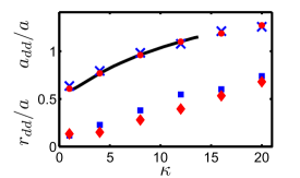
Figure 19: Circles and crosses show $a_{dd}/a$ as a function of $\kappa$ extracted from the four-fermion CG and FN-DMC energies, respectively. For comparison, a solid line shows the results from Fig. 3 of Ref. Petrov et al. (2005b). Diamonds and squares show $r_{dd}/a$ extracted from the four-fermion CG and FN-DMC energies, respectively. Figure from Ref. von Stecher et al. (2007b).

A recent theoretical study found good agreement with the two-boson model predictions beyond $13.6$ Marcelis et al. (2008).

Table 2: The dimer-dimer scattering length, $a_{dd}$, and dimer-dimer effective range, $r_{dd}$, obtained using (a) the CG spectrum and (b) the FN-DMC energies. The reported uncertainties reflect the uncertainties due to the fitting procedure; e.g., the potential limitations of the FN-DMC method to accurately describe the energetically lowest-lying gas-like stateare not included here (see Sec. IIIB of Ref. von Stecher et al. (2007b)).

$\kappa$	$a_{dd}/a$ (a)	$a_{dd}/a$ (b)	$r_{dd}/a$ (a)	$r_{dd}/a$ (b)
1	0.608(2)	0.64(1)	0.13(2)	0.12(4)
4	0.77(1)	0.79(1)	0.15(1)	0.23(1)
8	0.96(1)	0.98(1)	0.28(1)	0.38(2)
12	1.10(1)	1.08(2)	0.39(2)	0.55(2)
16	1.20(1)	1.21(3)	0.55(2)	0.60(5)
20	1.27(2)	1.26(5)	0.68(2)	0.74(5)

The two-boson model also provides estimates for the dimer-dimer effective range, $r_{dd}$ (shown as diamonds and squares in Fig. 19). The uncertainty of $r_{dd}$ obtained from the CG approach is estimated to be about 10%; this uncertainty is expected to be larger for the results extracted from the FN-DMC energies since those calculations only include one energy curve. As shown in Fig. 19, the ratio $r_{dd}/a$ increases from about 0.2 for $\kappa=1$ to about 0.5 for $\kappa=20$. The existence of a finite effective range can be attributed to the effective broad soft-core potential that the dimers experience Petrov et al. (2005b). Ref. von Stecher et al. (2007b) predicts $r_{dd}$ as a function of the mass ratio $\kappa$. The large value obtained for $r_{dd}$ suggests that effective-range corrections may need to be considered in order to accurately describe the physics of molecular Fermi gases.

To conclude, we have shown that studies of few-body trapped systems can be used to extract information about the collisional properties of free systems. Dimer-dimer scattering lengths can be extracted by analyzing the trapped few-body spectrum for different two-body scattering length values. Furthermore, energy-dependent corrections to $a_{dd}$ can also be obtained with this method.

V.7 Structural properties

The analysis of the BCS-BEC crossover spectrum can be complemented by an analysis of the wave functions and their structural properties. The present section determines the one-body densities and pair-distribution functions for two-component Fermi systems in the crossover regime. The averaged radial densities, $\rho_{i}(r)$, are normalized such that $4\pi\int\rho_{i}(r)r^{2}dr=1$; $4\pi r^{2}\rho_{i}(r)$ represents the probability of finding a particle with mass $m_{i}$ at a distance $r$ from the center of the trap. Here we focus in the $m_{1}=m_{2}$ case, where we find that the radial one-body densities $\rho_{1}(r)$ and $\rho_{2}(r)$ coincide and we can omit the species label. The unequal mass case, in which the radial one-body densities $\rho_{1}(r)$ and $\rho_{2}(r)$ differ, will not be considered here but was discussed in Ref. von Stecher et al. (2008b). Also, the averaged radial pair distribution functions, $P_{ij}(r)$, are normalized so that $4\pi\int P_{ij}(r)r^{2}dr=1$; $4\pi r^{2}P_{ij}(r)$ represents the probability of finding a particle of mass $m_{i}$ and a particle of mass $m_{j}$ at a distance $r$ from each other.

These structural properties are computed using the CG method. Since we are only focusing $J=0$ states, all the structural properties presented here are spherically symmetric. The structural properties are calculated using the following general expression:

$$4\pi r^{2}F(r)=\braket{\Psi_{n}}{\delta(x-r)}{\Psi_{n}}=\int d\bm{r}_{1}...d\bm{r}_{N}\delta(x-r)|\Psi_{n}(\bm{r}_{1},\bm{r}_{1^{\prime}},...,\bm{r}_{N_{1}},\bm{r}_{N_{2}})|^{2}.$$ (79)

Here, $F(r)$ is a generic structural property, e.g. the density profiles $\rho_{1}$ or $\rho_{2}$, the interspecies pair-correlation function $P_{12}$, or the intraspecies pair-correlation functions $P_{11}$ or $P_{22}$. $x$ is the length of the coordinate vector that describes the structural property. For $\rho_{1}$ and $\rho_{2}$, $x=r_{1}$ and $x=r_{1^{\prime}}$, respectively. For $P_{12}$, $x$ is the interparticle distance between opposite-spin or different species, $x=r_{11^{\prime}}$. For $P_{11}$ and $P_{22}$, $x$ is the same-spin or same-species interparticle distance, with $x=r_{12}$ and $x=r_{1^{\prime}2^{\prime}}$, respectively. To evaluate $4\pi r^{2}F(r)$, $\Psi_{n}$ is expanded in the CG basis set, permitting the integral in Eq. (79) to be carried out analytically.

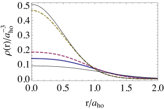
Figure 20: Single particle density profiles for interaction strength across the crossover. Thick curves correspond to numerical results: $a=-a_{ho}$ (solid curves), $a=\pm\infty$ (dashed curves) and $a=0.1a_{ho}$ (dash-dotted curves). Thin curves correspond to analytic limiting solutions: noninteracting four-fermion prediction (less peaked), dimer-dimer solution in the BEC limit (more peaked).

Figure 20 presents the single particle density profiles for different interaction strength across the crossover. The radial density profiles of the equal mass four-fermion system smoothly evolve from the noninteracting solution (less peaked thin black curve) in the BCS limit to the prediction of dimer-dimer model in the BEC limit (more peaked thin black line). In the BEC limit ($a\to 0^{+}$), the density profile coincides with that of two point like bosonic dimers, i.e., $\rho(r)=\exp(-r^{2}/a_{ho}^{(M)})/(a_{ho}^{(M)}\sqrt{\pi})^{3}$. For small but finite positive scattering lengths (dash-dotted curve), the density profiles is broader which can be attributed to both the finite size of the dimers and the effective repulsive dimer-dimer interaction.

Next, we analyze the opposite-spin pair distribution function. For a zero-range pseudopotential, the opposite-spin pair-correlation function obeys a boundary condition Lobo et al. (2006); Giorgini et al. (2008)

$$\frac{[rP_{12}(r)]^{\prime}_{r=0}}{[rP_{12}(r)]_{r=0}}=-\frac{2}{a}.$$ (80)

This behavior is a direct consequence of the Bethe-Peierls (B-P) boundary condition $[r_{12}\Psi(r_{12})]^{\prime}_{r_{12}=0}/[r_{12}\Psi(r_{12})]_{r_{12}=0}=-1/a$. The factor of 2 in Eq. (80) appears because the pair correlation function is proportional to the square of the wave function, i.e., $P_{12}(r)\propto\Psi(r_{12})^{2}$. A direct consequence of Eq. (80) is that at unitarity, i.e., when $|a|=\infty$, $r^{2}P_{12}(r)$ has zero slope at $r\rightarrow 0$.

Figure 21: Pair-distribution functions $P_{12}(r)$, multiplied by $r^{2}$, for equal-mass–two-component Fermi systems with $N=2$ (dashed curve) and $N=4$ (solid curve). The $N=2$ pair-correlation function has an arbitrary norm selected to match the $N=4$ pair correlation in the small $r$ regime.

The numerical verification of Eq. (80) is challenging. For systems with finite range interactions, Eq. (80) is valid in a narrow regime of $r$ values. For $a<0$, Eq. (80) is valid when $r$ is much larger than the range of the potential and much smaller than the mean interparticle distance, i.e., the $r_{0}\ll r\ll a_{ho}$ regime. For $a>0$, Eq. (80) is valid when $r$ is much larger than the range of the potential and much smaller than the size of the dimer (given by $a$) and the mean interparticle distance, i.e., the $r_{0}\ll r\ll\mbox{min}[a,a_{ho}]$ regime. This regime is almost nonexistent for our numerical calculations, because we consider only the $a_{ho}/r_{0}=100$ case.

The pair distribution function changes considerably as interactions are tuned across the BCS-BEC crossover. Figure 22 shows the pair distribution function $P_{12}(r)$ along the crossover for equal mass systems [$\kappa=1$] in the BCS (solid lines), unitary (dashed lines) and BEC (dash-dotted lines) regime. As attractive interactions increase, the pair distribution function evolves from a single peak structure to a double peak structure. The single peak structure is usually associated to solutions where spin-up-spin-down interparticle distances are mainly controlled by a single length scale and all particles are roughly at the same distance. This single peak structure appears in the BCS regime since the attraction is not strong enough to bind the particles and the typical interparticle distance is set mainly by the external trapping potential. The multi peak structures in pair distribution functions are generally associated to solutions were more than one length scale control the interspecies interparticle distance. In this case, a double peak structure already appears at unitarity and becomes more pronounce in the BEC regime. The peak at small $r$ indicates the formation of weakly bound dimers and its width is associated to the size of the dimers. The broader peak between $1\,a_{ho}$ and $2\,a_{ho}$ is related to the presence of larger atom-atom length scales set approximately by the typical dimer-dimer separation in the harmonic oscillator potential. Understanding the BEC solutions as two dimers in a trap implies that the four-body configurations includes two interspecies distances of the size of the dimer (short) and two interspecies distances of the size of the trap (large). Thus, the probability of finding two particles from different species at short distances should be equal to the probability of finding them at large distances. This premise can is verified by comparing the area under first and second peaks in the $P_{12}(r)r^{2}$ plot. Finally, note that in moving through the BCS-BEC crossover region, the slope of $r^{2}P_{12}(r)$ at small $r$ changes from positive to zero to negative, as is predicted by Eq. (80).

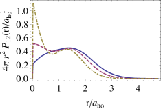
Figure 22: Pair-distribution functions $P_{12}(r)$, multiplied by $r^{2}$, for equal-mass–two-component Fermi systems with $N=4$ and $J=0$. The solid curve corresponds to $a=-a_{ho}$ (BCS regime), dashed curve $1/a=0$ (unitarity), and dashed-dotted $a=a_{ho}$ (BEC regime). Adapted from Ref. von Stecher et al. (2008a).

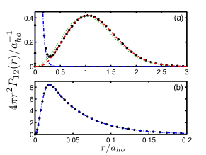
Figure 23: (a) Circles show the pair-distribution function, $P_{12}(r)$, multiplied by $r^{2}$, for $a=0.1a_{ho}$ (BEC regime). For comparison, the blue dash-dotted line shows $P_{12}(r)r^{2}$ for two atoms of mass $m$ with the same scattering length but normalized to $1/2$, the red dashed line shows $P_{12}(r)r^{2}$ for two trapped bosonic molecules of mass $2\,m$ interacting through a repulsive effective potential with $a_{dd}=0.6a$, and the green dotted line shows $P_{12}(r)r^{2}$ for two trapped noninteracting bosonic molecules of mass $2\,m$. Panel (b) shows a blow-up of the small $r$ region. Figure from Ref. von Stecher et al. (2008a).

The dimer-dimer model can be quantitatively tested in the deep BEC regime ($0<a\ll a_{ho}$). In this regime, the two peaks of the pair distribution function are well separated and can be independently analyzed. The small-$r$ corresponds to dimer formation and is well described by the pair-distribution function multiplied by $r^{2}$ and normalized to $1/2$, for two trapped atoms with $a=0.1a_{ho}$ (dash-dotted curve). The large-$r$ peak describes dimer-dimer correlations and is well described by the pair distribution function of two bosonic molecules of mass $2m$ in a harmonic trap (dotted line). The agreement is quite good but it can be improved by including the effective dimer-dimer interaction corrections. The dashed curve, almost indistinguishable from the large $r$ part of the pair-distribution function for the four-particle system, shows dimer-dimer model prediction including the effective repulsive potential with dimer-dimer scattering length $a_{dd}\approx 0.6a$ Petrov et al. (2005b); von Stecher et al. (2007b). Thus, even though the dimer-dimer interaction corrections are small, they are noticeably in the pair distribution function.

V.7.1 Dynamics across the BCS-BEC crossover region

The diabatic representation can be used to ramp an initial configuration through the BCS-BEC crossover region, mimicking experiments carried out at different laboratories at JILA and Rice University. The initial configuration is propagated using the time-dependent Schrödinger equation,

$$i\hbar\frac{d\ket{\Psi}}{dt}=\mathcal{H}[\lambda(t)]\ket{\Psi}.$$ (81)

The time dependence of the Hamiltonian comes entirely from that of $\lambda(t)\equiv 1/a(t)$ term. In this case, we focus on unidirectional ramps. Starting from the ground state on the BCS side, the parameter $\lambda$ is ramped through the resonance to the BEC side at different speeds, $\nu=\frac{d\lambda}{dt}$. The relevant dimensionless speed quantity is $\xi=a_{ho}\nu/\omega$. The parameter $\xi$ can be rewritten in terms of $\nu$, the density of the system $\rho$ and the particle mass to relate few-body and many-body predictions Borca et al. (2003). This reformulated version of $\xi$ (see Ref. von Stecher and Greene (2007)) agrees with the functional form of the Landau-Zener parameter obtained in Refs. Goral et al. (2004); Williams et al. (2006). The dependence of the Landau-Zener parameter on $\rho$ has been experimentally verified Hodby et al. (2005).

To propagate the initial configuration, we use the diabatic representation obtained previously in Sec V.5.1. First, we divide the BCS-BEC crossover range into sectors. Starting from the BCS side at $\lambda\approx\lambda_{BCS}$ and finishing at the BEC side at $\lambda\approx\lambda_{BEC}$, the BCS-BEC crossover is divided into 40–80 sectors. At the middle of each sector, the time-independent Hamiltonian is diagonalized using the CG method. For four-body systems, thousands of CG basis functions are usually needed to describe the spectrum. While in principle this basis set could be used to solve Eq. (81), in practice this large basis would make the numerical propagation very slow. Instead, we use the diabatic representation obtained at the middle of the $j$-th sector to expand the time-dependent wave function throughout that sector, i.e.,

$$\ket{\Psi(t)}=\sum_{i}^{N_{d}}c_{i}^{j}(t)\ket{\Psi^{j}_{i}}.$$ (82)

Here, $\ket{\Psi^{j}_{i}}$ is the diabatic basis function $i$ of sector $j$, and $N_{d}$ is the number of diabatic states considered. The time dependence only appears in the complex coefficients $c_{i}^{j}(t)$. Upon selecting only the lowest 20–100 diabatic states at that point, we drastically reduce the size of the Hamiltonian matrix in Eq. (81). Since the inverse scattering length $\lambda$ changes very little in each sector, the relevant diabatic states are well described by this reduced basis set throughout the sector. The time-dependent Schrödinger equation, Eq. (81), is propagated from one edge of the sector to the other using an adaptive-step Runge-Kutta method.

To understand the time propagation of this system, consider the way the probabilities evolve as the system transits the BCS-BEC crossover region. At each point of the time propagation, the probability to reside in state $i$ is given by $p_{i}(t)=|c_{i}^{j}(t)|^{2}$. Here $j$ denotes the sector that includes $\lambda(t)$. The probabilities of evolving into a given family can be found by summing the probabilities of all states belonging to the same family. For two particles, there are two families, the dimer family, which only includes the lowest state, and the two-atom family, which includes the rest of the states. In this case, the appropriate definitions are $p_{d}(t)=|c_{1}^{j}(t)|^{2}$, and $P_{2a}(t)=\sum_{i=2}^{N_{d}}|c_{i}^{j}(t)|^{2}$.

The $N=4$ system has four relevant families: the ground state, the excited dimer-dimer states, the dimer–two-atom states, and the four-atom states. These families are characterized by the probabilities $p_{g}(t)$, $p_{dd}(t)$, $p_{d2a}(t)$, and $p_{4a}(t)$, respectively.

Figure 24: Probabilities of different families of the $N=4$ system during a unidirectional ramp at constant speed $d\lambda/dt$ from the BCS to the BEC side. The initial configuration is $\ket{\Psi^{BCS}_{1}}$. The black curve corresponds to $p_{g}(t)$. The blue curve corresponds to $p_{dd}(t)$. The red curve corresponds to $p_{d2a}(t)$, and the green curve corresponds to $p_{4a}(t)$. (a) Probabilities obtained for ramping at a speed of $\xi\approx 13$. (b) $\xi\approx 52$. (c) $\xi\approx 128$

.

Figure 24 presents examples of the numerical time evolution of an $N=4$ system during a unidirectional ramp at constant speed from the BCS to the BEC side. As expected, the probability of staying in the ground state decreases with increasing ramp speed. The probability of evolving into the final four-atom configuration increases with speed, which is in agreement with the projection argument. The transfer of probability occurs mainly in the strongly interacting regime, $-2\lesssim a_{ho}/a\lesssim 2$. In this region, the diabatic states are sometimes mixed, producing jumps in the probabilities. For example, around $a_{ho}/a\approx 1$, the red and blue curves have a kink due to an avoided crossing between an excited dimer-dimer state and a dimer–two-atom state.

The probabilities at the end of the time evolution can also be studied as functions of the speed $\xi$. Before analyzing these numerical results, however, consider first the simple Landau-Zener model that provides insights into our numerical calculations.

In its simplest form, the Landau-Zener model, considers a two-level system whose energy difference depends linearly on the adiabatic parameter $\lambda$, i.e., $\epsilon_{1}-\epsilon_{2}=\alpha\lambda$, and are coupled by $\epsilon_{12}$ independent of $\lambda$. The time evolution of this model can be easily solved, yielding the nonadiabatic transition probability $T_{na}$ to evolve into a final adiabatic state different from the initial adiabatic state after the parameter $\lambda$ is varied through an avoided crossing. To obtain this probability, the time-dependent Schrödinger equation is propagated starting at $t=-\infty$ [with $\psi(t)=\psi_{1}$] to $t=+\infty$. The nonadiabatic probability is then given by $T_{na}=|\braket{\psi(+\infty)}{\psi_{2}}|^{2}$. Landau and Zener solved this problem analytically and showed that

$$T_{na}(\nu)=e^{-\delta},$$ (83)

where $\delta=2\pi\epsilon_{12}^{2}/(\alpha\nu)$.

Our goal is to use this simple expression to describe each of the important nonadiabatic transitions in the four-fermion description. However, equation (83) is not very useful in its current form when it comes to analyzing numerical results since it requires a knowledge of nonadiabatic quantities such as $\alpha$ and $\epsilon_{12}$. $\epsilon_{12}$ can be estimated from the difference between adiabatic energy curves at the closest approach. But, in the four-body problem, $\alpha$ is very difficult to extract because there is a rich structure of avoided crossings. Nevertheless, Clark Clark (1979) showed how $\alpha$ can be obtained from an analysis of the P-matrix coupling between two adiabatic states. In the Landau-Zener model, the P-matrix between the two adiabatic states $\ket{\psi_{+}}$ and $\ket{\psi_{-}}$ is

$$P_{+-}(\lambda)=\braket{\psi_{+}}{\frac{d\psi_{-}}{d\lambda}}=\frac{\alpha}{4\epsilon_{12}}\frac{1}{1+[\alpha\lambda/(2\epsilon_{12})]^{2}},$$ (84)

and has a characteristic Lorentzian form whose parameter is directly related to $\alpha$ and $\epsilon_{12}$.

Analysis of the spectrum and the P-matrices permits an identification of the states $\Psi_{i}$ and $\Psi_{j}$ involved in the most important nonadiabatic transitions, and a determination of the Landau-Zener transition probability

$$T_{ij}(\nu)=e^{-\delta_{ij}}=e^{-\frac{\eta_{ij}}{\xi}}.$$ (85)

The Landau-Zener parameter $\delta_{ij}$ characterizes the transition and is extracted by analyzing the spectrum, while the P-matrix is obtained from the numerical description of the adiabatic states using the Hellmann-Feynman theorem.

Figure 25 (b) displays the results obtained from the numerical time propagation. The black symbols correspond to the dimer-dimer ground state. The blue symbols correspond to the excited dimer-dimer family, the red symbols to the dimer–two-atom family, and the green symbols to the four-atom family. For slow ramps (small $\xi$), the probability of forming a “condensate”, i.e., remaining in the ground state, is large. For intermediate ramps, the greatest probability is to break one bond and end up with a dimer plus two particles. For fast ramps (large $\xi$), the probability of staying in the atomic ground state on the BEC side is dominant. The probability of the system evolving into an excited dimer-dimer configuration remains small for all ramping speeds.

To analyze these transitions within the Landau-Zener approximation, the partially diabatic states have been labeled according to their energies in the BCS regime. This labeling is arbitrary since many of the states are almost degenerate. Based on the P-matrix couplings, the possible pathways point towards the states that are most likely important. Starting from the ground state, note that $\ket{\Psi_{1}}$ has important couplings with states $\ket{\Psi_{2}}$ and $\ket{\Psi_{5}}$. Here, $\ket{\Psi_{2}}$ is the first excited dimer-dimer state, i.e., the lowest state of the excited dimer-dimer family. State $\ket{\Psi_{5}}$ is the first excited state of the dimer–two-atom configuration. Since an important probability is transferred to states $\ket{\Psi_{2}}$ and $\ket{\Psi_{5}}$, we analyze the couplings of these states to follow the flow of probability. State $\ket{\Psi_{2}}$ has an important coupling with $\ket{\Psi_{5}}$, and state $\ket{\Psi_{2}}$ has an important coupling with $\ket{\Psi_{13}}$. Here, $\ket{\Psi_{13}}$ is the lowest state of the four-atom configuration, i.e., the atomic ground state on the BEC side. Figure 25 (a) presents the energy curves of these four states. Conveniently, each of these states represents a different configuration. For that reason, this is the minimal set of states that can describe the numerical results. While more states could be included in the analysis, here only the simplest possible case is considered.

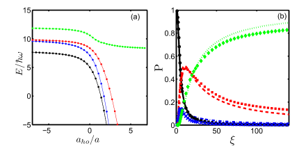
Figure 25: (a) Energy of the most important states amenable to a Landau-Zener description, through the BCS-BEC crossover regime.The black curve corresponds to $\ket{\Psi_{1}}$ which represents the ground state configuration. The blue curve corresponds to $\ket{\Psi_{2}}$ which represents the excited dimer-dimer configuration. The red curve corresponds to $\ket{\Psi_{5}}$ which represents a dimer plus two atoms. The green curve corresponds to $\ket{\Psi_{13}}$ which represents the lowest four-atom configuration. (b) Probability of ending up in a given configuration after the ramp, as a function of the dimensionless speed parameter $\xi$. The symbols correspond to the numerical evolution, while the curves correspond to the Landau-Zener approximation. The colors follow the same convention as Figure (a). Results from Ref. von Stecher and Greene (2007).

The P-matrix analysis also reveals the order in which the transition usually occurs. The order of the peaks reveals the following sequence: the first transition is $1\rightarrow 2$, then $2\rightarrow 5$, then $1\rightarrow 5$, and finally $5\rightarrow 13$. The Landau-Zener prediction for this sequence is

$$p_{1}=(1-T_{1,2})(1-T_{1,5}),$$

$$p_{2}=T_{1,2}(1-T_{2,5}),$$

$$p_{5}=((1-T_{1,2})T_{1,5}+T_{2,5}T_{1,2})(1-T_{5,13}),$$ (86)

$$p_{13}=((1-T_{1,2})T_{1,5}+T_{2,5}T_{1,2})T_{5,13}.$$

Again, the sum of all these probabilities is, by construction, unity. The Landau-Zener parameters obtained from the P-matrix analysis are $\eta_{12}\approx 5.4$, $\eta_{15}\approx 6.6$, $\eta_{25}\approx 2.1$ and $\eta_{5,13}\approx 13.8$. The sequence of Landau-Zener transitions in the model shows good agreement with the numerical results even though many possible transitions have been neglected in the approximate model.

V.7.2 Universal properties

The universal properties of two-component Fermi gases interacting through s-wave collisions has been intensively studied in recent years. Some particularly important research has been carried out concerning the universal properties of four-fermion systems. Here we select two studies that benchmark the universal behavior of four-fermion systems.

The specific point in the strongly-interacting region where the s-wave interaction strength reaches its maximal value, is usually called unitarity. Unitarity is alternatively characterized by a divergent s-wave scattering length, $|a|=\infty$. If inelastic two-body scattering channels are energetically open, the scattering length is complex and it does not diverge all the way to infinity, but the following discussion assumes that such inelastic processes can be neglected. In this situation, if the range of the interaction is much smaller than the typical interparticle distance and if the scattering length is divergent, then no relevant length scale exists that can characterize the interaction. This situation is similar to the noninteracting limit, where the absence of interactions implies, of course, the absence of a length scale that describes the interaction. The absence of a length scale that describes the interaction allows us to extract the functional form of various quantities via dimensional analysis. Furthermore, it allows us to relate quantities at unitarity to those in the noninteracting limit.

Dimensional analysis becomes particularly simple in the hyperspherical framework for a noninteracting or unitary system in free space, where the hyperradius is the only coordinate with dimensions of length. Since the potential curves have units of energy and the only length scale is given by $R$, it follows that $U(R)\propto 1/R^{2}$. This is equivalent to saying that the potential curves at unitarity are proportional to the noninteracting potential curves, i.e.,$U(R)\propto U_{NI}(R)$, since the noninteracting potential curves have the form $1/R^{2}$. The resulting predictions have been derived in Refs. Tan (2004); Werner and Castin (2006).

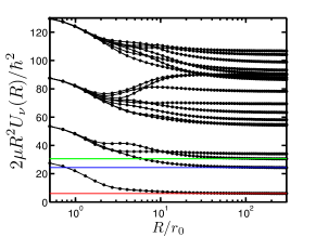
Figure 26: Hyperspherical potential curves at unitarity for the 4-fermion system multiplied by $2\mu R^{2}/\hbar^{2}$. The solid lines represent the predictions extracted from the spectrum obtained with the CG method. The symbols correspond to direct evaluation of the potential curves with the CGHS method. Solid lines correspond to predictions of the large $R$ behavior of the potential curves extracted from the analysis of the excitation spectrum of the four-fermion trapped system.

The four-fermion potential curves calculated at unitarity using CGHS methods allow us to test the premise of universality at the four-body level. Figure 26 presents predictions for the lowest 20 adiabatic potential curves for a Gaussian interaction model potential. At large $R$ the potential curves become proportional to $1/R^{2}$ as predicted by the universal theory. This behavior of the potential curves can be used to understand universal predictions for trapped systems such as the virial theorem and the energy spacing of the trapped spectrum.

The notion of universality extends beyond the unitarity regime and can be applied to any finite scattering length. Recently, Tan was able to derive a series of relations between different observables in two-component Fermi systems Tan (2008a, b, c). These relations were obtained under the premise of universality and are a consequence of the wavefunction behavior when two particles come close together (which is well described by the Bethe-Peierls boundary condition). The universal Tan relations connect the energy, the expectation value of the trapping potential, the pair and momentum distribution functions of two-component Fermi systems through a quantity termed the integrated contact intensity $I(a)$.

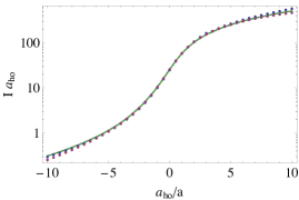
Figure 27: Integrated contact intensity obtained in four different ways: through the analysis of the energy dependence on $a$ (solid curve), virial theorem (dashed curve), momentum distribution (blue symbols), and pair correlation function (red symbols). The solid and dashed curves are essentially indistinguishable on this scale. Figure adapted from Ref. Blume and Daily (2009).

Blume and Daily investigated the Tan relations for a trapped four-fermion systemBlume and Daily (2009). Using the CG method, they extracted the spectrum, the pair correlation function, the momentum distribution and the external potential expectation value for determining $I(a)$ in four different ways. Figure 27 presents a comparison of the different predictions for the contact intensity. The excellent agreement between the different predictions numerically demonstrates the validity of the Tan relations. Furthermore, it quantifies the contact intensity for the four-fermion system, which can serve as a benchmark for further studies.

VI Summary

This review has concentrated on recent developments in the four-body problem, emphasizing those insights that have either used hyperspherical coordinate techniques directly, or else which have benefited indirectly from those insights. The utility of formulating the few-body or even the many-body problem in hyperspherical coordinates was glimpsed early on by some of the pioneers in the field such as DelvesDelves (1959, 1960), Smirnov and ShitikovaSmirnov and Shitikova (1977b), MacekMacek (1968), LinLin (1995), FanoFano (1976), KuppermannKuppermann (1997b), and AquilantiAquilanti and Cavalli (1997). This class of methods has been especially valuable for studying ultracold collisions in recent years, and ultracold applications have been the focus of this overview.

Bosonic four-body systems could not be discussed in much detail in this article, owing to length constraints, but they have provided an important proving ground for many of the methods discussed in the present review. Early ideas on 3-body recombination for three bosons or for three nonidentical fermions that arose first from an adiabatic hyperspherical perspectiveNielsen and Macek (1999); Esry et al. (1999) have since been confirmed and developed further, with many useful new insights from independent theoretical perspectives. The few-body system receiving the most attention over the years has been the three-body problem, both with and without long range Coulombic interactions. The exciting headway represented by that body of literature has had some extensions to handle nontrivial reactive processes for systems with four interacting particles,Greene (2010) and in a handful of studies, for systems with many more particles.Bohn et al. (1998); Blume and Greene (2000); Kim and Zubarev (2000); Kushibe et al. (2004); Sørensen et al. (2002); Rittenhouse et al. (2006); Rittenhouse and Greene (2008)

Numerous questions still remain to be addressed in this field, aiming in the long run towards not only answering questions of universality in the ultracold, but also towards developing systematic ways of handling four-body chemical reaction dynamics at the fully quantum level. A large parameter space also remains to be explored just in the ultracold limit of the four-body problem, such as varying mass ratios for fermionic and for bosonic systems as well as mixed Bose-Fermi systems.

VII Acknowledgments

Many of the results described in this review were developed in close collaboration with Doerte Blume, and we deeply appreciate her contributions and insights. We also thank Brett Esry for numerous informative discussions and for access to some of his results prior to publication. This project was supported by NSF.

Appendix A Hyperangular coordinates

As with Jacobi coordinates, there is no unique way to construct the hyperangles of a system. In this section we construct the hyperangular coordinates used in the four-fermion problem. The choice of hyperangular parameterization has physical meaning. Different parameterizations can be used to describe different correlations within the system. Also, in the case of body-fixed coordinates, hyperspherical coordinates can be used to remove the Euler angles of solid rotation, reducing the dimensionality of the system.

A.1 Delves coordinates

Unfortunately, or possibly fortuitously depending on your view point, there is no unique way to define the hyperangles in a given system. Here we use a simple, standardized method of defining them used by many others Macek (1968); Cavagnero (1986); Bohn et al. (1998); Smirnov and Shitikova (1977a); Rittenhouse et al. (2006); Rittenhouse and Greene (2008) in the form of the so called Delves coordinates Delves (1959, 1960). We will begin by examining a well known example of hyperspherical coordinates, that of normal spherical polar coordinates. Clearly these coordinates can be used to describe the relative motion of 2 particles in 3 dimensions or the position of a single particle in a trap-centered coordinate system, but it can also be used in less obvious ways. For instance, spherical polar angles may be used to describe the relative motion of 4 particles in 1 dimension.

The components of a three dimensional vector, $\bm{r}$, can be written in terms of a radius and two angles as

$$x =r\cos\phi\sin\theta,$$ (87)

$$y =r\sin\phi\sin\theta,$$ (88)

$$z =r\cos\theta.$$ (89)

This parameterization can be represented in a simple tree structure shown in Fig. 28.

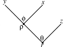
Figure 28: The tree that gives the standard spherical coordinates for a 3 dimensional system is shown.

The end points of the tree represent each component of the vector $\bm{r}$, and each node in the tree is represents an angle. Also associated with each node is a sub radius. For the lowest node the “subradius” is merely the total length of the vector, $r$. For the upper node the subradius is merely the cylindrical radius $\rho=\sqrt{x^{2}+y^{2}}$. Using the tree structure from Fig. 28, a set of rules can be developed for extracting the parameterization of Eqs. (87), (88), and (89). Starting at the bottom node with total radius, $r$, move up through the tree to the desired coordinate. For each move through the tree, if you move to the left (right) from a node multiply by the sine (cosine) of the angle associated with that node. Continue until you reach the Cartesian component.

This procedure can be generalized readily from three to $d$ dimensions. Start by building a tree with $d$ free ends and $d-1$ nodes, associate an angle with each node and follow the above rules. Using the tree structure, starting at the bottom node with total hyperradius, $R$, move up through the tree to the desired coordinate. If you move to the left (right) from a node, multiply by the sine (cosine) of the angle associated with that node. Continue until you have reach the desired Cartesian component. A specific tree for $d$ dimensions is shown in Fig. 29. Following the rules this tree gives the hyperangular representation

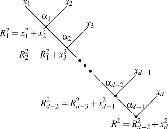
Figure 29: The canonical tree that gives a hyperangular parameterization for a $d$ dimensional system is shown.

$$x_{n} =R\cos\alpha_{n-1}\prod\limits_{j=n}^{d-1}\sin\alpha_{j},$$ (90)

$$0 \leq\alpha_{j}\leq\pi,\text{ }j=2,...,d-1$$

$$0 \leq\alpha_{1}\leq 2\pi$$

where $\cos\alpha_{0}\equiv 1$ and $\prod\limits_{j=d}^{d-1}\sin\alpha_{j}\equiv 1$. This can also be written as

$$\tan\alpha_{n} =\dfrac{\sqrt{\sum_{j=1}^{n}x_{j}^{2}}}{x_{n+1}},$$ (91)

$$n =1,2,3,...,d-1.$$

This hyperspherical tree has been dubbed the canonical tree Avery (1989); Smirnov and Shitikova (1977a) as it is simple to construct and very easy to add more dimensions to.

To avoid double counting, the range that the hyperangles take on is restricted depending on how many free branches are attached to the node corresponding to a given angle. If the node has two free branches, then the angle takes on the full range $0$ to $2\pi$. If the node has one free branch attached, the angle goes from $0$ to $\pi$. If the node has no free branches attached to it, the associated angle goes from $0$ to $\pi/2$. Following these rules for the canonical tree gives the ranges of the angles $\alpha_{i}$,

$$0 \leq\alpha_{1}\leq 2\pi,$$

$$0 \leq\alpha_{i}\leq\pi,i=2,...,d-1.$$

Another slightly more abstract way of considering this construction is to start by breaking the $d$ dimensional space into two subspaces of dimension $d_{1}$ and $d_{2}$, and assuming that these two subspaces are already described by two sets of sub-hyperspherical coordinates, $\left(R_{1},\Omega_{1}\right)$ and $\left(R_{2},\Omega_{2}\right)$. With these assumptions all that remains is to correlate the sub-hyperradii. This is done by following the type of procedure described above using the tree structure shown in Fig. 30,

$$R_{1} =R\sin\alpha,$$ (92)

$$R_{2} =R\cos\alpha,$$

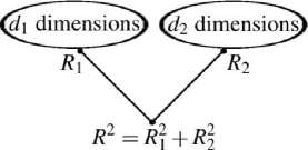
Figure 30: The tree structure used to correlate two subspaces to a single hyperradius.

where $\alpha$ is now the final hyperangle in the system. Using this procedure recursively, one can define the hyperangles in the subspaces until the only remaining subspaces are the individual Cartesian components of the total $d$ dimensional space. The concept of dividing the total space up into subspaces will prove very or the purpose of constructing basis functions.

As a final example of hyperangular parameterizations, we introduce a parameterization for $N$ 3-dimensional vectors $\left\{\bm{\rho}_{i}\right\}_{i=1}^{N}$. One could break each vector up into its individual components and use the canonical parameterization from Eq. (90), but this removes much of the spatial physical intuition that one could bring to bear, such as the individual spatial angular momentum corresponding to each vector. Instead one can use a variation on the canonical tree shown in Fig. 31. On first glance, this tree might seem the same as the canonical tree shown in Fig. 29. In this case, though, the large dot at the end of each branch represents the spherical polar sub-tree of the form shown in Fig. 28 for each vector $\bm{\rho}_{i}$.

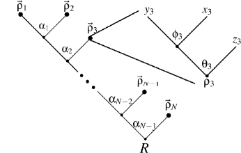
Figure 31: The tree structure used to parameterize the hyperangles for $N$ three dimensional vectors is shown. Note that the dot at the end of each branch in the tree on the left stands for a spherical polar tree.

Using this tree structure and following the rules outlined above, $2N$ of the $3N-1$ hyperangles are given by the normal spherical polar angles for each vector, $\left(\theta_{1},\phi_{1},\theta_{2},\phi_{2},...,\theta_{N},\phi_{N}\right)$. The remaining $N-1$ hyperangles are given by

$$\tan\alpha_{i} =\dfrac{\sqrt{\sum_{j=1}^{i}\rho_{j}^{2}}}{\rho_{i+1}},$$ (93)

$$0 \leq\alpha_{i}\leq\dfrac{\pi}{2},$$

$$i =1,2,3,...,N-1.$$

where $\rho_{i}$ is the length of the $i$th vector. It will be shown in the next section that this parameterization is useful when spatial angular momentum plays a role in the problem of interest. For completeness, following the rules laid out in Appendix A, the hyperangular volume element that results from this parameterization is given by

$$d\Omega=\left(\prod_{i=1}^{N}d\omega_{i}\right)\left(\prod_{j=1}^{N-1}\cos^{2}\alpha_{j}\sin^{3j-1}\alpha_{j}\right)$$

where $\omega_{i}$ is the normal spherical polar differential volume for $\bm{\rho}_{i}$.

The first hyperangular parameterization used here is in the form of Eq. (93) for three 3D vectors. The hyperradius is defined in the same way as in Eq. (114),

$$R^{2}=\sum_{i=1}^{d}x_{i}^{2},$$ (94)

where each $x_{i}$ is a Cartesian component of one of the Jacobi vectors. The hyperspherical trees that will be used for the four fermion problem will of the type in Fig. 31 in which $N$ vectors are described by the spherical polar angles of each vector and a set of hyperangles correlating the lengths of each vector. Specifically, the hyperangles are defined by the tree shown in Fig. 32 combined with the spherical polar angles of each Jacobi vector.

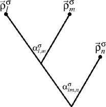
Figure 32: The hyperspherical tree used to parameterize the hyperangular coordinates in the four-fermion problem is shown. See Chapter 2 or Ref. Smirnov and Shitikova (1977a) for details.

Following the rules described above gives the hyperangles,

$$\alpha_{l,m}^{\sigma} =\tan^{-1}\dfrac{\left|\bm{\rho}_{l}^{\sigma}\right|}{\left|\bm{\rho}_{m}^{\sigma}\right|},$$ (95)

$$\alpha_{lm,n}^{\sigma} =\tan^{-1}\dfrac{\sqrt{\left|\bm{\rho}_{l}^{\sigma}\right|^{2}+\left|\bm{\rho}_{m}^{\sigma}\right|^{2}}}{\left|\bm{\rho}_{n}^{\sigma}\right|}.$$

Here the superscript $\sigma=s,i1,i2$ indicates which Jacobi system is being used, while $l,m,n$ indicate the three Jacobi vectors from that system. In principle there are six of these hyperangular coordinate systems that can be constructed from each set of Jacobi vectors giving a total of 18 different hyperangular systems. Fortunately we will not need all of these to tackle the four fermion problem. If one considers two particles, say 1 and 2, the tree defined by Fig. 32 with $\sigma=i1,$ $l=2,m=3$ and $n=1$ can be decomposed into two subtrees. The right branch describes the hyperangular behavior of the dimer alone, while the left branch describes the behavior of the remaining three body system composed of a dimer and two free particles. This type of decomposition will be important for evaluating kinetic energy matrix elements and defining basis functions.

Using the recursive definition of the hyperangular momentum operator in Eq. (117) the total hyperangular momentum operator can be written in terms of the hyperangular coordinates as

$$\Lambda^{2}= \Delta_{1}\left(\alpha_{lm,n}^{\sigma}\right)-\dfrac{1}{\sin^{2}\alpha_{lm,n}^{\sigma}\sin\alpha_{l,m}^{\sigma}\cos\alpha_{l,m}^{\sigma}}\left[\dfrac{\partial}{\partial\alpha_{l,m}^{\sigma}}\right]^{2}\sin\alpha_{l,m}^{\sigma}\cos\alpha_{l,m}^{\sigma}$$ (96)

$$+\dfrac{\hat{l}_{l}^{2}}{\sin^{2}\alpha_{lm,n}^{\sigma}\sin^{2}\alpha_{m,n}^{\sigma}}+\dfrac{\hat{l}_{m}^{2}}{\sin^{2}\alpha_{lm,n}^{\sigma}\cos^{2}\alpha_{m,n}^{\sigma}}+\dfrac{\hat{l}_{n}^{2}}{\cos^{2}\alpha_{lm,n}^{\sigma}},$$

$$\Delta_{1}\left(\alpha_{lm,n}^{\sigma}\right)= \dfrac{-1}{\sin^{2}\alpha_{lm,n}^{\sigma}\cos\alpha_{lm,n}^{\sigma}}\dfrac{1}{\sin\alpha_{lm,n}^{\sigma}}\dfrac{\partial}{\partial\alpha_{lm,n}^{\sigma}}\sin\alpha_{lm,n}^{\sigma}\dfrac{\partial}{\partial\alpha_{lm,n}^{\sigma}}\sin^{2}\alpha_{lm,n}^{\sigma}\cos\alpha_{lm,n}^{\sigma},$$

where $\hat{l}_{l},\hat{l}_{m}$ and $\hat{l}_{n}$ are the normal spatial angular momentum operators for each Jacobi vector. This can also be written directly from Eq. (117) as

$$\Lambda^{2} =\Delta_{1}\left(\alpha_{lm,n}^{\sigma}\right)+\dfrac{\Lambda_{l,m}^{2}}{\sin^{2}\alpha_{lm,n}}+\dfrac{\hat{l}_{n}^{2}}{\cos^{2}\alpha_{lm,n}^{\sigma}},$$ (97)

$$\Lambda_{l,m}^{2} =-\dfrac{1}{\sin\alpha_{l,m}^{\sigma}\cos\alpha_{l,m}^{\sigma}}\left[\dfrac{\partial}{\partial\alpha_{l,m}^{\sigma}}\right]^{2}\sin\alpha_{l,m}^{\sigma}\cos\alpha_{l,m}^{\sigma}+\dfrac{\hat{l}_{l}^{2}}{\sin^{2}\alpha_{m,n}^{\sigma}}+\dfrac{\hat{l}_{m}^{2}}{\cos^{2}\alpha_{m,n}^{\sigma}},$$

where all of the hyperangular behavior above the second node in Fig. 32 is described by a sub-hyperangular momentum, $\Lambda_{lm,n}^{2}$.

Constructing the hyperspherical harmonics for the four-body system is accomplished following the procedure in Section B giving

$$Y_{\left[\lambda\lambda_{l,m}l_{l},l_{m},l_{n}\right]}^{\left(4b\right)}\left(\Omega\right)= N_{l_{l}l_{m}\lambda_{l,m}}^{33}N_{\lambda_{l,m}l_{n},\lambda}^{63}\sin^{\lambda_{l,m}}\left(\alpha_{lm,n}\right)\cos^{l_{n}}\left(\alpha_{lm,n}\right)P_{\left(\lambda-\lambda_{l,m}-l_{n}\right)/2}^{\lambda_{l,m}+5/2,l_{n}+1}\left(\cos 2\alpha_{lm,n}\right)$$ (98)

$$\times N_{l_{l},l_{m}}^{\lambda_{l,m}}\sin^{l_{l}}\left(\alpha_{l,m}\right)\cos^{l_{m}}\left(\alpha_{l,m}\right)P_{\left(\lambda_{l,m}-l_{l}-l_{m}\right)/2}^{l_{l}+1,l_{m}+1}\left(\cos 2\alpha_{l,m}\right)$$

$$\times y_{l_{l}m_{l}}\left(\omega_{l}\right)y_{l_{m}m_{m}}\left(\omega_{m}\right)y_{l_{n}m_{n}}\left(\omega_{n}\right),$$

where $P_{\gamma}^{\alpha,\beta}\left(x\right)$ is a Jacobi polynomial of order $\gamma$, $y_{lm}\left(\omega\right)$ is a normal spherical harmonic with spherical polar solid angle $\omega,$ and $N_{abc}^{de}$ is a normalization constant Smirnov and Shitikova (1977a); Avery (1989):

$$N_{abc}^{de}=\left[\dfrac{\left(2c+d+e-2\right)\Gamma\left(\tfrac{a+b+c+d+e-2}{2}\right)\left(\tfrac{c-a-b}{2}\right)!}{\Gamma\left(\tfrac{c+a-b+d}{2}\right)\Gamma\left(\tfrac{c+b-a+e}{2}\right)}\right]^{1/2}.$$

In Eq. (98) the degeneracy quantum number $\mu$ has been replaced with an explicit tabulation of the hyperangular momentum quantum numbers, i.e. $\lambda\mu\rightarrow\left[\lambda\lambda_{l,m}l_{l},l_{m},l_{n}\right]$. The total four-body hyperspherical harmonics satisfy the eigenvalue equation $\Lambda^{2}Y_{\left[\lambda\lambda_{l,m}l_{l},l_{m},l_{n}\right]}^{\left(4b\right)}\left(\Omega\right)=\lambda\left(\lambda+7\right)Y_{\left[\lambda\lambda_{l,m}l_{l},l_{m},l_{n}\right]}^{\left(4b\right)}\left(\Omega\right)$. The sub-harmonics that are eigenfunctions of $\Lambda_{l,m}^{2}$ can be found as well:

$$Y_{\left[\lambda_{l,m}l_{l},l_{m}\right]}^{\left(3b\right)}\left(\Omega_{l,m}\right)= N_{l_{l},l_{m}\lambda_{l,m}}^{33}\sin^{l_{l}}\left(\alpha_{l,m}\right)\cos^{l_{m}}\left(\alpha_{l,m}\right)P_{\left(\lambda_{l,m}-l_{l}-l_{m}\right)/2}^{l_{l}+1,l_{m}+1}\left(\cos 2\alpha_{l,m}\right)$$ (99)

$$\times y_{l_{l}m_{l}}\left(\omega_{l}\right)y_{l_{m}m_{m}}\left(\omega_{m}\right).$$

Here the superscript, (3b), indicates that this eigenfunction behaves as a 3-body hyperspherical harmonic. For instance if a hyperspherical tree is used with Jacobi vectors defined in the $i1$ interaction coordinate system and $l=1$, $m=3$, and $n=2$, this three-body harmonic describes the free-space behavior of a dimer with two free particles. The three body harmonics obey the eigenvalue equation, $\Lambda_{l,m}^{2}Y_{\left[\lambda_{l,m}l_{l},l_{m}\right]}^{\left(3b\right)}\left(\Omega_{l,m}\right)=\lambda_{l,m}\left(\lambda_{l,m}+4\right)Y_{\left[\lambda_{l,m}l_{l},l_{m}\right]}^{\left(3b\right)}\left(\Omega_{l,m}\right)$. The restrictions on the values of $\lambda$ and $\lambda_{l,m}$ are

$$\lambda_{l,m} =l_{l}+l_{m}+2j,$$ (100)

$$\lambda =\lambda_{l,m}+l_{n}+2k$$

$$=l_{l}+l_{m}+l_{n}+2j+2k,$$

where $j,k=0,1,2,...$. The quantum numbers $l_{l},l_{m}$ and $l_{n}$ are the spatial angular momentum quantum numbers associated with Jacobi vectors $\bm{\rho}_{l}$, $\bm{\rho}_{m}$ and $\bm{\rho_{n}}$ respectively, and each has a z-projection quantum number associated with it which we have suppressed in Eqs. (98) and (99).

A.2 Democratic coordinates

Using Delves coordinates greatly simplifies evaluating hyperangular momentum matrix elements, but it still leaves the 8 dimensional space of hyperangles. I will only be considering systems with total angular momentum $L=0$. Therefore it is convenient to move into a body-fixed coordinate system, as the final wavefunction for the four-body problem will not depend on the Euler angles that produce a solid rotation of the system. Removing the Euler angle dependence is accomplished by transforming into the so-called democratic, or body-fixed coordinates. Four-body democratic coordinates are developed in several references (see Refs. Aquilanti and Cavalli (1997); Kuppermann (1997b); Littlejohn et al. (1999)). In this work we use the parameterization of Aquilanti and Cavalli. For a detailed derivation of the coordinate system see their work in Ref. Aquilanti and Cavalli (1997).

At the heart of democratic coordinates is a rotation from a space fixed frame to a body fixed frame:

$$\bm{\varrho}=\bm{D}^{T}\left(\alpha,\beta,\gamma\right)\bm{\varrho}_{bf}$$ (101)

where $\bm{\varrho}$ is the matrix of Jacobi vectors defined in Eq. (132), $\bm{\varrho}_{bf}$ is the set of body fixed Jacobi coordinates, and $D\left(\alpha,\beta,\gamma\right)$ is an Euler rotation matrix defined in the standard way as

$$\bm{D}=\left[\begin{array}[c]{ccc}\cos\alpha&-\sin\alpha&0\\ \sin\alpha&\cos\alpha&0\\ 0&0&1\end{array}\right]\left[\begin{array}[c]{ccc}\cos\beta&0&\sin\beta\\ 0&1&0\\ -\sin\beta&0&\cos\beta\end{array}\right]\left[\begin{array}[c]{ccc}\cos\gamma&-\sin\gamma&0\\ \sin\gamma&\cos\gamma&0\\ 0&0&1\end{array}\right].$$ (102)

The “$\char 126\relax$” in Eq. (101) indicates a transpose has been taken.

The body-fixed coordinates are defined in a system whose axes are defined by the principle moments of inertia, $I_{1},I_{2}$ and $I_{3}$. In this coordinate system the body-fixed Jacobi coordinates are given by

$$\bm{\varrho}_{bf}=\bm{\Pi}\bm{D}\left(\phi_{1},\phi_{2},\phi_{3}\right),$$ (103)

where $\bm{D}$ is defined in the same way as in Eq. (102) with $\phi_{1},$ $\phi_{2}$ and $\phi_{3}$ replacing $\alpha,$ $\beta,$ and $\gamma$. $\Pi$ is a $3\times 3$ diagonal matrix whose diagonals are given by $\xi_{1},$ $\xi_{2}$ and $\xi_{3}$ which are parameterized by the hyperradius and two hyperangles $\Theta_{1}$ and $\Theta_{2}$:

$$\xi_{1} =\dfrac{R}{\sqrt{3}}\cos\Theta_{1},$$

$$\xi_{2} =\dfrac{R}{\sqrt{3}}\sqrt{3\sin^{2}\Theta_{1}\sin^{2}\Theta_{2}+\cos^{2}\Theta_{1}},$$ (104)

$$\xi_{3} =\dfrac{R}{\sqrt{3}}\sqrt{3\sin^{2}\Theta_{1}\cos^{2}\Theta_{2}+\cos^{2}\Theta_{1}}.$$

To avoid double counting and to allow for different chiralities, $\Theta_{1}$ and $\Theta_{2}$ are restricted to $0\leq\Theta_{1}\leq\pi$ and $0\leq\Theta_{2}\leq\pi/4.$ With this parameterization the moments of inertia are given by

$$\dfrac{I_{1}}{\mu} =\xi_{2}^{2}+\xi_{3}^{2}=\dfrac{R^{2}}{3}\left(2+\sin^{2}\Theta_{1}\right),$$

$$\dfrac{I_{2}}{\mu} =\xi_{1}^{2}+\xi_{3}^{2}=\dfrac{R^{2}}{3}\left(3\sin^{2}\Theta_{1}\cos^{2}\Theta_{2}+2\cos^{2}\Theta_{1}\right),$$ (105)

$$\dfrac{I_{3}}{\mu} =\xi_{1}^{2}+\xi_{2}^{2}=\dfrac{R^{2}}{3}\left(3\sin^{2}\Theta_{1}\sin^{2}\Theta_{2}+2\cos^{2}\Theta_{1}\right).$$

The hyperradius in terms of the principle moments of inertia can be then written as $R^{2}=\xi_{1}^{2}+\xi_{2}^{2}+\xi_{3}^{2}=\left(I_{1}+I_{2}+I_{3}\right)/2\mu.$

With this parameterization, all 8 hyperangles have been defined. The first three are the Euler angles $\left\{\alpha,\beta,\gamma\right\}$, which are external degrees of freedom describing solid rotations of the four body system. The two angles, $\Theta_{1}$ and $\Theta_{2}$, defined in Eq. (104), describe the overall $x,$ $y$ and $z$ extent of the four-body system in the body fixed frame. From Eq. (105), if $\Theta_{1}=0,\pi,$ then the principle moments of inertia are all equal, i.e. $I_{1}=I_{2}=I_{3}$, meaning that the four particles are arranged at the vertices of a regular tetrahedron. When $\Theta_{1}=\pi/2$, Eq. (104) shows that the particles are in a planar configuration. The remaining angles, $\left\{\phi_{1},\phi_{2},\phi_{3}\right\}$, are kinematic rotations within the system, and coalescence points and operations like particle exchange are described in these angles. Broadly speaking, the democratic angles $\Theta_{1}$ and $\Theta_{2}$ can be thought of as correlating the overall $x$, $y$, and $z$ spatial extent of the four-body system in the body-fixed frame, while the kinematic angles $\phi_{1}$, $\phi_{2}$, and $\phi_{3}$ parameterize the internal configuration of the particles.

Since transformations from one Jacobi set to another are merely rotation matrices (sometimes combined with an inversion), the democratic parameterization can always be written in the same form for any given Jacobi coordinate system. For example, the symmetry coordinates [Eq. (123)] can be transformed into the second set interaction coordinates [Eq. (131)] using the kinematic rotation defined by Eq. (141). If the democratic parameterization defined in Eqs. (101) and (103) is used, this transformation reads

$$\bm{\varrho}^{i2} =\bm{D}\left(\alpha,\beta,\gamma\right)\bm{\Pi}\bm{D}^{T}\left(\phi_{1},\phi_{2},\phi_{3}\right)\bm{U}_{s\rightarrow i2},$$

$$=\bm{D}\left(\alpha,\beta,\gamma\right)\bm{\Pi}\bm{D}^{T}\left(\phi_{1}^{\prime},\phi_{2}^{\prime},\phi_{3}^{\prime}\right)$$

where we have used the fact that the product of two rotations in 3D is itself a rotation. From this it is clear that within a given type of Jacobi coordinate (H-type or K-type), all coalescence points are equally well described. This is an important feature as it does not appear in Delves type coordinates, which are strongly dependent on which Jacobi tree is used to define them. For the purposes of this paper, to make symmetrization of the wave function easier, we will always define the body fixed coordinates in terms of the symmetry Jacobi system $\bm{\varrho}^{s}$.

Putting this all together, the body-fixed Jacobi vectors in terms of the internal hyperangles can be defined:

$$\rho_{1x}^{s} =\dfrac{R}{\sqrt{3}}\cos\Theta_{1}\left(\cos\phi_{1}\cos\phi_{2}\cos\phi_{3}-\sin\phi_{1}\sin\phi_{3}\right),$$

$$\rho_{1y}^{s} =\dfrac{R}{\sqrt{3}}\sqrt{\sin^{2}\Theta_{1}\sin^{2}\Theta_{2}+\cos^{2}\Theta_{1}}\left(\sin\phi_{1}\cos\phi_{2}\cos\phi_{3}+\cos\phi_{1}\sin\phi_{3}\right),$$

$$\rho_{1z}^{s} =\dfrac{-R}{\sqrt{3}}\sqrt{\sin^{2}\Theta_{1}\cos^{2}\Theta_{2}+\cos^{2}\Theta_{1}}\sin\phi_{2}\cos\phi_{3},$$ (106)

$$\rho_{2x}^{s} =\dfrac{-R}{\sqrt{3}}\cos\Theta_{1}\left(\cos\phi_{1}\cos\phi_{2}\sin\phi_{3}+\sin\phi_{1}\cos\phi_{3}\right),$$

$$\rho_{2y}^{s} =\dfrac{-R}{\sqrt{3}}\sqrt{\sin^{2}\Theta_{1}\sin^{2}\Theta_{2}+\cos^{2}\Theta_{1}}\left(\sin\phi_{1}\cos\phi_{2}\sin\phi_{3}-\cos\phi_{1}\cos\phi_{3}\right),$$

$$\rho_{2z}^{s} =\dfrac{R}{\sqrt{3}}\sqrt{\sin^{2}\Theta_{1}\cos^{2}\Theta_{2}+\cos^{2}\Theta_{1}}\sin\phi_{2}\sin\phi_{3},$$

$$\rho_{3x}^{s} =\dfrac{R}{\sqrt{3}}\cos\Theta_{1}\cos\phi_{1}\sin\phi_{2},$$

$$\rho_{3y}^{s} =\dfrac{R}{\sqrt{3}}\sqrt{\sin^{2}\Theta_{1}\sin^{2}\Theta_{2}+\cos^{2}\Theta_{1}}\sin\phi_{1}\sin\phi_{2},$$

$$\rho_{3z}^{s} =\dfrac{R}{\sqrt{3}}\sqrt{\sin^{2}\Theta_{1}\cos^{2}\Theta_{2}+\cos^{2}\Theta_{1}}\cos\phi_{2},$$

$$0 \leq\Theta_{1}\leq\pi;0\leq\Theta_{2}\leq\dfrac{\pi}{4},$$

$$0 \leq\phi_{1},\phi_{2},\phi_{3}\leq\pi.$$

The restriction on the range of the internal hyperangles is to avoid double counting configurations and allows for configurations of different chirality .

By moving into democratic coordinates, the dimensionality of the four-body problem can be decreased from 9 to 6, but, as with many simplifications, there is a cost. This cost comes in the form of the differential volume element $d\Omega$ Aquilanti and Cavalli (1997):

$$d\Omega =\left(d\alpha\sin\beta d\beta d\gamma\right)\dfrac{\sqrt{3}\cos^{3}\Theta_{2}\sin^{3}\Theta_{2}\cos 2\Theta_{2}\sin^{9}\Theta_{1}}{\left[\left(\cos^{2}\Theta_{2}+3\sin^{2}\Theta_{1}\cos^{2}\Theta_{2}\right)\left(\cos^{2}\Theta_{2}+3\sin^{2}\Theta_{1}\sin^{2}\Theta_{2}\right)\right]^{1/2}}$$ (107)

$$\times d\Theta_{1}d\Theta_{2}d\phi_{1}\sin\phi_{2}d\phi_{2}d\phi_{3}.$$

The first factor is purely from the Euler angle rotation and will always yield a factor of $8\pi^{2}$ for functions that are independent of $\alpha,$ $\beta$ and $\gamma$.

Another price that is paid using democratic coordinates comes in the form of the hyperangular momentum operator, $\Lambda^{2}$. In terms of the democratic hyperangles, $\Lambda^{2}$ is quite complex and can be found in Ref. Aquilanti and Cavalli (1997):

$$\Lambda^{2}= -\Delta\left(\Theta_{1},\Theta_{2}\right)+2\mu R^{2}\left\{\dfrac{I_{1}}{2\left(I_{2}-I_{3}\right)^{2}}\left(L_{1}^{2}+J_{1}^{2}\right)\right.$$

$$+\dfrac{I_{2}}{2\left(I_{1}-I_{3}\right)^{2}}\left(L_{2}^{2}+J_{2}^{2}\right)+\dfrac{I_{3}}{2\left(I_{1}-I_{2}\right)^{2}}\left(L_{3}^{2}+J_{3}^{2}\right)$$

$$+\dfrac{2\left[I_{1}^{2}-\left(I_{2}-I_{3}\right)^{2}\right]^{1/2}}{\left(I_{2}-I_{3}\right)^{2}}L_{1}J_{1}$$

$$+\dfrac{2\left[I_{2}^{2}-\left(I_{1}-I_{3}\right)^{2}\right]^{1/2}}{\left(I_{1}-I_{3}\right)^{2}}L_{2}J_{2}$$

$$+\left.\dfrac{2\left[I_{3}^{2}-\left(I_{1}-I_{2}\right)^{2}\right]^{1/2}}{\left(I_{1}-I_{2}\right)^{2}}L_{3}J_{3}\right\},$$

where $\bm{J}$ is the total angular momentum operator, and

$$\Delta\left(\Theta_{1},\Theta_{2}\right)= \dfrac{1}{\sin^{7}\Theta_{1}}\dfrac{\partial}{\partial\Theta_{1}}\sin^{7}\Theta_{1}\dfrac{\partial}{\partial\Theta_{1}}+\dfrac{2}{\sin^{2}\Theta_{1}}\left[\dfrac{\partial^{2}}{\partial\Theta_{2}^{2}}+\cot\Theta_{1}\left(\dfrac{4}{\sin^{2}2\Theta_{2}}-1\right)\dfrac{\partial}{\partial\Theta_{1}}\right]$$

$$+\dfrac{4}{\sin^{2}\Theta_{1}}\left\{\dfrac{1}{4\sin 4\Theta_{2}}\dfrac{\partial}{\partial\Theta_{2}}\sin 4\Theta_{2}\dfrac{\partial}{\partial\Theta_{2}}+\dfrac{2}{3}\cot^{2}\Theta_{1}\left[\dfrac{1+3\cos^{2}2\Theta_{2}}{\sin^{2}2\Theta_{2}}\right.\right.$$

$$\times\left.\left.\left(\dfrac{1}{4}\dfrac{\partial^{2}}{\partial\Theta_{2}^{2}}+\dfrac{\cot 2\Theta_{2}}{2}\dfrac{\partial}{\partial\Theta_{2}}\right)-\dfrac{1}{\sin 4\theta_{2}}\dfrac{\partial}{\partial\Theta_{2}}\right]+\cot\Theta_{1}\cot 2\Theta_{2}\dfrac{\partial}{\partial\Theta_{2}}\dfrac{\partial}{\partial\Theta_{2}}\right\}.$$

Terms in $J_{i}^{2}$ are centrifugal contributions, terms in $L_{i}J_{i}$ are Coriolis contributions and terms in $L_{i}^{2}$ are contributions from internal kinematic angular momentum with

$$\bm{L}=i\hbar\left[\begin{array}[c]{ccc}\sin\phi_{1}\cot\phi_{2}&\cos\phi_{1}&-\dfrac{\sin\phi_{1}}{\cos\phi_{2}}\\ \cos\phi_{1}\cot\phi_{2}&-\sin\phi_{1}&-\dfrac{\sin\phi_{1}}{\sin\phi_{2}}\\ 1&0&0\end{array}\right]\left[\begin{array}[c]{c}\dfrac{\partial}{\partial\phi_{1}}\\ \dfrac{\partial}{\partial\phi_{2}}\\ \dfrac{\partial}{\partial\phi_{3}}\end{array}\right].$$

Fortunately, the methods for evaluating matrix elements in what follows will not directly require this form of the hyperangular momentum, but it is included here for completeness.

The final element needed from the democratic coordinates is the inter-particle spacing. The ability to define these will be necessary to describe pairwise interactions and correlations. Using Eqs. (121), (133) and (103),

$$\left|\bm{r}_{12}\right|^{2} =\sqrt{\dfrac{\mu}{\mu_{12}}}\left[\left(\bm{\varrho}_{bf}^{s}\bm{U}_{s\rightarrow i1}\right)^{{\dagger}}\left(\bm{\varrho}_{bf}^{s}\bm{U}_{s\rightarrow i1}\right)\right]_{11},$$ (108)

$$\left|\bm{r}_{13}\right|^{2} =\sqrt{\dfrac{\mu}{\mu_{13}}}\left[\bm{\varrho}_{bf}^{s{\dagger}}\bm{\varrho}_{bf}^{s}\right]_{11},$$ (109)

$$\left|\bm{r}_{14}\right|^{2} =\sqrt{\dfrac{\mu}{\mu_{14}}}\left[\left(\bm{\varrho}_{bf}^{s}\bm{U}_{s\rightarrow i2}\right)^{{\dagger}}\left(\bm{\varrho}_{bf}^{s}\bm{U}_{s\rightarrow i2}\right)\right]_{11},$$ (110)

$$\left|\bm{r}_{23}\right|^{2} =\sqrt{\dfrac{\mu}{\mu_{23}}}\left[\left(\bm{\varrho}_{bf}^{s}\bm{U}_{s\rightarrow i2}\right)^{{\dagger}}\left(\bm{\varrho}_{bf}^{s}\bm{U}_{s\rightarrow i2}\right)\right]_{22},$$ (111)

$$\left|\bm{r}_{24}\right|^{2} =\sqrt{\dfrac{\mu}{\mu_{24}}}\left[\bm{\varrho}_{bf}^{s{\dagger}}\bm{\varrho}_{bf}^{s}\right]_{22},$$ (112)

$$\left|\bm{r}_{34}\right|^{2} =\sqrt{\dfrac{\mu}{\mu_{23}}}\left[\left(\bm{\varrho}_{bf}^{s}\bm{U}_{s\rightarrow i1}\right)^{{\dagger}}\left(\bm{\varrho}_{bf}^{s}\bm{U}_{s\rightarrow i1}\right)\right]_{22},$$ (113)

where $\left[\text{ }\right]_{ij}$ indicates the $ij$th element of a matrix. In this equation, only the body fixed Jacobi coordinates from Eq. (103) are used. This is because the unitary Euler rotation used to rotate into the body fixed frame is the same for all Jacobi coordinates canceling out the $\left\{\alpha,\beta,\gamma\right\}$ dependence in the inter-particle spacings.

Figure 2 shows the surfaces in $\left\{\phi_{1},\phi_{2},\phi_{3}\right\}$ for constant $r_{ij}$ in a planar configuration for $\Theta_{2}=\pi/4,\pi/6,$ and $\pi/12$ for equal mass particles. The $\phi_{1}$ coordinate axis has been transformed to $\phi_{1}-\pi\Theta\left(\phi_{1}-\pi/2\right)$, where $\Theta\left(x\right)$ is the unit step function, to emphasize the symmetry of the surfaces. The red surfaces correspond to the interacting particles in the four-fermion system ($r_{12},r_{14},r_{23}$ and $r_{34}$) while the blue surfaces correspond to the identical fermions ($r_{13}$ and $r_{24}$). The identical particle surfaces surround a coalescence point that must be a Pauli exclusion node in the final four-body wave function. The simple nature of these coalescence points makes clear the reason for choosing to base the democratic coordinates on the symmetry Jacobi vectors. The red surfaces will play an important role in the pairwise interaction as these surfaces outline the valleys of the potential. As the system becomes more linear ($\Theta_{2}$ becomes smaller) it can be seen that the surfaces become broader in the $\phi_{1}$ direction. In fact, when $\Theta_{2}=0$ (in perfectly linear configurations) these surfaces become independent of $\phi_{1}$.

Appendix B Hyperspherical harmonics

Strictly speaking an overview of hyperspherical coordinates is not really needed for this thesis, as there are many excellent existing works on the subject (see for instance Delves (1959, 1960); Avery (1989); Smirnov and Shitikova (1977a); Cavagnero (1986); Bohn et al. (1998)). This section is included here for completeness in order to provide a more complete foundation for the variational basis functions used in this review.

To begin, consider a $d$ dimensional Cartesian space whose coordinate axes are given by $\left\{x_{i}\right\}_{i=1}^{d}$. For the majority of this review these coordinates are considered to be the components of a set of Jacobi vectors or the components of a set of trap centered vectors, but for now we proceed with a more abstract approach. The basic concept of the hyperradius is introduced here as

$$R^{2}=\sum_{i=1}^{d}x_{i}^{2}.$$ (114)

While this definition is used here, often a mass scaling will be inserted. For instance in a trap centered system of equal mass atoms an extra factor of $1/N$, where $N$ is the number of atoms, will be used to simplify the interpretation of the hyperradius. For the purposes of this section, though, this definition will be adequate. With Eq. (114), the $d$ dimensional Laplacian can be rewritten in terms of the hyperradius Avery (1989); Smirnov and Shitikova (1977a):

$$\nabla^{2}=\sum_{i=1}^{d}\dfrac{\partial^{2}}{\partial x_{i}^{2}}=\dfrac{1}{R^{d-1}}\dfrac{\partial}{\partial R}R^{d-1}\dfrac{\partial}{\partial R}-\dfrac{{\Lambda}^{2}}{R^{2}}.$$ (115)

In this equation ${\Lambda}$ is called the hyperangular momentum, or grand angular momentum operator, the square of which is given by

$${\Lambda}^{2} =\sum_{i>j}-\left|\Lambda_{ij}\right|^{2},$$ (116)

$$\Lambda_{ij} =x_{i}\dfrac{\partial}{\partial x_{j}}-x_{j}\dfrac{\partial}{\partial x_{i}}.$$

Already the $d$ dimensional Laplacian has a rather pleasing form reminiscent of its 3D counterpart. In fact if $d$ is taken to $3$, Eq. (115) reduces exactly to the three dimensional Laplacian in spherical coordinates, and ${\Lambda}$ becomes merely the normal spatial angular momentum operator. To proceed from here a way of defining the remaining $d-1$ degrees of freedom in terms of angles is needed.

The hyperangular momentum operator in terms of hyperangular coordinates can be found by using the fact that each subset of Cartesian components is itself a Cartesian vector space. With that in mind, consider the hyperspherical tree given by Fig. 30. By writing the Laplacian for each subspace in terms of the sub-hyperradii $R_{1}$ and $R_{2}$ and the sub-hyperangular momentum operators ${\Lambda}_{1}$ and ${\Lambda}_{2}$ the total hyperangular momentum operator can be extracted Avery (1989). It is

$${\Lambda}^{2} =\dfrac{-1}{\sin^{\left(d_{1}-1\right)/2}\alpha\cos^{\left(d_{2}-1\right)/2}\alpha}\dfrac{\partial^{2}}{\partial\alpha^{2}}\sin^{\left(d_{1}-1\right)/2}\alpha\cos^{\left(d_{2}-1\right)/2}\alpha$$ (117)

$$+\dfrac{{\Lambda}_{1}^{2}+\left(d_{1}-1\right)\left(d_{1}-3\right)/4}{\sin^{2}\alpha}+\dfrac{{\Lambda}_{2}^{2}+\left(d_{2}-1\right)\left(d_{2}-3\right)/4}{\cos^{2}\alpha}-\dfrac{\left(d-1\right)\left(d-3\right)+1}{4}.$$

where $\alpha$ is defined as in Eq. (92) and ${\Lambda}_{i}$ is the sub-hyperangular momentum of the subspace of dimension $d_{i}$. If one of the subspaces corresponds to a single Cartesian component then the sub-hyperangular momentum for that space is zero, i.e. if $d_{i}=1$ then ${\Lambda}_{i}^{2}=0$. To find ${\Lambda}_{1}^{2}$ (${\Lambda}_{2}^{2}$), ones needs only to apply Eq. (117) recursively to each subspace. In this way, there is a sub-hyperangular momentum operator associated with each node in any given hyperspherical tree.

It is useful to be able to diagonalize the hyperangular momentum operator. The eigenfunctions of ${\Lambda}^{2}$ are detailed in several references (See Refs. Macek (1968); Cavagnero (1986); Smirnov and Shitikova (1977a) for example), and the method of constructing them is given in Appendix A. These functions, $Y_{\lambda\mu}\left(\Omega\right)$, are called hyperspherical harmonics. Their eigenvalue equation is

$${\Lambda}^{2}Y_{\lambda\mu}\left(\Omega\right)=\lambda\left(\lambda+d-2\right)Y_{\lambda\mu}\left(\Omega\right),$$ (118)

where $\lambda=0,1,2,...$ is the hyperangular momentum quantum number. The index $\mu$ enumerates the degeneracy for each $\lambda$ and can be thought of as the collection of sub-hyperangular momentum quantum numbers that result from a given tree. Hyperspherical harmonics are also constructed as to diagonalize the sub-hyperangular momenta of each node in a given hyperspherical tree, e.g.

$${\Lambda}_{1}^{2}Y_{\lambda\mu}\left(\Omega\right)=\lambda_{1}\left(\lambda_{1}+d_{1}-2\right)Y_{\lambda\mu}\left(\Omega\right),$$ (119)

where $\lambda_{1}=0,1,2,...$ is the sub-hyperangular momentum quantum number associated with $\Lambda_{1}^{2}$. The total hyperangular momentum quantum number $\lambda$ is limited by the relation

$$\lambda=\left|\lambda_{1}\right|+\left|\lambda_{2}\right|+2n,$$ (120)

where $n$ is a non-negative integer. The absolute values in this case are there to allow for when either $d_{1}$ or $d_{2}$ are $2.$ In this special case the hyperangular momentum quantum number $\lambda_{i}$ associated with the two dimensional subspace can be negative, as with the magnetic quantum number, $m$, in spherical polar coordinates. Equation (120) only applies if both $d_{1}$ and $d_{2}$ are greater than $1$. If, for instance $d_{2}=1$, then the restriction takes on the form

$$\lambda=\left|\lambda_{1}\right|+n.$$

The behavior illustrated in Eq. (119) clearly demonstrates why the parameterization shown in Fig. 31 is useful. Each three dimensional spherical polar subtree will have a spatial angular momentum and z-projection associated with it, e.g.

$$l_{i}^{2}Y_{\lambda\mu}\left(\Omega\right)=l_{i}\left(l_{i}+1\right)Y_{\lambda\mu}\left(\Omega\right),$$

where $l_{i}^{2}$ is the square of the angular momentum operator for the $i$th vector. This property allows for addition of angular momentum in the normal way, through sums over magnetic quantum numbers and Clebsch-Gordan coefficients. Now that the hyperspherical harmonics are defined, it is useful to examine a simple example applying them.

Appendix C Jacobi Coordinate systems and Kinematic rotations

Here we detail the variety of coordinate systems that are used to describe the four-fermion problem in the adiabatic hyperspherical framework and the necessary transformations to describe one set in terms of another. The coordinate systems used here are not only needed to describe correlations between particles, they also allow the system to be reduced in dimensionality by removing the center of mass motion and moving into a body fixed frame. H-type Jacobi coordinates are constructed by considering the separation vector for two two-body subsystems, and the separation vector between the centers of mass of those two subsystems. K-type Jacobi coordinates are constructed in an iterative way by first constructing a three body coordinate set, and then taking the separation vector between the fourth particle and the center of mass of the three particle sub-system.

C.1 Jacobi coordinates: H-trees vs K-trees: fragmentation and symmetry considerations

The first and most obvious symmetry in the four-body Hamiltonian is that of translational symmetry. By describing the system in the center of mass frame, the dimensionality of the system can be reduced from $d=12$ to $d=9$. This is done with the use of Jacobi coordinates. In the interest of brevity, We consider here only those coordinates directly relevant to the four-fermion problem. These coordinates may be broken into two sets, H-type and K-type, shown schematically in Fig. 1.

H-type Jacobi coordinates are constructed by considering the separation vector for two two-body subsystems, and the separation vector between the centers of mass of those two subsystems, i.e.

$$\bm{\rho}_{1}^{H\sigma} =\sqrt{\dfrac{\mu_{ij}}{\mu}}\left(\bm{r}_{i}-\bm{r}_{j}\right),$$

$$\bm{\rho}_{2}^{H\sigma} =\sqrt{\dfrac{\mu_{kl}}{\mu}}\left(\bm{r}_{k}-\bm{r}_{l}\right),$$ (121)

$$\bm{\rho}_{3}^{H\sigma} =\sqrt{\dfrac{\mu_{ij,kl}}{\mu}}\left(\dfrac{m_{i}\bm{r}_{i}+m_{j}\bm{r}_{j}}{m_{i}+m_{j}}-\dfrac{m_{k}\bm{r}_{k}+m_{l}\bm{r}_{l}}{m_{k}+m_{l}}\right),$$

$$\bm{\rho}_{cm} =\dfrac{\left(m_{1}\bm{r}_{1}+m_{2}\bm{r}_{2}+m_{3}\bm{r}_{3}+m_{4}\bm{r}_{4}\right)}{m_{1}+m_{2}+m_{3}+m_{4}},$$

$$\mu_{ij} =\dfrac{m_{i}m_{j}}{m_{i}+m_{j}},\mu_{ij,kl}=\dfrac{\left(m_{i}+m_{j}\right)\left(m_{l}+m_{k}\right)}{m_{1}+m_{2}+m_{3}+m_{4}}.$$

Here the superscript $\sigma$ enumerates the 24 different H-type coordinates that may be obtained through particle permutation, $\bm{\rho}_{cm}$ is the position of center of mass of the four-body system, and $\mu$ is an arbitrary reduced mass for the four-body system. The prefactors in each Jacobi vector, which are given in terms of the various reduced masses in the problem, are chosen to give the so-called mass scaled Jacobi vectors. The kinetic energy in these coordinates can be written as

$$-\sum_{i=1}^{4}\dfrac{\hbar^{2}}{2m_{i}}\nabla_{r_{i}}^{2}=-\dfrac{\hbar^{2}}{2M}\nabla_{\rho_{cm}}^{2}-\dfrac{\hbar^{2}}{2\mu}\sum_{j=1}^{3}\nabla_{\rho_{j}}^{2},$$

where $M$ is the total mass of the four particles. The reduced mass, $\mu$, can be chosen to preserve the differential volume element for the full 3D problem, ensuring that $d^{3}\rho_{1}^{\sigma}d^{3}\rho_{2}^{\sigma}d^{3}\rho_{3}^{\sigma}d^{3}\rho_{cm}=d^{3}r_{1}d^{3}r_{2}d^{3}r_{3}d^{3}r_{4}$:

$$\mu=\left(\dfrac{m_{1}m_{2}m_{3}m_{4}}{m_{1}+m_{2}+m_{3}+m_{4}}\right)^{1/3}.$$

Physically, the H-type coordinates are useful for describing correlations between two particles, for example a two body bound state or a symmetry between two particles, or two separate two-body correlations.

When two particles coalesce [e.g. when $\bm{r}_{i}=\bm{r}_{j}$ in Eq. (121)], the H-type coordinate system reduces to a three body system with two of the four particles acting like a single particle with the combined mass of its constituents:

$$\bm{\rho}_{1}^{H\sigma} =0,$$

$$\bm{\rho}_{2}^{H\sigma} =\sqrt{\dfrac{\mu_{kl}}{\mu}}\left(\bm{r}_{k}-\bm{r}_{l}\right),$$

$$\bm{\rho}_{3}^{H\sigma} =\sqrt{\dfrac{\mu_{ij,kl}}{\mu}}\left(\bm{r}_{i}-\dfrac{m_{k}\bm{r}_{k}+m_{l}\bm{r}_{l}}{m_{k}+m_{l}}\right).$$

Locating these “coalescence points” on the surface of the hypersphere is crucial for accurately describing the interactions between particles, and the coordinate reduction described above will prove useful for the construction of a variational basis set.

K-type Jacobi coordinates are constructed in an iterative way by first constructing a three body coordinate set, and then taking the separation vector between the fourth particle and the center of mass of the three particle sub-system, yielding

$$\bm{\rho}_{1}^{K\sigma} =\sqrt{\dfrac{\mu_{ij}}{\mu}}\left(\bm{r}_{i}-\bm{r}_{j}\right),$$

$$\bm{\rho}_{2}^{K\sigma} =\sqrt{\dfrac{\mu_{ij,k}}{\mu}}\left(\dfrac{m_{i}\bm{r}_{i}+m_{j}\bm{r}_{j}}{m_{i}+m_{j}}-m_{k}\bm{r}_{k}\right),$$ (122)

$$\bm{\rho}_{3}^{K\sigma} =\sqrt{\dfrac{\mu_{ijk,l}}{\mu}}\left(\dfrac{m_{i}\bm{r}_{i}+m_{j}\bm{r}_{j}+m_{k}\bm{r}_{k}}{m_{i}+m_{j}+m_{k}}-m_{l}\bm{r}_{l}\right),$$

$$\bm{\rho}_{cm} =\dfrac{\left(m_{1}\bm{r}_{1}+m_{2}\bm{r}_{2}+m_{3}\bm{r}_{3}+m_{4}\bm{r}_{4}\right)}{m_{1}+m_{2}+m_{3}+m_{4}},$$

$$\mu_{ij} =\dfrac{m_{i}m_{j}}{m_{i}+m_{j}},\mu_{ij,k}=\dfrac{\left(m_{i}+m_{j}\right)m_{k}}{m_{i}+m_{j}+m_{k}},$$

$$\mu_{ijk,l} =\dfrac{\left(m_{i}+m_{j}+m_{k}\right)m_{l}}{m_{1}+m_{2}+m_{3}+m_{4}}.$$

Again $\sigma$ enumerates the 24 different K-type coordinates that result from particle permutations. Examining Fig. 1 shows that K-type Jacobi coordinate systems are useful for describing correlations between three particles within the four particle system. In the four fermion system, there are no weakly bound trimer states meaning that K-type Jacobi coordinates will not be used here, but the methods described in this report can be easily generalized to include these type of states. Unless explicitly stated all Jacobi coordinates from here on will be of the H-type, and for notational simplicity, we will drop the $H$ superscripts.

C.1.1 Coalescence points and permutation symmetry

The proper description of coalescence points is crucial for describing two-body interactions, but they are also important for describing points of symmetry. For instance if two identical fermions are on top of one another it is known that the wave function must vanish at this point owing to the anti-symmetry of fermionic wave functions. Here, we are concerned with four fermions in two different “spin” states. Away from a p-wave resonance, the interactions between identical fermions can be neglected for low energy collisions. This means that there are two types of coalescence points that must be described; two “symmetry” points, when two fermions of the same type are on top of each other, and four “interaction” points, places where two distinguishable fermions interact via an s-wave potential.

It might be tempting at this point to choose a single Jacobi coordinate system and then try to describe the interactions and symmetries in the same coordinates, but this leads to problems. For instance if it is assumed that particles 1 and 3 are spin up and particles 2 and 4 are spin down one might start with coordinates that are simple to anti-symmetrize the system in:

$$\bm{\rho}_{1}^{s} =\sqrt{\dfrac{4^{1/3}}{2}}\left(\bm{r}_{1}-\bm{r}_{3}\right),$$

$$\bm{\rho}_{2}^{s} =\sqrt{\dfrac{4^{1/3}}{2}}\left(\bm{r}_{2}-\bm{r}_{4}\right),$$ (123)

$$\bm{\rho}_{3}^{s} =\sqrt{4^{1/3}}\left(\dfrac{\bm{r}_{1}+\bm{r}_{3}}{2}-\dfrac{\bm{r}_{2}+\bm{r}_{4}}{2}\right),$$

where it has been assumed that all of the particle masses are equal, $m_{1}=m_{2}=m_{3}=m_{4}=m$ leaving $\mu=m/4^{1/3}$. The generalization to distinguishable fermions of different masses is clear. We refer to this Jacobi coordinate system as the symmetry coordinates for fairly obvious reasons. If a permutation of two identical fermions is considered, for instance 1 and 3, the transformation is simple:

$$P_{13}\bm{\rho}_{1}^{s} =-\bm{\rho}_{1}^{s},$$ (124)

$$P_{13}\bm{\rho}_{2}^{s} =\bm{\rho}_{2}^{s},$$ (125)

$$P_{13}\bm{\rho}_{3}^{s} =\bm{\rho}_{3}^{s}.$$ (126)

Similarly for the exchange of particle 2 and 4,

$$P_{24}\bm{\rho}_{1}^{s} =\bm{\rho}_{1}^{s},$$ (127)

$$P_{24}\bm{\rho}_{2}^{s} =-\bm{\rho}_{2}^{s},$$ (128)

$$P_{24}\bm{\rho}_{3}^{s} =\bm{\rho}_{3}^{s}.$$ (129)

The points where two identical fermions coalesce are also simply described by taking either $\bm{\rho}_{1}^{s}\rightarrow 0$ or $\bm{\rho}_{2}^{s}\rightarrow 0$.

The symmetry coordinates are not suited for describing an interaction between two distinguishable fermions, for instance 1 and 2. This interaction occurs around the point $\bm{r}_{1}=\bm{r}_{2}$. In the symmetry coordinates this means that

$$\bm{\rho}_{1}^{s}=\bm{\rho}_{2}^{s}-\sqrt{2}\bm{\rho}_{3}^{s}.$$

This equation describes a 6 dimensional sheet in the 9 dimensional space, something that is not easy to describe directly in any basis set. To get around this problem we introduce two more Jacobi coordinate systems that are useful for describing interactions,

$$\bm{\rho}_{1}^{i1} =\sqrt{\dfrac{4^{1/3}}{2}}\left(\bm{r}_{1}-\bm{r}_{2}\right),$$

$$\bm{\rho}_{2}^{i1} =\sqrt{\dfrac{4^{1/3}}{2}}\left(\bm{r}_{3}-\bm{r}_{4}\right),$$ (130)

$$\bm{\rho}_{3}^{i1} =\sqrt{4^{1/3}}\left(\dfrac{\bm{r}_{1}+\bm{r}_{2}}{2}-\dfrac{\bm{r}_{3}+\bm{r}_{4}}{2}\right),$$

and

$$\bm{\rho}_{1}^{i2} =\sqrt{\dfrac{4^{1/3}}{2}}\left(\bm{r}_{1}-\bm{r}_{4}\right),$$

$$\bm{\rho}_{2}^{i2} =\sqrt{\dfrac{4^{1/3}}{2}}\left(\bm{r}_{3}-\bm{r}_{2}\right),$$ (131)

$$\bm{\rho}_{3}^{i2} =\sqrt{4^{1/3}}\left(\dfrac{\bm{r}_{1}+\bm{r}_{4}}{2}-\dfrac{\bm{r}_{2}+\bm{r}_{3}}{2}\right).$$

The superscript $i1$ and $i2$ in Eqs. (130) and (131) indicate that these Jacobi coordinates are appropriate for interactions between distinguishable fermions. For instance, a coalescence point between particles 1 and 2 is described by $\bm{\rho}_{1}^{i1}\rightarrow 0$. Another benefit of these coordinates is that they are well suited to describing a dimer wavefunction. If particles 2 and 3 are in a weakly bound molecule then the wavefunction for that molecule is only a function of $\bm{\rho}_{2}^{i2}$.

Using combinations of these three coordinate systems, $\bm{\rho}_{j}^{s}$, $\bm{\rho}_{j}^{i1}$ and $\bm{\rho}_{j}^{i2}$, can describe all of the possible two-body correlations of the fermionic system. This assumes that the system in question is that of four equal mass fermions in two internal states with s-wave interactions only. However, the method used is quite general. For instance, K-type coordinates can be chosen to describe the possible three-body correlations that can arise due to Efimov physics in bosonic systems Efimov (1970b, 1973); Braaten and Hammer (2006a).

C.2 Kinematic rotations

Since we use different Jacobi systems to describe different types of correlations, a method of transforming between different sets of coordinates is needed. In the above section, equal mass particles are considered; extension to arbitrary masses is fairly straightforward. To describe the kinematic rotations we keep the masses arbitrary and specify for equal masses later. It is convenient here to deal with transforming all of the Jacobi coordinates at once. Thus the matrices whose columns are made of the Jacobi vectors are used:

$$\bm{\varrho}^{s} =\left\{\bm{\rho}_{1}^{s},\bm{\rho}_{2}^{s},\bm{\rho}_{3}^{s}\right\}$$

$$\bm{\varrho}^{i1} =\left\{\bm{\rho}_{1}^{i1},\bm{\rho}_{2}^{i1},\bm{\rho}_{3}^{i1}\right\}$$ (132)

$$\bm{\varrho}^{i2} =\left\{\bm{\rho}_{1}^{i2},\bm{\rho}_{2}^{i2},\bm{\rho}_{3}^{i2}\right\}.$$

The transformation that takes one coordinate system to another cannot stretch or shrink the differential volume element, and thus it must be a unitary transformation. Further, the transformation cannot mix the Cartesian components of the Jacobi vector, i.e. $\rho_{x}^{i1}$ has no part of $\rho_{y}^{s}$ in it. This means that the transformation will be a unitary matrix that acts from the right, e.g.

$$\bm{\varrho}^{i1}=\bm{\varrho}^{s}\bm{U}_{s\rightarrow i1}.$$ (133)

The matrices that perform these operations are called kinematic rotations Aquilanti and Cavalli (1997); Kuppermann (1997b); Littlejohn et al. (1999), and they will be put to extensive use in the calculations that follow. In truth, transformations between coordinates systems that do not require an inversion should be considered, but the general principle still holds if improper rotations are included. Note that all of the matrix elements must be real, so that the inverse transformation is given merely by the transpose.

We employ a direct “brute force” method of finding these matrices where the system of equations given in Eq. (121) are solved for $\bm{r}_{1}$, $\bm{r}_{2},$ $\bm{r}_{3}$ and $\bm{r}_{4}$ in a given Jacobi system. These normal lab-fixed coordinates can then be inserted into the definition of the Jacobi coordinates that we wish to describe. The kinematic rotation can then be extracted from the resulting relations. Following this procedure gives

$$\bm{U}_{s\rightarrow i1} =\left[\begin{array}[c]{ccc}\tfrac{m_{3}}{m_{1}+m_{3}}\sqrt{\tfrac{\mu_{12}}{\mu_{13}}}&-\tfrac{m_{1}}{m_{1}+m_{3}}\sqrt{\tfrac{\mu_{34}}{\mu_{13}}}&\sqrt{\tfrac{\mu_{13}}{\mu_{12,34}}}\\ -\tfrac{m_{4}}{m_{2}+m_{4}}\sqrt{\tfrac{\mu_{12}}{\mu_{24}}}&\tfrac{m_{2}}{m_{2}+m_{4}}\sqrt{\tfrac{\mu_{34}}{\mu_{24}}}&\sqrt{\tfrac{\mu_{24}}{\mu_{12,34}}}\\ \sqrt{\tfrac{\mu_{12}}{\mu_{13,24}}}&\sqrt{\tfrac{\mu_{34}}{\mu_{13,24}}}&\tfrac{m_{1}m_{4}-m_{2}m_{3}}{\left(m_{1}+m_{2}\right)\left(m_{3}+m_{4}\right)}\sqrt{\tfrac{\mu_{12,34}}{\mu_{13,24}}}\end{array}\right],$$ (137)

$$\bm{U}_{s\rightarrow i2} =\left[\begin{array}[c]{ccc}\tfrac{m_{3}}{m_{1}+m_{3}}\sqrt{\tfrac{\mu_{14}}{\mu_{13}}}&-\tfrac{m_{1}}{m_{1}+m_{3}}\sqrt{\tfrac{\mu_{23}}{\mu_{13}}}&\sqrt{\tfrac{\mu_{13}}{\mu_{12,34}}}\\ \tfrac{m_{4}}{m_{2}+m_{4}}\sqrt{\tfrac{\mu_{14}}{\mu_{24}}}&-\tfrac{m_{2}}{m_{2}+m_{4}}\sqrt{\tfrac{\mu_{23}}{\mu_{24}}}&-\sqrt{\tfrac{\mu_{24}}{\mu_{14,23}}}\\ \sqrt{\tfrac{\mu_{14}}{\mu_{13,24}}}&\sqrt{\tfrac{\mu_{23}}{\mu_{13,24}}}&\tfrac{m_{1}m_{2}-m_{3}m_{4}}{\left(m_{2}+m_{3}\right)\left(m_{1}+m_{4}\right)}\sqrt{\tfrac{\mu_{14,23}}{\mu_{13,24}}}\end{array}\right],$$ (141)

$$\bm{U}_{i1\rightarrow s} =\left[\bm{U}_{s\rightarrow i1}\right]^{T};\text{ }\bm{U}_{i2\rightarrow s}=\left[\bm{U}_{s\rightarrow i2}\right]^{T},$$ (142)

$$\bm{U}_{i1\rightarrow i2} =\bm{U}_{i1\rightarrow s}\bm{U}_{s\rightarrow i2}=\left[\bm{U}_{s\rightarrow i1}\right]^{T}\bm{U}_{s\rightarrow i2};\text{ }\bm{U}_{i2\rightarrow i1}=\left[\bm{U}_{i1\rightarrow i2}\right]^{T}.$$ (143)

The same method can be used to find the kinematic rotations to other Jacobi systems, for instance to K-type coordinates.

Appendix D Implementation of Correlated Gaussian basis set expansion

D.1 Symmetrization of the basis functions and evaluation of the matrix elements

The CG basis functions take the form

$$\Phi_{A}(\bm{x}_{1},\bm{x}_{2},...,\bm{x}_{N})=\mathcal{S}\left\{\exp(-\frac{1}{2}\bm{x}^{T}.\bm{A}.\bm{x})\right\}.$$ (144)

The symmetrization operator $\mathcal{S}$ can be expanded in a set of simple particle permutations,

$$\ket{\mathcal{S}(A)}=\sum^{N_{p}}_{i=1}\mbox{sgn}(P_{i})\ket{P_{i}(A)}.$$ (145)

Here, $N_{p}$ is the number of permutations that characterize the symmetry $\mathcal{S}$. Each of these permutations, $P_{i}$, has a sign associated, $\mbox{sgn}(P_{i})$, and is a given rearrangement of the spatial coordinates

$$P_{i}(\Phi_{A}(\bm{x}_{1},...,\bm{x}_{N})=\Phi_{A}(\bm{x}_{P_{i}(1)},...,\bm{x}_{P_{i}(N)})$$ (146)

The label $i$ characterizes the rearrangement. This rearrangement of the spatial coordinates is equivalent to a rearrangement of the interparticle widths $\{d_{ij}\}$ (or the $\{\alpha_{ij}\}$),

$$P_{k}(\{d_{ij}\})=\{d_{P_{k}(ij)}\}.$$ (147)

Therefore, permutation operations can be easily applied and become transformations of the matrix $A$.

In general the evaluation of the symmetrized matrix elements of an operator $O$ is,

$$\braket{\mathcal{S}(A)}{O}{\mathcal{S}(B)}=\sum^{N_{p}}_{i=1}\sum^{N_{p}}_{i^{\prime}=1}\mbox{sgn}(P_{i})\mbox{sgn}(P_{i^{\prime}})\braket{P_{i^{\prime}}(A)}{O}{P_{i}(A)},$$ (148)

which implies an $N_{p}^{2}$ evaluation of unsymmetrized matrix elements. Fortunately, if $\mathcal{S}(O)=O$ then,

$$\braket{\mathcal{S}(A)}{O}{\mathcal{S}(B)}=N_{p}\braket{A}{O}{\mathcal{S}(B)}=N_{p}\braket{\mathcal{S}(A)}{O}{B}.$$ (149)

This property significantly reduces the numerical demands since the left hand side of Eq.(149) implies $N_{p}^{2}$ permutations, while the right-hand side only implies $N_{p}$ permutations. All operators of the Hamiltonian are invariant under the $\mathcal{S}$, operator and their matrix elements obey Eq.(149).

To obtain density profiles and pair-correlation functions, we use the delta function operator. A single delta function operator in a given coordinate is not invariant under this transformation; for this reason, the computational evaluation is more expensive. Alternatively, we can create a similar operator as a sum of delta functions. If the sum of delta functions reflects the symmetry of the problem, the new operator would be invariant under $\mathcal{S}$.

The permutation operator clearly depends on the symmetry properties of the constituent particles. For identical bosons and fermions,

$$\mathcal{S}=\sum^{N_{p}}_{i=1}\alpha_{i}P_{i},$$ (150)

where $N_{p}=N!$ and $\alpha_{i}=1$ for bosons and $\alpha_{i}=(-1)^{p}$; $p=0,1$ is the parity of the operator $P_{i}$. For two-component systems (boson-boson, fermion-fermion, or a Bose-Fermi mixture),

$$\mathcal{S}=\sum^{N_{p_{1}}}_{i_{1}=1}\sum^{N_{p_{2}}}_{i_{2}=1}\alpha_{i_{1}}\alpha_{i_{2}}P_{i_{1}}P_{i_{2}},$$ (151)

where $N_{p_{1}}=N_{1}!$, $N_{p_{2}}=N_{2}!$, and $N_{1}$ and $N_{2}$ are the number of particles in component 1 and 2, respectively.

The symmetrization operation, if it involves a permutation with a negative sign, can significantly reduce the accuracy of matrix elements. In certain cases, the unsymmetrized matrix elements can be almost identical. Because of the negative sign of the permutation, the symmetrized matrix elements can become a subtraction of very similar numbers. Therefore, accuracy is reduced. These basis functions are usually unphysical, so it is convenient to eliminate them. To do this, we evaluate $|\braket{\mathcal{S}(A)}{\mathcal{S}(A)}|/\max(|\braket{P_{i}(A)}{P_{i}(A)}|)$. If this is a small number, then the accuracy of the matrix elements is reduced. So, in general, we introduce a tolerance of the order of $10^{-3}$ to determine whether to keep or discard the basis functions.

D.2 Evaluation of unsymmetrized basis functions

For convenience, we introduce the following simplify notation,

$$\braket{\bm{x}_{1},\cdots,\bm{x}_{N}}{A}=\exp(-\frac{1}{2}\bm{x}^{T}.\bm{A}.\bm{x}).$$ (152)

As a simple example, consider the overlap matrix element

$$\braket{A}{B}=\int d\bm{x}_{1}..d\bm{x}_{N}\exp(-\frac{1}{2}\bm{x}^{T}.(A+B).\bm{x}).$$ (153)

Since the matrix $A+B$ is real and symmetric, there exists a set of eigenvectors $\bm{y}=\{\bm{y}_{1},...,\bm{y}_{N}\}$ with eigenvalues $\{\beta_{1},...,\beta_{N}\}$ that diagonalize the matrix. In this set of coordinates, Eq. (153) takes the simple form,

$$\braket{A}{B}=(4\pi)^{N}\int_{0}^{\infty}dy_{1}y_{1}^{2}e^{-\beta_{1}y_{1}^{2}/2}...\int_{0}^{\infty}dy_{N}y_{N}^{2}e^{-\beta_{N}y_{N}^{2}/2}=\left(\frac{(2\pi)^{N}}{\det(A+B)}\right)^{3/2}.$$ (154)

Here, we used the product $\beta_{1}.\beta_{2}...\beta_{N}=\det(A+B)$. These basics steps can be followed to evaluate the remaining matrix elements.

To evaluate the kinetic energy, we use the following property,

$$\braket{A}{-\frac{\hbar^{2}}{2m}\nabla^{2}_{\bm{x}_{i}}}{B}=\frac{\hbar^{2}}{2m}\braket{\nabla_{\bm{x}_{i}}A}{\nabla_{\bm{x}_{i}}B}.$$ (155)

This property can be simply proven by applying an integration by parts. Also, it simplifies the matrix element evaluation and provides an expression which is symmetric in $A$ and $B$. Then, the matrix element takes the form,

$$\braket{A}{-\frac{\hbar^{2}}{2m}\sum_{i}^{N}\nabla^{2}_{\bm{x}_{i}}}{B}=\frac{\hbar 2}{2m}3\,\mbox{Tr}((A+B)^{-1}A.B)\braket{A}{B}$$ (156)

Another important matrix element, which is similar to Eq.( 156), is

$$\braket{A}{\bm{x}^{T}C\bm{x}}{B}=\frac{\hbar^{2}}{2m}3\,\mbox{Tr}((A+B)^{-1}C)\braket{A}{B}.$$ (157)

Here, $C$ is an arbitrary matrix. This matrix element is used to calculate the trapping potential energy. In such case, $C=m\omega^{2}I/2$, where $I$ is the identity matrix.

Finally, we calculate the matrix element for a two-body central force:

$$\braket{A}{V(\bm{r}_{i}-\bm{r}_{j})}{B}=\int d^{3}rV(\bm{r})\braket{A}{\delta(b_{ij}^{T}\bm{x}-r)}{B}=G_{c_{ij}}[V]\braket{A}{B},$$ (158)

where $\bm{r}_{i}-\bm{r}_{j}=b_{ij}^{T}\bm{x}$, $c^{{}_{1}}_{ij}=b_{ij}^{T}(A+B)^{-1}b_{ij}$, and $G_{c}[V]$ is the Gaussian transform of the potential

$$G_{c}[V]=\left(\frac{c}{2\pi}\right)^{3/2}\int d^{3}rV(\bm{r})e^{-cr^{2}/2}.$$ (159)

These matrix elements are enough to describe few-body systems.

D.3 Jacobi vectors and CG matrices

Here, we present the construction of the matrices that characterize the basis functions in terms of the widths $d_{ij}$. In the following $\bm{r}=\{\bm{r}_{1},...,\bm{r}_{N}\}$ correspond to Cartesian coordinates, while $\bm{\rho}=\{\bm{\rho}_{1},...,\bm{\rho}_{N-1}\}$ correspond to mass-scaled Jacobi coordinates. First, consider the basis function with the center of mass included

$$\ket{A}=\Psi_{0}(R_{CM})\exp\left(-{\sum_{j\geq i}\frac{(\bm{r}_{1}-\bm{r}_{2})^{2}}{2d_{ij}^{2}}}\right)=\exp(-\frac{1}{2}\bm{r}^{T}.\bm{A}.\bm{r}).$$ (160)

In the equal-mass case for $N$ particles, it is more convenient to simply use Cartesian coordinates. The ground-state–center-of-mass wave function of particles in a harmonic trap takes, conveniently, a Gaussian form $\Psi_{0}(R_{CM})=e^{-NR_{CM}^{2}/2a_{ho}^{2}}$. Thus, $\Psi_{0}(R_{CM})$ can be written as $\Psi_{0}(R_{CM})=e^{-\bm{r}^{T}.M^{CM}.\bm{r}/2}$, where $M^{CM}$ is the center-of-mass matrix whose matrix elements are $M^{CM}_{kl}=1/(Na_{ho}^{2})$ for all $k$ and $l$. Then, for each interparticle distance $r_{ij}$, there exists a matrix $M^{(ij)}$ so that $r_{ij}^{2}=\bm{r}^{T}.M^{(ij)}.\bm{r}$. The matrix elements of the $M^{(ij)}$ matrices are $M^{(ij)}_{ii}=M^{(ij)}_{jj}=1$, $M^{(ij)}_{ij}=M^{(ij)}_{ji}=-1$; the rest are zero, yielding

$$A=M^{CM}+\sum_{j\geq i}\frac{1}{d_{ij}^{2}}M^{(ij)}.$$ (161)

In some cases it is important to include the center-of-mass motion. For example, this allows one to extract single-particle observables such as density profiles.

If the center of mass is not included, then Eq. (161) can be written as,

$$A=\sum_{j>i}\frac{1}{d_{ij}^{2}}M^{(ij)}.$$ (162)

Next, we present the mass-scaled Jacobi vectors (see Fig. 1) and the corresponding form of the matrices $M^{(ij)}$.

Using the H-tree Jacobi coordinates defined in C.1, Eq. (121), the interparticle separation distances can be written:

$$\bm{r}_{1}-\bm{r}_{2}=\bm{\rho}_{1}/d_{1},$$ (163)

$$\bm{r}_{1}-\bm{r}_{3}=\sqrt{\frac{\mu_{3}}{\mu}}\left(\bm{\rho}_{3}+\frac{\mu_{1}d_{3}}{m_{1}d_{1}}\bm{\rho}_{1}-\frac{\mu_{2}d_{3}}{m_{3}d_{2}}\bm{\rho}_{2}\right),$$ (164)

$$\bm{r}_{1}-\bm{r}_{4}=\sqrt{\frac{\mu_{3}}{\mu}}\left(\bm{\rho}_{3}+\frac{\mu_{1}d_{3}}{m_{1}d_{1}}\bm{\rho}_{1}+\frac{\mu_{2}d_{3}}{m_{4}d_{2}}\bm{\rho}_{2}\right),$$ (165)

$$\bm{r}_{2}-\bm{r}_{3}=\sqrt{\frac{\mu_{3}}{\mu}}\left(\bm{\rho}_{3}-\frac{\mu_{1}d_{3}}{m_{2}d_{1}}\bm{\rho}_{1}+\frac{\mu_{2}d_{3}}{m_{3}d_{2}}\bm{\rho}_{2}\right),$$ (166)

$$\bm{r}_{2}-\bm{r}_{4}=\sqrt{\frac{\mu_{3}}{\mu}}\left(\bm{\rho}_{3}-\frac{\mu_{1}d_{3}}{m_{2}d_{1}}\bm{\rho}_{1}+\frac{\mu_{2}d_{3}}{m_{4}d_{2}}\bm{\rho}_{2}\right),$$ (167)

$$\bm{r}_{3}-\bm{r}_{4}=\bm{\rho}_{2}/d_{2}.$$ (168)

For both the $N=3$ and $N=4$ systems, the interparticle distances can be written in terms of the Jacobi vectors

$$\bm{r}_{i}-\bm{r}_{j}=\sum_{k}c_{k}^{(ij)}\bm{\rho}_{k}.$$ (169)

Now we can write the matrices $M^{(ij)}$ in these Jacobi vectors that describe an interparticle distance. The matrix elements of these matrices are simply $M^{(ij)}_{kl}=c_{k}^{(ij)}c_{l}^{(ij)}$.

D.4 Selection of the basis set

There are different strategies for selecting a basis set. If the numbers of dimensions of the system we are studying is not that large, then we can try to generate a large basis set that is complete enough to describe several eigenstates at different interaction strengths.

The Gaussian widths $d_{ij}$ are selected randomly and cover a range of values from $d_{0}$ to the trap length $a_{ho}$. Specifically, the $d_{ij}$ are selected randomly using a Gaussian distribution of range 1 and then scaled to three different distances: $d_{0}$, an intermediate distance $\sqrt{d_{0}a_{ho}}$, and $a_{ho}$. These three distances are fixed once the interparticle potential range $d_{0}$ is fixed.

The basis set selection depends on the correlation we want to describe. So, the selection process changes depending whether the particles are bosons or fermions. For fermions, when there is no trimer formation, basis functions with more than two particles close together are not important.

For example, the algorithm for the selection of the basis functions for a two-component four-fermion system divides the basis into three parts: the first subbasis generates $d_{ij}$, which are all of the order of $a_{ho}$; they are useful for describing weakly interacting states. The second subbasis generates two $d_{ij}$ of the order of $d_{0}$ or $\sqrt{d_{0}a_{ho}}$ and the rest of the order of $a_{ho}$; they are useful to describe dimer-dimer states. The third subbasis has one $d_{ij}$ of the order of $d_{0}$ or $\sqrt{d_{0}a_{ho}}$ and the rest of the order of $a_{ho}$. They are useful to describe dimer–two-free-atom states.

D.5 Controlling Linear dependence

A large basis set is usually needed to describe several eigenstates in a wide range of interactions. Since the basis set is over complete and the basis functions are chosen semi-randomly, the resulting basis can have linear dependence problems. In our implementation we eliminate the linear dependence by reducing the size of basis set.

To do this, we first diagonalize the overlap matrix and then eliminate the eigenstates with negative or low eigenvalues. The remaining eigenstates form an orthonormal basis set. Finally, we transform the Hamiltonian to the new orthonormal basis set.

The threshold for the elimination can be selected automatically taking into account the lowest eigenvalue. If the lowest eigenvalue $O_{1}$ is small and positive, the tolerance can be selected as, for example, $10^{3}O_{1}$. If $O_{1}$ is negative and the magnitude is large, then the basis set has a lot of linear dependence, and it is more convenient to change the initial basis set.

D.6 Stochastical variational method

The SVM has been developed in the context of nuclear physics to solve few-body problems Varga and Suzuki (1995, 1996, 1997). It allows a systematically improvement of the basis set. A detailed discussion of the implementation of the SVM will not be presented here but can be found in Refs. Sørensen (2005); Suzuki and Varga (1998). In the following, we present the main concepts of the SVM.

The SVM is based on the variational nature of the spectrum obtained by a basis set expansion. Consider a basis set of size $D$ with eigenvalues $\{\epsilon_{1},...,\epsilon_{D}\}$, if we add a new basis function then the new eigenvalues $\{\lambda_{1},...,\lambda_{D+1}\}$ obey $\lambda_{1}\leq\epsilon_{1}\leq\lambda_{2}...\epsilon_{D}\leq\lambda_{D+1}$. Here, we assume that both set of eigenvalues are arranged in increasing order. Thus, by adding a new basis, all the $D$ eigenvalues should decrease or remain the same. Therefore, the lower the new eigenvalues are the better the improvement of the basis set. Thus we can test the utility of the added basis function by considering the improvement in the eigenvalues.

In most cases, we are not interested in improving the complete spectrum. To select which states or energies we want to improve, we can construct an appropriate minimization function. This function would depend only on the energies we want to improve and is minimized by the SVM.

In order to optimize the basis set, the SVM utilizes a trial an error procedure. Starting from an initial basis set of size $D$, several basis functions are selected stochastically and added, one at a time, to the basis set. For each $D+1$ basis set, the new eigenvalues are evaluated. The basis function that produces the best improvement of the selected energies is kept while the remaining basis functions are discarded. The initial basis function is then increased by one and the trial an error procedure is repeated.

If this procedure is continued indefinitely the size of the basis set has become large and the calculations become forbiddingly slow. Therefore, it is convenient to increase the basis up to a reasonable size and then continue the optimization process without increasing the basis size. This optimization can be carried out by a refinement process. Instead of adding a new basis function, we test the importance of the basis functions of the basis set. The trial and error procedure is then applied to each of the functions of the basis set.

For the SVM procedure to be efficient, the evaluation of both the matrix elements and the eigenvalues need to be fast and accurate. It is particularly important to obtain very accurate matrix elements because the improvement due to a single basis function is usually very small and can only be evaluated reliably if the matrix element are very accurate. The matrix element evaluation in the CG and CGHS is both fast and accurate making these methods particularly suitable for SVM optimization.

Also, the evaluation of the eigenvalues can be significantly speeded up in the trial and error procedure. The basis functions are added or replaced one by one which allowing us to reduce the evaluation of the eigenvalues to a root finding procedure. This root finding procedure is much faster than any diagonalization procedure.

The SVM automatically takes care of the selection of the basis function. Also, it tries to avoid linear dependence in the basis set by constraining the normalized overlap between any two basis function, i.e., $O_{12}/\sqrt{O_{11}O_{22}}$, to be below some tolerance $O_{max}$. The tolerance $O_{max}$ is usually selected between 0.95 and 0.99. For example, the size of the basis set of $N=3$ and $4$ can be increased up to 700 and 8000 respectively without introducing significant linear dependence.

Appendix E Dimer-Dimer Relaxation Rates

In this appendix I present the derivation of the dimer-dimer relaxation rate used in Section 6.5. This process occurs when the two dimers collide causing at least one of the dimers to relax to a deeply bound state. The difference of the binding energies is then releases as kinetic energy. This process can be pictured in the hyperspherical picture as an infinite series of very closely spaced crossings between the dimer-dimer channel and channels consisting of a deeply bound dimer and two free particles. This near continuum of crossings is shown schematically in Fig. 33(a).

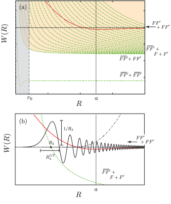
Figure 33: (a) A schematic of the channels involved involved inthe dimer-dimer relazaxtion process is shown. The dimer-dimer potential (red curve) goes through an inifinite number of crossing with deeply bound states (green dashed curves). (b) The hyperradial behavior of the outgoing wavefunction is shown.

Using Fermi’s golden rule between the initial dimer-dimer state and the final states gives

$$V_{rel}^{dd}\propto\sum_{\lambda}\left|\left\langle\Psi_{dd}\left(R;\Omega\right)\left|V\left(R,\Omega\right)\right|\Psi_{\lambda}\left(R,\Omega\right)\right\rangle\right|^{2},$$ (170)

where $\Psi_{dd}\left(R;\Omega\right)$ is the dimer-dimer wavefunction, $V\left(R,\Omega\right)$ is the interaction potential and $\Psi_{k}$ is the $\lambda$th deeply bound dimer state. I now will assume that the dimer-dimer wavefunction is approximated by

$$\Psi_{dd}\left(R;\Omega\right)\approx F_{dd}\left(R\right)\Phi_{dd}\left(R;\Omega\right),$$ (171)

where $\Phi_{dd}\left(R;\Omega\right)$ is the dimer-dimer hyperangular channel function and $F_{dd}\left(R\right)$ is the hyperradial wavefunction resulting from the single channel approximation. I further assume that the outgoing deeply bound dimer wavefunction can be written as

$$\Psi_{k}\left(R,\Omega\right)\approx\psi\left(r_{12}\right)\theta_{\lambda}\left(\vec{r}_{34},\vec{r}_{12,34}\right)$$ (172)

where $\psi\left(r_{12}\right)$ is the wavefunction for an s-wave deeply bound dimer and $\theta_{\lambda}\left(\vec{r}_{34},\vec{r}_{12,34}\right)$ is the free space behavior of the resulting three particle system.

Examining one of the terms from the sum in Eq. (170) with a single two-body interaction gives

$$V_{rel}^{dd\left(\lambda\right)}\propto\left|\int F_{dd}\left(R\right)\Phi_{dd}\left(R;\Omega\right)V_{23}\left(r_{23}\right)\psi\left(r_{12}\right)\theta_{\lambda}\left(\vec{r}_{34},\vec{r}_{12,34}\right)dRd\Omega\right|^{2},$$ (173)

where $V_{rel}^{dd\left(k\right)}$ is the contribution to the relaxation rate by the $\lambda$th term in Eq. (170). The first thing to notice is in this is that the factor $V_{23}\left(r_{23}\right)\psi\left(r_{12}\right)$ is non-zero only when particles $1,2,$ and $3$ are in close proximity, and when particles $1,2,$ and $3$ are in close proximity the remaining degrees of freedom are simplified as well,

$$\vec{r}_{34}\approx C\vec{r}_{12,34}.$$ (174)

This means that the wavefunction $\theta\left(\vec{r}_{34},\vec{r}_{12,34}\right)$ can be rewritten as

$$\theta_{\lambda}\left(\vec{r}_{34},\vec{r}_{12,34}\right)\approx G_{\lambda}\left(R\right)f_{\lambda}\left(\Omega\right),$$ (175)

where $G_{\lambda}$ and $f_{\lambda}$ are the hyperradial and hyperangular behavior associated with the $\lambda$th outgoing channel. A further simplification can be made by realizing that $f_{\lambda}\left(\Omega\right)$ must be independent of $\Omega$ when particles $1,2,$ and $3$ are in close proximity because the total wavefunction must have zero spatial angular momentum. Rewriting (173) with these simplifications yields

$$V_{rel}^{dd\left(\lambda\right)}\propto\left|\int F_{dd}\left(R\right)G_{k}\left(R\right)\int\Phi_{dd}\left(R;\Omega\right)V_{23}\left(r_{23}\right)\psi\left(r_{12}\right)d\Omega dR\right|^{2}.$$ (176)

The hyperangular integral is approximated by the probability that three-particles are close to each other in the dimer-dimer channel function.

And example of $G_{\lambda}$ is shown in Fig. 33(b). Away from the classical turning point $G_{\lambda}$ oscillates very rapidly. This fast oscillation will generally cancel out meaning the main contribution to the hyperradial integral is from the region near the classical turning point $R_{\lambda}.$ Putting this all together yields

$$V_{rel}^{dd}\propto\sum_{\lambda}\dfrac{\left|F_{dd}\left(R_{\lambda}\right)\right|^{2}}{R_{\lambda}}\mathcal{F}\left(R_{\lambda}\right),$$ (177)

where $\mathcal{F}\left(R_{\lambda}\right)$ is the probability that three particles are in close proximity in the dimer-dimer channel function. The final step in this derivation is to turn the sum over $\lambda$ into an integral over $R_{\lambda}$,

$$V_{rel}^{dd}\propto\int\rho\left(R_{\lambda}\right)\dfrac{\left|F_{dd}\left(R_{\lambda}\right)\right|^{2}}{R_{\lambda}}\mathcal{F}\left(R_{\lambda}\right)dR_{\lambda}$$ (178)

where $\rho\left(R_{\lambda}\right)$ is the, nearly constant, density of states. This is possible due to the near-continuum nature of the outgoing states. By inserting the WKB approximation wavefunction for $F_{dd}\left(R\right)$, the result of Eq. (68) is obtained, i.e.

$$V_{rel}^{dd}\propto\int\rho\left(R\right)\dfrac{P_{WKB}\left(R_{\lambda}\right)}{\kappa\left(R\right)R}\mathcal{F}\left(R\right)dR.$$ (179)

References

- Hu and Schatz (2006) W. Hu and G. C. Schatz, J. Chem. Phys. 125, 132301 (2006).
- Clary (1998) D. C. Clary, Science 279, 1879 (1998).
- Wigner (1933) E. Wigner, Phys. Rev. 43, 252 (1933).
- Bethe and Bacher (1936) H. A. Bethe and R. F. Bacher, Rev. Mod. Phys. 8, 82 (1936).
- Lin (1986a) C. D. Lin, Adv. At. Molec. Phys. 22, 77 (1986a).
- Fano (1983) U. Fano, Rep. Prog. Phys. 46, 97 (1983).
- Solov’ev and Tolstikhin (2001) E. A. Solov’ev and O. I. Tolstikhin, J. Phys. B 34, L439 (2001).
- Tolstikhin et al. (1996) O. I. Tolstikhin, S. Watanabe, and M. Matsuzawa, J. Phys. B 29, L389 (1996).
- Archer et al. (1990) B. J. Archer, G. A. Parker, and R. T. Pack, Phys. Rev. A 41, 1303 (1990).
- Esry et al. (1999) B. D. Esry, C. H. Greene, and J. P. Burke Jr, Phys. Rev. Lett. 83, 1751 (1999).
- Nielsen and Macek (1999) E. Nielsen and J. H. Macek, Phys. Rev. Lett. 83, 1566 (1999).
- Braaten and Hammer (2006a) E. Braaten and H.-W. Hammer, Phys. Rep. 428, 259 (2006a).
- Parker et al. (2002) G. A. Parker, R. B. Walker, B. K. Kendrick, and R. T. Pack, J. Chem. Phys. 117, 6083 (2002).
- Quéméner et al. (2007) G. Quéméner, J.-M. Launay, and P. Honvault, Phys. Rev. A 75, 050701 (2007).
- Honvault and Launay (2001) P. Honvault and J.-M. Launay, J. Chem. Phys. 114, 1057 (2001).
- Yang et al. (1995) X. Z. Yang, J. H. Xi, C. G. Bao, and C. D. Lin, Phys. Rev. A 52, 2029 (1995).
- Yang et al. (1996) X. Z. Yang, C. G. Bao, and C. D. Lin, Phys. Rev. Lett. 76, 3096 (1996).
- Morishita et al. (1997) T. Morishita, O. I. Tolstikhin, S. Watanabe, and M. Matsuzawa, Phys. Rev. A 56, 3559 (1997).
- Morishita and Lin (1998) T. Morishita and C. D. Lin, Phys. Rev. A 57, 4268 (1998).
- Morishita and Lin (1999) T. Morishita and C. D. Lin, Phys. Rev. A 59, 1835 (1999).
- D’Incao (2003) J. P. D’Incao, Phys. Rev. A 67, 024501 (2003).
- Morishita and Lin (2003) T. Morishita and C. D. Lin, Phys. Rev. A 67, 022511 (2003).
- Madsen (2003) L. B. Madsen, J. Phys. B 36, R223 (2003).
- Brooks and Clary (1990) A. N. Brooks and D. C. Clary, J. Chem. Phys. 92, 4178 (1990).
- Clary (1991) D. C. Clary, J. Chem. Phys. 95, 7298 (1991).
- Clary (1992) D. C. Clary, J. Chem. Phys. 96, 3656 (1992).
- Quéméner and Balakrishnan (2009) G. Quéméner and N. Balakrishnan, J. Chem. Phys. 130, 114303 (2009).
- Zhang and Light (1997) D. H. Zhang and J. C. Light, J. Chem. Phys. 106, 551 (1997).
- Vijande et al. (2009) J. Vijande, A. Valcarce, J. M. Richard, and N. Barnea, Few-Body Syst. 45, 99 (2009).
- Thomas (1935) L. H. Thomas, Phys. Rev. 47, 903 (1935).
- Delves (1959) L. M. Delves, Nucl. Phys 9, 391 (1959).
- Delves (1960) L. M. Delves, Nucl. Phys. 20, 275 (1960).
- Efimov (1970a) V. Efimov, Phys. Lett. B 33, 563 (1970a).
- Efimov (1971) V. Efimov, Sov. J. Nucl. Phys 12, 589 (1971).
- Fock (1958) V. Fock, K. Norske Vidensk. Selsk. Forhandl. 31, 138 (1958).
- Klar (1985) H. Klar, J. Phys. B 18, L475 (1985).
- Forrey (2004) R. C. Forrey, Phys. Rev. A 69, 022504 (2004).
- Macek (1968) J. H. Macek, J. Phys. B 1, 831 (1968).
- Fano (1981) U. Fano, Phys. Rev. A 24, 2402 (1981).
- Lin (1995) C. D. Lin, Phys. Rep. 257, 1 (1995).
- Domke et al. (1991) M. Domke, C. Xue, A. Puschmann, T. Mandel, E. Hudson, D. Shirley, G. Kaindl, C. H. Greene, H. R. Sadeghpour, and H. Petersen, Phys. Rev. Lett. 66, 1306 (1991).
- Sadeghpour and Greene (1990) H. R. Sadeghpour and C. H. Greene, Phys. Rev. Lett. 65, 313 (1990).
- Klar and Klar (1978) H. Klar and M. Klar, Phys. Rev. A 17, 1007 (1978).
- Jonsell et al. (2002) S. Jonsell, H. Heiselberg, and C. J. Pethick, Phys. Rev. Lett. 89, 250401 (2002).
- Bondi et al. (1983) D. K. Bondi, J. N. L. Connor, J. Manz, and J. Romelt, Mol. Phys. 50, 467 (1983).
- Chuluunbaatar et al. (2008) O. Chuluunbaatar, A. A. Gusev, S. I. Vinitsky, and A. G. Abrashkevich, Comp. Phys. Comm. 179, 685 (2008).
- Nikitin (1970) E. E. Nikitin, Teoriya Elementarnykh Atomnomolekulyarnykh Protsessov Ì Gazakh (Theory of Elementary Atomómolecule Processes in Gases) (Izd. Khimiya, 1970).
- Clark and Greene (1980) C. W. Clark and C. H. Greene, Phys. Rev. A 21, 1786 (1980).
- Greene and Clark (1984) C. H. Greene and C. W. Clark, Phys. Rev. A 30, 2161 (1984).
- Kokoouline et al. (2001) V. Kokoouline, C. H. Greene, and B. D. Esry, Nature 412, 891 (2001).
- Kokoouline and Greene (2003) V. Kokoouline and C. H. Greene, Phys. Rev. A 68, 012703 (2003).
- dos Santos et al. (2007) S. F. dos Santos, V. Kokoouline, and C. H. Greene, J. Chem. Phys. 127, 124309 (2007).
- Kuppermann (1997a) A. Kuppermann, Journal of Physical Chemistry A 101 (1997a).
- Lepetit et al. (2006) B. Lepetit, D. Wang, and A. Kuppermann, J. Chem. Phys. 125 (2006).
- Aquilanti and Cavalli (1997) V. Aquilanti and S. Cavalli, J. Chem. Soc., Faraday Transactions 93, 801 (1997).
- Weiner et al. (1999) J. Weiner, V. S. Bagnato, S. Zilio, and P. S. Julienne, Rev. Mod. Phys. 71, 1 (1999).
- Gao et al. (2005) B. Gao, E. Tiesinga, C. J. Williams, and P. S. Julienne, Phys. Rev. A 72, 042719 (2005).
- Gao (2008) B. Gao, Phys. Rev. A 78, 012702 (2008).
- Raoult and Mies (2004) M. Raoult and F. H. Mies, Phys. Rev. A 70, 012710 (2004).
- Mies and Raoult (2000) F. H. Mies and M. Raoult, Phys. Rev. A 62, 012708 (2000).
- Burke Jr (1999) J. P. Burke Jr, Ph.D. thesis, University of Colorado (1999).
- Burke et al. (1998) J. P. Burke, C. H. Greene, and J. L. Bohn, Phys. Rev. Lett. 81, 3355 (1998).
- Zaccanti et al. (2009) M. Zaccanti, B. Deissler, C. D’Errico, M. Fattori, M. Jona-Lasinio, S. M¸ller, G. Roati, M. Inguscio, and G. Modugno, Nat. Phys. 5, 586 (2009).
- Kraemer et al. (2006) T. Kraemer, M. Mark, P. Waldburger, J. G. Danzl, C. Chin, B. Engeser, A. D. Lange, K. Pilch, A. Jaakkola, H. C. Naegerl, et al., Nature 440, 315 (2006).
- Braaten and Hammer (2006b) E. Braaten and H. W. Hammer, Phys. Rep. 428, 259 (2006b).
- Moroz et al. (2009) S. Moroz, S. Floerchinger, R. Schmidt, and C. Wetterich, Phys. Rev. A 79, 042705 (2009).
- Shepard (2007) J. R. Shepard, Phys. Rev. A 75, 062713 (2007).
- Massignan and Stoof (2008) P. Massignan and H. T. C. Stoof, Phys. Rev. A 78, 030701 (2008).
- Lee et al. (2007) M. D. Lee, T. Köhler, and P. S. Julienne, Phys. Rev. A. 76, 012720 (2007).
- Gogolin et al. (2008) A. O. Gogolin, C. Mora, and R. Egger, Phys. Rev. Lett. 100, 140404 (2008).
- Feenberg (1936) E. Feenberg, Phys. Rev. 49, 328 (1936).
- Fedichev et al. (1996) P. O. Fedichev, M. W. Reynolds, and G. V. Shlyapnikov, Phys. Rev. Lett. 77, 2921 (1996).
- Regal et al. (2004) C. A. Regal, M. Greiner, and D. S. Jin, Phys. Rev. Lett. 92, 083201 (2004).
- Bourdel et al. (2004) T. Bourdel, L. Khaykovich, J. Cubizolles, J. Zhang, F. Chevy, M. Teichmann, L. Tarruell, S. Kokkelmans, and C. Salomon, Phys. Rev. Lett. 93, 50401 (2004).
- D’Incao et al. (2009a) J. P. D’Incao, S. T. Rittenhouse, N. P. Mehta, and C. H. Greene, Phys. Rev. A 79, 030501 (2009a).
- Hammer and Platter (2007) H.-W. Hammer and L. Platter, Eur. Phys. J. A 32, 113 (2007).
- von Stecher et al. (2009) J. von Stecher, J. P. D’Incao, and C. H. Greene, Nat. Phys. 5, 417 (2009).
- von Stecher and Greene (2009a) J. von Stecher and C. H. Greene, Phys. Rev. A 80, 022504 (2009a).
- Ferlaino et al. (2009) F. Ferlaino, S. Knoop, M. Berninger, W. Harm, J. P. D’Incao, H.-C. Nägerl, and R. Grimm, Phys. Rev. Lett. 102, 140401 (2009).
- Mehta et al. (2009) N. P. Mehta, S. T. Rittenhouse, J. P. D’Incao, J. von Stecher, and C. H. Greene, Phys. Rev. Lett. 103, 153201 (2009).
- D’Incao et al. (2009b) J. P. D’Incao, J. von Stecher, and C. H. Greene, Phys. Rev. Lett. 103, 033004 (2009b).
- Deltuva (2010) A. Deltuva, Phys. Rev. A 82, 040701 (2010).
- Wang and Esry (2009) Y. Wang and B. D. Esry, Phys. Rev. Lett 102, 133201 (2009).
- Zhu et al. (2001) C. Zhu, Y. Teranishi, and H. Nakamura, in Adv. Chem. Phys. (John Wiley & Sons Inc, 2001), vol. 117 of Advances in Chemical Physics, pp. 127–233.
- Child (1991) M. S. Child, Semiclassical Methods with Molecular Applications (Clarendon Press, Oxford, 1991).
- Miller and George (1972) W. H. Miller and T. F. George, J. Chem. Phys. 56, 5668 (1972).
- Chin et al. (2010) C. Chin, R. Grimm, P. S. Julienne, and E. Tiesinga, Rev. Mod. Phys. 82, 1225 (2010).
- Esry et al. (2001) B. D. Esry, C. H. Greene, and H. Suno, Phys. Rev. A 65, 010705(R) (2001).
- D’Incao and Esry (2005) J. P. D’Incao and B. D. Esry, Phys. Rev. Lett. 94, 213201 (2005).
- D’Incao and Esry (2009) J. P. D’Incao and B. D. Esry, Phys. Rev. Lett. 103, 083202 (2009).
- Avery (1989) J. Avery, Hyperspherical Harmonics: Applications in Quantum Theory (Kluwer Academic Publishers, Norwell, MA, 1989).
- Berry (1966) M. V. Berry, Proc. Phys. Soc. 88, 285 (1966).
- Langer (1937) R. E. Langer, Phys. Rev. 51, 669 (1937).
- von Stecher et al. (2008a) J. von Stecher, C. H. Greene, and D. Blume, Phys. Rev. A 77, 043619 (2008a).
- Suno et al. (2002) H. Suno, B. D. Esry, C. H. Greene, and J. P. Burke Jr, Phys. Rev. A 65, 42725 (2002).
- Lin (1986b) C. D. Lin, Adv. At. Molec. Phys. 22, 77 (1986b).
- Smirnov and Shitikova (1977a) Y. F. Smirnov and K. V. Shitikova, Sov. J. Part. Nucl. 8, 44 (1977a).
- Kuppermann (1997b) A. Kuppermann, J. Phys. Chem. A 101, 6368 (1997b).
- Littlejohn et al. (1999) R. G. Littlejohn, K. A. Mitchell, and V. Aquilanti, Phys. Chem. Chem. Phys. 1, 1259 (1999).
- Sadeghpour (1990) H. R. Sadeghpour, Ph.D. thesis, Louisiana State University (1990).
- von Stecher (2008) J. von Stecher, Ph.D. thesis, University of Colorado (2008).
- von Stecher and Greene (2009b) J. von Stecher and C. H. Greene, Phys. Rev. A 80, 22504 (2009b).
- Boys (1960) S. F. Boys, Proc. R. Soc. London, Ser. A 258, 402 (1960).
- Singer (1960) K. Singer, Proc. R. Soc. London, Ser. A 258, 412 (1960).
- Kukulin and Krasnopol’sky (1977) V. I. Kukulin and V. Krasnopol’sky, J. Phys. G 3, 795 (1977).
- Varga and Suzuki (1996) K. Varga and Y. Suzuki, Phys. Rev. A 53, 1907 (1996).
- Varga and Suzuki (1995) K. Varga and Y. Suzuki, Phys. Rev. C 52, 2885 (1995).
- Varga and Suzuki (1997) K. Varga and Y. Suzuki, Comp. Phys. Comm. 106, 157 (1997).
- Varga et al. (1994) K. Varga, Y. Suzuki, and R. G. Lovas, Nucl. Phys. A 571, 447 (1994).
- Sørensen et al. (2005) H. H. Sørensen, D. V. Fedorov, and A. S. Jensen, Workshop on Nuclei and Mesoscopic Physics: WNMP 2004. AIP Conference Proceedings, 777, 12 (2005).
- Sørensen (2005) H. H. Sørensen, Arxiv preprint cond-mat/0502126 (Master’s Degree Thesis) (2005).
- Suzuki and Varga (1998) Y. Suzuki and K. Varga, Stochastic Variational Approach to Quantum-Mechanical Few-Body Problems (Springer-Verlag, Berlin, 1998).
- Faddeev (1960) L. D. Faddeev, Zh. Eksp. Teor. Fiz 39, 1459 (1960).
- Malfliet and Tjon (1969) R. A. Malfliet and J. A. Tjon, Nucl. Phys. A 127, 161 (1969).
- Yakubovsky (1967 [Sov. J. Nucl. Phys. 5 937 (1967) O. A. Yakubovsky, Yad. Fiz. 5, 1312 (1967 [Sov. J. Nucl. Phys. 5 937 (1967)]).
- Blume et al. (2007) D. Blume, J. von Stecher, and C. H. Greene, Phys. Rev. Lett. 99, 233201 (2007).
- Pack and Parker (1987) R. T. Pack and G. A. Parker, J. Chem. Phys. 87, 3888 (1987).
- Zhou et al. (1993) Y. Zhou, C. D. Lin, and J. Shertzer, J. Phys. B 26, 3937 (1993).
- Esry et al. (1996) B. D. Esry, C. D. Lin, and C. H. Greene, Phys. Rev. A 54, 394 (1996).
- Mehta et al. (2007) N. P. Mehta, S. T. Rittenhouse, J. P. D’Incao, and C. H. Greene, Arxiv preprint arXiv:0706.1296 (2007).
- (121) The numerical integration results from the following reasoning: initially we have numerical integration but 3 dimensions are removed by decoupling the center of mass motion, 3 dimension are removed fixing the Euler angles and 1 dimension is removed fixing .
- Landau and Lifshitz (1981) L. D. Landau and E. M. Lifshitz, Quantum Mechanics: Non-Relativistic Theory (Butterworth-Heinemann, 1981).
- von Stecher et al. (2007a) J. von Stecher, C. H. Greene, and D. Blume, Phys. Rev. A 76, 53613 (2007a).
- von Stecher et al. (2008b) J. von Stecher, C. H. Greene, and D. Blume, Phys. Rev. A 77, 43619 (2008b).
- Petrov et al. (2004) D. S. Petrov, C. Salomon, and G. V. Shlyapnikov, Phys. Rev. Lett. 93, 90404 (2004).
- Levinsen and Gurarie (2006) J. Levinsen and V. Gurarie, Phys. Rev. A 73, 53607 (2006).
- Petrov et al. (2005a) D. S. Petrov, C. Salomon, and G. V. Shlyapnikov, Phys. Rev. A 71, 012708 (2005a).
- Hesse et al. (2004) M. Hesse, A. T. Le, and C. D. Lin, Phys. Rev. A 69, 052712 (2004).
- von Stecher and Greene (2007) J. von Stecher and C. H. Greene, Phys. Rev. Lett. 99, 090402 (2007).
- von Stecher et al. (2007b) J. von Stecher, C. H. Greene, and D. Blume, Phys. Rev. A 76, 053613 (2007b).
- Blume and Greene (2002) D. Blume and C. H. Greene, Phys. Rev. A 65, 43613 (2002).
- Bolda et al. (2002) E. L. Bolda, E. Tiesinga, and P. S. Julienne, Phys. Rev. A 66, 13403 (2002).
- Huang and Yang (1957) K. Huang and C. N. Yang, Phys. Rev. 105, 767 (1957).
- Petrov et al. (2005b) D. S. Petrov, C. Salomon, and G. V. Shlyapnikov, J. Phys. B 38, S645 (2005b).
- Marcelis et al. (2008) B. Marcelis, S. J. J. M. F. Kokkelmans, G. V. Shlyapnikov, and D. S. Petrov, Phys. Rev. A 77, 032707 (2008).
- Lobo et al. (2006) C. Lobo, I. Carusotto, S. Giorgini, A. Recati, and S. Stringari, Phys. Rev. Lett. 97 (2006).
- Giorgini et al. (2008) S. Giorgini, L. P. Pitaevskii, and S. Stringari, Rev. Mod. Phys. 80, 1215 (2008).
- Borca et al. (2003) B. Borca, D. Blume, and C. H. Greene, New J. Phys. 5, 111 (2003).
- Goral et al. (2004) K. Goral, T. Koehler, S. A. Gardiner, E. Tiesinga, and P. S. Julienne, J. Phys. B 37, 3457 (2004).
- Williams et al. (2006) J. E. Williams, N. Nygaard, and C. W. Clark, New J. Phys. 8, 150 (2006).
- Hodby et al. (2005) E. Hodby, S. T. Thompson, C. A. Regal, M. Greiner, A. C. Wilson, D. S. Jin, E. A. Cornell, and C. E. Wieman, Phys. Rev. Lett. 94, 120402 (2005).
- Clark (1979) C. W. Clark, Phys. Lett. 70A, 295 (1979).
- Tan (2004) S. Tan, Arxiv preprint cond-mat/0412764 (2004).
- Werner and Castin (2006) F. Werner and Y. Castin, Phys. Rev. A 74, 053604 (2006).
- Tan (2008a) S. Tan, Annals of Physics 323, 2987 (2008a).
- Tan (2008b) S. Tan, Annals of Physics 323, 2952 (2008b).
- Tan (2008c) S. Tan, Annals of Physics 323, 2971 (2008c).
- Blume and Daily (2009) D. Blume and K. M. Daily, Phys. Rev. A 80, 53626 (2009).
- Smirnov and Shitikova (1977b) Y. F. Smirnov and K. V. Shitikova, Sov. J. Part. Nucl. 8, 44 (1977b).
- Fano (1976) U. Fano, Phys. Today 29, 32 (1976).
- Greene (2010) C. H. Greene, Phys. Today 63, 40 (2010).
- Bohn et al. (1998) J. L. Bohn, B. D. Esry, and C. H. Greene, Phys. Rev. A 58, 584 (1998).
- Blume and Greene (2000) D. Blume and C. H. Greene, J. Chem. Phys. 112, 8053 (2000).
- Kim and Zubarev (2000) Y. E. Kim and A. L. Zubarev, J. Phys. B 33, 55 (2000).
- Kushibe et al. (2004) D. Kushibe, M. Mutou, T. Morishita, S. Watanabe, and M. Matsuzawa, Phys. Rev. A 70, 63617 (2004).
- Sørensen et al. (2002) O. Sørensen, D. V. Fedorov, and A. S. Jensen, Phys. Rev. Lett. 89, 173002 (2002).
- Rittenhouse et al. (2006) S. T. Rittenhouse, M. J. Cavagnero, J. von Stecher, and C. H. Greene, Phys. Rev. A 74, 053624 (2006).
- Rittenhouse and Greene (2008) S. T. Rittenhouse and C. H. Greene, J. Phys. B 41, 205302 (2008).
- Cavagnero (1986) M. Cavagnero, Phys. Rev. A 33, 2877 (1986).
- Efimov (1970b) V. N. Efimov, Sov. J Nucl. Phys. 12, 589 (1970b).
- Efimov (1973) V. N. Efimov, Nucl. Phys. A 210, 157 (1973).