Non-monotonic recursive polynomial expansions for linear scaling calculation of the density matrix

Abstract

As it stands, density matrix purification is a powerful tool for linear scaling electronic structure calculations. The convergence is rapid and depends only weakly on the band gap. However, as will be shown in this paper, there is room for improvements. The key is to allow for non-monotonicity in the recursive polynomial expansion. Based on this idea, new purification schemes are proposed that require only half the number of matrix-matrix multiplications compared to previous schemes. The speedup is essentially independent of the location of the chemical potential and increases with decreasing band gap.

During the last two decades, methods have been developed that make it possible to apply ab initio electronic structure calculations, using Hartree-Fock, Kohn-Sham density functional theory, or tight-binding models, to systems with many thousands of atoms.Goedecker (1999); Bowler et al. (2002); Saad et al. (2010); Hine et al. (2009); Rudberg et al. (2010) Although the computational cost of these methods increases only linearly with system size, such calculations are extremely demanding. Therefore, there is a need to improve existing linear scaling methods in order to reduce the computational cost and make best use of modern computer resources.

In linear scaling electronic structure calculations, efficient computation of the one-particle density matrix $D$ for a given effective Hamiltonian $F$ is an important ingredient. Many methods for linear scaling computation of the density matrix have been proposed. A common approach is to employ a polynomial expansion of the function $D=\theta(\mu I-F)$, where $\theta$ is the Heaviside step function and $\mu$ is the chemical potential. The expansion may be built up serially by a Chebyshev seriesGoedecker and Colombo (1994); Goedecker and Teter (1995); Baer and Head-Gordon (1997); Liang et al. (2003) or recursively by density matrix purificationPalser and Manolopoulos (1998); Niklasson (2002); Niklasson et al. (2003); Holas (2001); Mazziotti (2003) or sign matrix methods.Beylkin et al. (1999); Németh and Scuseria (2000) Another approach is to minimize an energy functional with respect to the density matrix.Li et al. (1993); Haynes and Payne (1999); Helgaker et al. (2000); Shao et al. (2003)

For the isolated problem of computing the density matrix for a fixed Hamiltonian, the recursive density matrix purification schemes are highly efficient. The convergence is rapid and the computational cost scales as $\mathcal{O}(\ln(\Delta\epsilon/\xi))$ where $\Delta\epsilon$ is the spectral width of the effective Hamiltonian matrix and $\xi$ is the band gap.Niklasson (2002); Rudberg and Rubensson (2010) This should be compared to an $\mathcal{O}(\sqrt{\Delta\epsilon/\xi})$ cost for the serial polynomial expansionLiang et al. (2003) and minimizationGoedecker (1999); Rudberg and Rubensson (2010) methods. However, despite the excellent performance of previously proposed density matrix purification schemes, substantial improvements are still possible as will be shown in this letter.

In density matrix purification, the effective Hamiltonian matrix is first shifted and scaled so that the eigenvalues end up in the $[0,\ 1]$ interval in reverse order. After that, low order polynomials with fixed points at $0$ and $1$ are recursively applied to build up the desired step function. The general iterative procedure can be formulated as

$$\begin{array}[]{rcl}X_{0}&=&f_{0}(F)\\ X_{i}&=&f_{i}(X_{i-1}),\quad i=1,2,\dots\end{array}$$ (1)

where $f_{0}$ is the initial linear transformation and $f_{i},i=1,2,\dots$ is a sequence of low order polynomials.

Purification can either be carried out with fixed or varying chemical potential $\mu$. In case of fixed-$\mu$ purification, a single polynomial with an unstable fixed point in $]0,\ 1[$ is typically used for all $f_{i},i>0$. The initial transformation $f_{0}$ maps the chemical potential to the unstable fixed point. The purification process then brings the eigenvalues to their desired values of $0$ and $1$. In case of varying-$\mu$ purification, the chemical potential is allowed to move during the iterations. This flexibility can be used to automatically adjust the expansion so that the correct number of electrons is obtained, as in canonicalPalser and Manolopoulos (1998) and trace-correctingNiklasson (2002) purification.

In any case, the idea has been to use polynomials that increase monotonically in $[0,\ 1]$ and have fixed points and vanishing derivatives at $0$ and $1$. As discussed by Niklasson,Niklasson (2002) it can be understood that a recursive expansion using such polynomials will converge towards a step function. In the following, we shall use the notation $P_{i,j}(x)$ for the polynomial of degree $1+i+j$ with fixed points at $0$ and $1$ and with $i$ and $j$ vanishing derivatives at $0$ and $1$, respectively. Many previously proposed purification polynomials can be written in this form.mhn

In this letter, we withdraw from the idea of using monotonically increasing purification polynomials. A scale and fold technique giving non-monotonic purification transformations is proposed that results in improved performance of both fixed- and varying-$\mu$ purification schemes. The new idea is the following – before each iteration, the eigenspectrum is stretched out outside the $[0,\ 1]$ interval. Some of the polynomials of the form $P_{i,j}$ can then be used to fold the eigenspectrum over itself. For example, the polynomial $P_{1,0}(x)=x^{2}$ can be used to fold the unoccupied part of the eigenspectrum if the eigenspectrum is stretched out below $0$ before its application. Similarly, the polynomial $P_{0,1}(x)=2x-x^{2}$ can be used to fold the occupied part. In general, the scale and fold technique can for a polynomial $P_{i,j}$ be used for the unoccupied part if $i$ is odd and for the occupied part if $j$ is odd.

Similar scaling techniques have previously been employed to improve the convergence of Newton iterations for sign matrix evaluations.Kenney and Laub (1992); Higham (2008) However, in this case the regular unscaled iteration keeps the eigenvalues outside the interval and the scaling is used to shrink rather than stretch out the eigenspectrum.

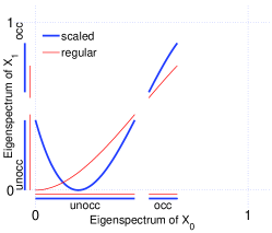
(a)   First iteration

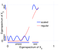
(b)   Third iteration

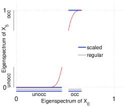
(c)   Fifth iteration

Figure 1: Mapping of the eigenspectrum after 1, 3, and 5 iterations respectively of McWeeny based fixed-$\mu$ purification with and without use of scaling. In this illustrative example $\Delta\epsilon/\xi=10$ and the chemical potential $\mu$ is located at $\lambda_{\textrm{min}}+0.25(\lambda_{\textrm{max}}-\lambda_{\textrm{min}})$.

We will first apply the scale and fold technique to fixed-$\mu$ purification using a polynomial $P_{m,m}$ with $m$ being odd. For such polynomials, the technique can be used to fold both the unoccupied and occupied parts of the eigenspectrum in each iteration. In this case the non-monotonic purification transformation

$$f_{i}(X_{i-1})=P_{m,m}(\alpha(X_{i-1}-0.5)+0.5I)$$ (2)

where $\alpha\geq 1$ determines the amount of scaling around 0.5. The complete algorithm for the special case $m=1$ is given in Algorithm 1, where $\lambda_{\textrm{min}}$ and $\lambda_{\textrm{max}}$ are the extremal eigenvalues of $F$ or bounds thereof. For simplicity, it is assumed here that the band gap is located symmetrically around $\mu$. The expression for $\alpha$ can be derived by solving

$$P_{m,m}(\alpha(\beta-0.5)+0.5)=P_{m,m}(0.5(1-\alpha))$$ (3)

for $\alpha\geq 1$. Here, $\beta$ is a parameter depending on the eigenvalue closest to 0.5, see Algorithm 1. The behavior of Algorithm 1 is illustrated in Figure 1. The behavior of the regular grand-canonical purification algorithm,Palser and Manolopoulos (1998) corresponding to Algorithm 1 with $\alpha=1$, is shown for reference. Note how the scaled variant is able to take advantage of the additional flexibility given by allowing for non-monotonicity, resulting in much faster convergence. Fixed-$\mu$ purification schemes with scaling can also be derived for other polynomials of the form $P_{i,j}$ where $i$ and $j$ are both odd and larger than 0. Note that the scaling should be performed around the unstable fixed point of the polynomial which will differ from 0.5 if $i\neq j$.

Algorithm 1 McWeeny based fixed-$\mu$ purification

1:$F,\lambda_{\textrm{min}},\lambda_{\textrm{max}},\mu,\xi$

2:$\gamma=2\max(\lambda_{\textrm{max}}-\mu,\mu-\lambda_{\textrm{min}})$

3:$X_{0}=\frac{\mu I-F}{\gamma}+0.5I$

4:$\beta=0.5(1-\xi/\gamma)$

5:for  $i=1,2,\dots,n$  do

6:     $\alpha=3/\sqrt{12\beta^{2}-18\beta+9}$

7:     $X_{s}=\alpha(X_{i-1}-0.5I)+0.5I$

8:     $X_{i}=3X_{s}^{2}-2X_{s}^{3}$

9:     $\beta_{s}=\alpha(\beta-0.5)+0.5$

10:     $\beta=3\beta_{s}^{2}-2\beta_{s}^{3}$

11:end for

12:return $D=X_{n}$

Algorithm 2 $P_{0,1}$ & $P_{1,0}$ based varying-$\mu$ purification

1:$F,\lambda_{\textrm{min}},\lambda_{\textrm{max}},\lambda_{\textrm{lumo}},\lambda_{\textrm{homo}}$

2:$X_{0}=f_{0}(F)=(\lambda_{\textrm{max}}I-F)/(\lambda_{\textrm{max}}-\lambda_{\textrm{min}})$

3:$\beta=f_{0}(\lambda_{\textrm{lumo}})$

4:$\bar{\beta}=f_{0}(\lambda_{\textrm{homo}})$

5:for  $i=1,2,\dots,n$  do

6:     if $\beta+\bar{\beta}>1$ then

7:         $\alpha=\beta/(2-\beta)$

8:         $X_{i}=((1+\alpha)X_{i-1}-\alpha I)^{2}$

9:         $\beta=((1+\alpha)\beta-\alpha)^{2}$

10:         $\bar{\beta}=((1+\alpha)\bar{\beta}-\alpha)^{2}$

11:     else

12:         $\alpha=(1-\bar{\beta})/(1+\bar{\beta})$

13:         $X_{i}=2(1+\alpha)X_{i-1}-(1+\alpha)^{2}X_{i-1}^{2}$

14:         $\beta=2(1+\alpha)\beta-(1+\alpha)^{2}\beta^{2}$

15:         $\bar{\beta}=2(1+\alpha)\bar{\beta}-(1+\alpha)^{2}\bar{\beta}^{2}$

16:     end if

17:end for

18:return $D=X_{n}$

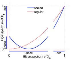
(a)   First iteration

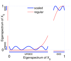
(b)   Fifth iteration

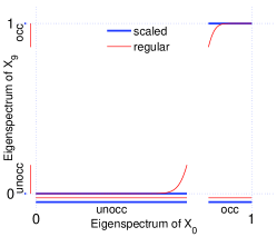
(c)   Ninth iteration

Figure 2: Mapping of the eigenspectrum after 1, 5, and 9 iterations respectively of $P_{0,1}$ & $P_{1,0}$ based varying-$\mu$ purification with and without use of scaling. In this illustrative example $\Delta\epsilon/\xi=10$ and the chemical potential $\mu$ is located at $\lambda_{\textrm{min}}+0.25(\lambda_{\textrm{max}}-\lambda_{\textrm{min}})$.

The scale and fold technique can also be used together with varying-$\mu$ purification. We shall here focus on purification based on the polynomials $P_{0,1}$ and $P_{1,0}$. These polynomials can be used to adjust the occupation count;Niklasson (2002) if the occupation is too high, the $P_{1,0}$ polynomial is applied, otherwise $P_{0,1}$ is applied. The scaling should in this case be chosen to stretch out the eigenspectrum below $0$ before application of $x^{2}$ and above $1$ before application of $2x-x^{2}$. The purification transformations are

$$f_{i}(X_{i-1})=P_{1,0}((1+\alpha)X_{i-1}-\alpha I)$$ (4)

and

$$f_{i}(X_{i-1})=P_{0,1}((1+\alpha)X_{i-1})$$ (5)

where $\alpha\geq 0$ determines the amount of scaling. A complete algorithm is given in Algorithm 2, where $\lambda_{\textrm{lumo}}$ and $\lambda_{\textrm{homo}}$ are the eigenvalues closest above and below the band gap, respectively. Without scaling, i.e. $\alpha=0$, this algorithm is essentially equivalent to the second order trace correcting purification scheme by Niklasson,Niklasson (2002) the only difference being how to choose polynomial in line 5 of the algorithm. In the original work by Niklasson, the choice was based on the trace of the current density matrix approximation. Here, the polynomial is chosen based on the eigenvalues $\beta$ and $\bar{\beta}$ that correspond to the lowest unoccupied and highest occupied molecular orbitals, respectively.Rubensson et al. (2008) The behavior of Algorithm 2 is illustrated in Figure 2. The regular scheme with $\alpha=0$ is shown for reference.

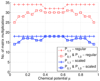
(a)   Varying $\mu$

(b)   Varying $\xi$

Figure 3: Number of matrix-matrix multiplications needed to reach an accuracy of $\|\widetilde{D}-D\|_{2}\leq 10^{-9}$, where $\widetilde{D}$ is the computed approximation of the exact density matrix $D$. The test calculations presented in Panel (a) were performed on test Hamiltonians with band gaps $\xi=0.01$ and varying chemical potential $\mu$. The test calculations presented in Panel (b) were performed on test Hamiltonians with chemical potentials $\mu=0.5$ and varying band gap $\xi$. In all cases, the spectral widths of the test Hamiltonians were $\Delta\epsilon=1$. The test cases in Panel (a) are essentially equivalent to the test cases presented in Figure 2 of Ref. Niklasson, 2002.

Figures 1 and 2 show that the use of scaling results in more rapid convergence. In order to closer study the performance enhancement given by the scaling technique we shall consider diagonal test Hamiltonians with varying chemical potential and band gap. As previously discussed by Maziotti,Mazziotti (2003) the results for a given chemical potential and a given band gap are valid for any Hamiltonian with that band gap and chemical potential.

Figure 3(a) shows that the proposed scaling techniques give significant speedup independently of the location of the chemical potential. As can be seen in Figure 3(b), the cost of the scaled purification schemes scale as $\mathcal{O}(1/\ln\xi)$ with the band gap $\xi$, just as for the regular schemes. However, the convergence for the scaled schemes is around twice as fast as for the regular schemes.

The scaling technique requires some information about the location of the band gap. More precisely, a lower bound of the lower edge and an upper bound of the upper edge of the band gap are needed. It should be noted that incorrect bounds can lead to a mix-up between occupied and unoccupied states. However, even if the bounds are not tight, the scaling technique can be used although the effect will not be as good as it could have been. Tight bounds can be obtained by some technique for calculation of interior eigenvalues.Vömel et al. (2008); Rubensson and Zahedi (2008); Rubensson et al. (2008)

The performance was here measured by the number of matrix-matrix multiplications needed to reach a certain accuracy. In practical linear scaling calculations, efficient ways to bring about sparsity is critical for the performance. Since the proposed schemes are on the standard form given by (1), it is possible to combine them with previously suggested schemes for control of the forward error.Rubensson et al. (2008) As fewer iterations are needed, more aggressive truncation of small matrix elements can be used in each iteration. Therefore, we expect that the speedup given by the proposed techniques will be even better when the additional problem of bringing about sparsity is taken into account, although this is something that needs to be further investigated.

In this letter, non-monotonic recursive polynomial expansions for calculation of the density matrix were proposed. We have withdrawn from the idea that the approximation of the step function should be monotonically increasing and show that this makes it possible to find new, more efficient non-monotonic purification transformations. The scaled purification variants of this work represent a substantial improvement compared to previous purification schemes. The reduction in computational cost is essentially independent of the location of the chemical potential and the proposed schemes are particularly efficient in case of small band gaps.

Comments from Sara Zahedi and support from the Swedish Research Council under Grant No. 623-2009-803 are gratefully acknowledged.

References

- Goedecker (1999) S. Goedecker, Rev. Mod. Phys. 71, 1085 (1999).
- Bowler et al. (2002) D. Bowler, T. Miyazaki, and M. Gillan, J. Phys. 14, 2781 (2002).
- Saad et al. (2010) Y. Saad, J. R. Chelikowsky, and S. M. Shontz, SIAM Review 52, 3 (2010).
- Hine et al. (2009) N. Hine, P. Haynes, A. Mostofi, C.-K. Skylaris, and M. Payne, Comp. Phys. Commun. 180, 1041 (2009).
- Rudberg et al. (2010) E. Rudberg, E. H. Rubensson, and P. Sałek, J. Chem. Theory Comput. (in press) (2010).
- Goedecker and Colombo (1994) S. Goedecker and L. Colombo, Phys. Rev. Lett. 73, 122 (1994).
- Goedecker and Teter (1995) S. Goedecker and M. Teter, Phys. Rev. B 51, 9455 (1995).
- Baer and Head-Gordon (1997) R. Baer and M. Head-Gordon, J. Chem. Phys. 107, 10003 (1997).
- Liang et al. (2003) W. Liang, C. Saravanan, Y. Shao, R. Baer, A. T. Bell, and M. Head-Gordon, J. Chem. Phys. 119, 4117 (2003).
- Palser and Manolopoulos (1998) A. H. R. Palser and D. E. Manolopoulos, Phys. Rev. B 58, 12704 (1998).
- Niklasson (2002) A. M. N. Niklasson, Phys. Rev. B 66, 155115 (2002).
- Niklasson et al. (2003) A. M. N. Niklasson, C. J. Tymczak, and M. Challacombe, J. Chem. Phys. 118, 8611 (2003).
- Holas (2001) A. Holas, Chem. Phys. Lett. 340, 552 (2001).
- Mazziotti (2003) D. A. Mazziotti, Phys. Rev. E 68, 066701 (2003).
- Beylkin et al. (1999) G. Beylkin, N. Coult, and M. J. Mohlenkamp, J. Comput. Phys. 152, 32 (1999).
- Németh and Scuseria (2000) K. Németh and G. E. Scuseria, J. Chem. Phys. 113, 6035 (2000).
- Li et al. (1993) X.-P. Li, R. W. Nunes, and D. Vanderbilt, Phys. Rev. B 47, 10891 (1993).
- Haynes and Payne (1999) P. D. Haynes and M. C. Payne, Phys. Rev. B 59, 12173 (1999).
- Helgaker et al. (2000) T. Helgaker, H. Larsen, J. Olsen, and P. Jørgensen, Chem. Phys. Lett. 327, 397 (2000).
- Shao et al. (2003) Y. Shao, C. Saravanan, M. Head-Gordon, and C. A. White, J. Chem. Phys. 118, 6144 (2003).
- Rudberg and Rubensson (2010) E. Rudberg and E. H. Rubensson, submitted manuscript (2010).
- (22) The McWeeny polynomialMcWeeny (1956) is . This polynomial is equivalent to the Newton-Schulz iteration polynomial for sign matrix evaluation.Higham (2008) The polynomials suggested by HolasHolas (2001) can be written in the form . NiklassonNiklasson (2002) proposed purification schemes based on polynomials and . MaziottiMazziotti (2003) suggested use of asymmetric polynomials and .
- Kenney and Laub (1992) C. Kenney and A. J. Laub, SIAM Journal on Matrix Analysis and Applications 13, 688 (1992).
- Higham (2008) N. J. Higham, Functions of matrices : theory and computation (Society for Industrial and Applied Mathematics, Philadelphia, 2008).
- Rubensson et al. (2008) E. H. Rubensson, E. Rudberg, and P. Sałek, J. Chem. Phys. 128, 074106 (2008).
- Vömel et al. (2008) C. Vömel, S. Z. Tomov, O. A. Marques, A. Canning, L.-W. Wang, and J. J. Dongarra, J. Comput. Phys. 227, 7113 (2008).
- Rubensson and Zahedi (2008) E. H. Rubensson and S. Zahedi, J. Chem. Phys. 128, 176101 (2008).
- McWeeny (1956) R. McWeeny, Proc. R. Soc. London Ser. A 235, 496 (1956).