The spiral spin state in a zigzag spin chain system

Abstract

We considered a spin chain with nearest neighbor and next nearest neighbor exchange interactions, anisotropic exchange interaction and Dzyaloshinskii-Moriya interaction. The conditions of the spiral spin state as the ground state were analyzed. Our purpose is to build the connection between the spiral state and the fully polarized state with a unitary transformation. Under this transformation, anisotropic exchange interaction and Dzyaloshinskii-Moriya interaction can be transformed to each other. Then we use positive semi-definite matrix theorem to identify the region of fully polarized state as the ground state for the transformed Hamiltonian, and it is the region of spiral spin state as the ground state of the original Hamiltonian. We also found that the effect of Dzyaloshinskii-Moriya interaction is important. Its strength is related to the pitch angle of spiral spins. Our method can be applied to coupled spin chains and two dimensional triangular lattice systems. Our results can be compared with the experiment data.

I Introduction

The spiral spin states has been the subject of study for more than sixty years AY59 ; TN62 ; TN59 . Yet it still gives rise to surprising physical properties. We focus on the multiferroic phenomenon found recently in numerous compounds Wan09 . Experiments MK05 ; Che08 showed that in the multiferroic material the magnetic and ferroelectric orders are closely related. What is more intriguing is that only certain types of magnetic orders, can couple to ferroelectricity. Furthermore, only spiral spins configuration gives rise to strong coupling between electric polarization and magnetic order. The spin-current modelHK05 provided a plausible explanation for this phenomenon.

Beside multiferroics, the spiral spin state was found in many other transition metal compounds. In the early studyKim08 ; TS09 , they have presented the evidences of the existence of spiral spin state in multiferroics. In LiCu₂O₂ neutron ; li08 ; li09 and NaCu₂O₂ Na10 , there are one-dimensional spin chains consist of edge-sharing octahedra. The Cu-O-Cu bond angle is almost $90$-degree. This renders the superexchange interaction between nearest neighbor (NN) weak and ferromagnetic Khom96 and the exchange between next nearest neighbor (NNN) not negligible. The spiral spin configuration can also be found in higher dimension systems. The structure of ACrO₂ (A=Cu, Ag, Li, or Na)To08 is a two dimensional triangular lattice, and its bond angle of Cu-O-Cu is also close to $90$-degree. This can also be the cause of the spiral spin state.

The existence of spiral spin configuration can be attributed to the frustration in the system. A relatively simple case is a one-dimensional spin chain with NN and NNN exchange interactions, to be denoted as $J_{1}$ and $J_{2}$ respectively. Frustration is caused by their competing tendencies of aligning spins. This kind of systems is often called zigzag spin chains. There have been much analysis on this subject. Exact solutions have been found for special cases. The most notable case is the dimer state at $J_{1}/J_{2}=2$ found by Majumdar and Ghosh MG69 . At the other end $J_{1}/J_{2}=-4$, it was found that the fully polarized (FP) state and uniformly distributed resonant valence bond state Nat88 are degenerate ground states (GS). In general, the phase diagram is summarized by Bursill RB95 . The boundary of the frustrated region is identified by numerical calculation. White and Affleck White96 calculated the correlation function $\left\langle\overrightarrow{S}_{i}\overrightarrow{S}_{j}\right\rangle$ and provided solid evidence of the existence of the spiral spin state. Furthermore, it has been found that in zigzag spin chains, there exists chiral order TH10 ; IP08 ; KO08 . This is another indication of the extensive existence of spiral spin state. Hence the existence of spiral spin state becomes an important subject.

The spiral spin state can be found in many physical systems. For example, both of neutron diffractionneutron and polarization dependent resonant soft x-ray magnetic scattering (RSXMS)li08 experiments indicate an incommensurate superstructure with $Q=(0.5,0.1738,0)$ at low temperature, where $\vec{Q}$ is the wave vector of spiral spins. In the direction of chain (b-axis) the spiral angle is about $\phi^{\prime}=\vec{Q}\cdot\vec{b}=62^{0}$, which is the angle difference of two adjoint spin. We will show our result in the case of $\phi^{\prime}=50^{0}$ which is comparable to experimental finding. The discrepancy could come from inter-chain coupling. Though we also consider the inter-chain coupling in Sec.V, its magnitude may not be practical. Further work is needed.

Dzyaloshinskii-Moriya (DM) interaction DM58 ; DM60 not only plays an important role in the multiferroic material, but also produces many exotic physical phenomena. It is another mechanism which can give rise to spiral spin state. It can act as a vector potential on the spin wave in the magnon spin Hall effect Hall10 . In ferromagnetic nanowires DM interaction has profound effect on the motion of domain walls AA10 . It can also give rise to spin current and soliton in spin chainsGJA08 . Therefore, it is important to incorporate DM interaction into the model Hamiltonian to see what role it plays.

The purpose of our study is to find the condition for the spiral spin state being the ground state (GS) in zigzag spin chain. In Sec.II, we start with a Hamiltonian with NN, NN and DM interactions and derive the conditions of spiral spin states being the eigen states by performing a unitary transformation. In Sec.III, we use the positive semi-definite (PSD) matrix theorem to determine the conditions of ground state (GS), by decomposing the system into local Hamiltonian. Examples are given in Sec.III.1 and Sec.III.2 to illustrate our result. The problem of symmetry is discussed in Sec.IV. The applications to real physical systems of coupled zigzag spin chain and two-dimensional triangular lattice are given in Sec.V. In Sec. VI, we compare our results with those of numerical calculations and simulations. Sec. VII is devoted to the conclusions.

II Spiral spin state as an eigen state

The physical systems which prefer spiral spin configuration usually have competing interactions. For example, when the nearest neighbor (NN) exchange interaction is weak, the next nearest neighbor (NNN) interaction or even Dzyaloshinskii-Moriya (DM) interaction become relatively significant. The Hamiltonian of this kind of systems (are usually called the zigzag spin chains) can be written as

$$H= \sum_{j}J_{1}[\Delta_{1}s_{j}^{z}s_{j+1}^{z}+\frac{1}{2}(s_{j}^{+}s_{j+1}^{-}+s_{j}^{-}s_{j+1}^{+})$$

$$+D_{1}\vec{s}_{j}\times\vec{s}_{j+1}\cdot\hat{z}]$$

$$+J_{2}[\Delta_{2}s_{i}^{z}s_{j+2}^{z}+\frac{1}{2}(s_{j}^{+}s_{j+2}^{-}+s_{j}^{-}s_{j+2}^{+})$$

$$+D_{2}\vec{s}_{j}\times\vec{s}_{j+2}\cdot\hat{z}]$$ (1)

where $j$ is the label of the lattice site, $J_{1}$ is the NN interaction, $J_{2}$ is the NNN interaction, $\Delta_{1}(\Delta_{2})$ gives the anisotropic interaction along $z$ axis for NN (NNN) interaction, and $D_{1}(D_{2})$ is the DM interaction between NN (NNN).

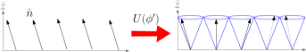
Figure 1: The way to analyze spiral state is to connect it to a fully polarized (FP) state with a unitary transformation, which is the product of rotations around $z$-axis.

Although there have been numerous studies on the zigzag spin chain, the boundary for the spiral spin state being the ground state still cannot be determined if DM interaction is present. Here we propose another way to analyze. We connect the spiral spin state and a fully polarized (FP) state by a unitary transformation. The FP state and the spiral spin state are shown in Fig. 1. We then ask the question: Under what conditions the FP state will be the ground state (GS) of the transformed Hamiltonian? Since under any unitary transformation, the energy spectrum does not change, the ground states of the physical Hamiltonian and transformed Hamiltonian are equivalent. By identifying the region of FP state being GS for the transformed Hamiltonian, we will know the region of spiral spin state as GS of the physical Hamiltonian.

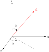
Figure 2: The definition of spin orientation $\hat{n}$, where $\hat{n}=(\sin(\beta)\cos(\alpha),\sin(\beta)\sin(\alpha),\cos(\beta))$.

The unitary transformation mentioned above rotates the spins around the $z$-axisLOA92 . It has the form

$$U(\phi^{\prime})=\prod_{j=1}^{N}\exp(is_{j}^{z}\vec{Q}\cdot\vec{R}_{j}),$$ (2)

with $\phi^{\prime}=\vec{Q}\cdot(\vec{R}_{j+1}-\vec{R}_{j})$ being a constant. For now, $\phi^{\prime}$ and hence, $\vec{Q}$ can have arbitrary values. But, as it will be shown later, the DM interaction has a profound effect on $\phi^{\prime}$ and $\vec{Q}$. For a given strength of DM interaction ($D_{1}$ and $D_{2}$), the boundaries of $\phi^{\prime}$ and $\vec{Q}$ are determined. Within the boundaries, the spiral spin states are the ground states of the system. Hence, the spiral spin state

$$|\psi_{ss}\rangle=\prod_{j=1}^{N}[\cos(\frac{\beta}{2})|\uparrow\rangle_{j}+\sin(\frac{\beta}{2})e^{i(\vec{Q}\cdot\vec{R}_{j}-\alpha)}|\downarrow\rangle_{j}],$$

can be transformed into a FP state with spin direction $\hat{n}=(\sin(\beta)\cos(\alpha),\sin(\beta)\sin(\alpha),\cos(\beta))$ (see Fig. 2), as the following form

$$|FP,\hat{n}\rangle=\prod_{j=1}^{N}[\cos(\frac{\beta}{2})|\uparrow\rangle_{j}+\sin(\frac{\beta}{2})e^{-i\alpha}|\downarrow\rangle_{j}].$$ (3)

The Hamiltonian is also transformed

$$H_{rot}=UHU^{-1}$$

$$=\sum_{j} [J_{1}(\Delta_{1}s_{j}^{z}s_{j+1}^{z}+\frac{\cos(\phi_{1}-\phi^{\prime})}{2\cos(\phi_{1})}(s_{j}^{+}s_{j+1}^{-}+s_{j}^{-}s_{j+1}^{+})$$

$$+\frac{\sin(\phi_{1}-\phi^{\prime})}{\cos(\phi_{1})}\vec{s}_{j}\times\vec{s}_{j+1}\cdot\hat{z})$$

$$+J_{2}(\Delta_{2}s_{j}^{z}s_{j+1}^{z}+\frac{\cos(\phi_{2}-2\phi^{\prime})}{2\cos(\phi_{2})}(s_{j}^{+}s_{j+2}^{-}+s_{j}^{-}s_{j+2}^{+})$$

$$+\frac{\sin(\phi_{2}-2\phi^{\prime})}{\cos(\phi_{2})}\vec{s}_{j}\times\vec{s}_{j+2}\cdot\hat{z})]$$

where we have set $\phi_{1}=\tan^{-1}(D_{1}),\phi_{2}=\tan^{-1}(D_{2})$, and used the identity $1+i\tan(\phi)=\sec(\phi)e^{i\phi}$.

In order that $|FP,\hat{n}\rangle$ is an eigen-state of the transformed Hamiltonian, it is required that

$$\Delta_{1} =\frac{\cos(\phi_{1}-\phi^{\prime})}{\cos(\phi_{1})},$$ (4)

$$\Delta_{2} =\frac{\cos(\phi_{2}-2\phi^{\prime})}{\cos(\phi_{2})}.$$ (5)

The constraints give the limitation of the method, i.e., only under these conditions we can proceed further. On the other hand, the constraints show the relation between the spiral angle and the anisotropic exchange interaction. As a result of Eq. (4) and Eq. (5), $H_{rot}$ becomes an isotropic Hamiltonian

$$H_{iso}= \sum_{j}J_{1}\Delta_{1}[\vec{s}_{j}\cdot\vec{s}_{j+1}+D_{1}^{\prime}\vec{s}_{j}\times\vec{s}_{j+1}\cdot\hat{z}]$$

$$+J_{2}\Delta_{2}[\vec{s}_{j}\cdot\vec{s}_{j+2}+D_{2}^{\prime}\vec{s}_{j}\times\vec{s}_{j+2}\cdot\hat{z}]$$ (6)

where $D_{1}^{\prime}=\tan(\phi_{1}-\phi^{\prime}),D_{2}^{\prime}=\tan(\phi_{2}-2\phi^{\prime})$.

As the anisotropy exchange interaction is “rotated ”away for both NN and NNN interaction, it is readily shown that $|FP,\hat{n}\rangle$ is an eigen state of $H_{iso}$ with the relation

$$\sum_{i}\vec{s}_{i}\times\vec{s}_{j}\cdot\hat{z}|FP;\hat{n}\rangle=0.$$

To prove the above equation, one only has to rotate $\hat{n}$ to $\hat{z}$ and $\hat{z}$ to another direction. A more detailed analysis will be given in Sec. IV where the symmetry of the system is also discussed. As a result,

$$H_{iso}|FP,\hat{n}\rangle=E_{0}|FP,\hat{n}\rangle$$ (7)

where $E_{0}=N(J_{1}\Delta_{1}+J_{2}\Delta_{2})/4$. In fact, Eqs. (4) and (5) combined is the requirement that NN and NNN exchange interaction with anisotropy can be transformed into isotropic exchange interactions simultaneously.

III Spiral state as the ground state

In this section, we will identify the region of FP state as the GS in $H_{iso}$ (correspond to the spiral state as GS in $H$ ) by decomposing the Hamiltonians into local Hamiltonians and applying positive semi-definite theorem for analyzing. This methodCSH had been applied to zigzag spin chains without DM interaction. It can also be applied to spin of any length. Here we focus on spin-$1/2$ system.

We dissect the Hamiltonian into many local Hamiltonians as shown in Fig. 3. Each local Hamiltonian contains three spins. Thus, the original Hamiltonian can be written as

$$H_{iso} =\sum_{j=1}^{N}h_{j,j+1,j+2}$$

$$=h_{1,2,3}\otimes\hat{1}_{2^{N-3}}+\sum_{j=2}^{N-2}\hat{1}_{2^{j-1}}\otimes h_{j,j+1,j+2}\otimes\hat{1}_{2^{N-2-j}}$$

$$+\hat{1}_{2^{N-3}}\otimes h_{N-1,N,1}+\hat{1}_{2^{N-3}}\otimes h_{N,1,2}$$ (8)

where the local Hamiltonian is giving by

$$h_{j,j+1,j+2} =\frac{J_{1}\Delta_{1}}{2}[(\vec{s}_{j}+\vec{s}_{j+2})\cdot\vec{s}_{j+1}]+J_{2}\Delta_{2}\vec{s}_{j}\cdot\vec{s}_{j+2}$$

$$+\frac{J_{1}\Delta_{1}D_{1}^{\prime}}{2}[\vec{s}_{j}\times\vec{s}_{j+1}+\vec{s}_{j+1}\times\vec{s}_{j+2}]\cdot\hat{z}$$

$$+J_{2}\Delta_{2}D_{2}^{\prime}\vec{s}_{j}\times\vec{s}_{j+2}\cdot\hat{z}$$ (9)

and $\hat{1}_{M}$ denotes the identity matrix of rank $M$. The direct product of $h_{j,j+1,j+2}$ and $\hat{1}_{M}$ is meant to enlarge the vector space to $2^{N}$ dimension to accommodate $N$ spins. The direct sum gives a Hamiltonian matrix of $2^{N}$ dimension, as shown in Fig. 3. If FP state of three spins is an eigen state of $h_{j,j+1,j+2}$, then that of $N$ spins is an eigen state of $H_{iso}$. Furthermore, if a state of three spins has the lowest energy under $H_{j,j+1,j+2}$, then corresponding state (constructed by direct product) is the GS of $H_{iso}$. This is implied by the theorem of positive semi-definite matrix discussed below.

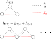
Figure 3: The Hamiltonian can be decomposed into local Hamiltonians, and each local Hamiltonian contains only the interactions between three neighboring spins.

To find the region for a FP state with spin direction $\widehat{n}$ as the ground state of Eq. (8), we rotate the $z$-axis to direction $\hat{n}^{\prime}=(\sin(\beta)\cos(-\alpha),\sin(\beta)\sin(-\alpha),\cos(\beta))$ and $\hat{n}$ to $\hat{z}$. The Hamiltonian of $H_{iso}$ in Eq. (9) becomes

$$h_{j,j+1,j+2}^{\hat{n}^{\prime}} =\frac{J_{1}\Delta_{1}}{2}[(\vec{s}_{j}+\vec{s}_{j+2})\cdot\vec{s}_{j+1}]+J_{2}\Delta_{2}\vec{s}_{j}\cdot\vec{s}_{j+2}$$

$$+\frac{J_{1}\Delta_{1}D_{1}^{\prime}}{2}[\vec{s}_{j}\times\vec{s}_{j+1}+\vec{s}_{j+1}\times\vec{s}_{j+2}]\cdot\hat{n^{\prime}}$$

$$+J_{2}\Delta_{2}D_{2}^{\prime}\vec{s}_{j}\times\vec{s}_{j+2}\cdot\hat{n^{\prime}}.$$

and

$$h_{j,j+1,j+2}^{\hat{n}^{\prime}}|\uparrow\rangle_{j}|\uparrow\rangle_{j+1}|\uparrow\rangle_{j+2}$$

$$=s^{2}(J_{1}\Delta_{1}+J_{2}\Delta_{2})|\uparrow\rangle_{j}|\uparrow\rangle_{j+1}|\uparrow\rangle_{j+2}$$

$$+\frac{\sqrt{2s}s}{4i}\sin(\beta)e^{-i\alpha}(\frac{J_{1}\Delta_{1}D_{1}^{\prime}}{2}+J_{2}\Delta_{2}D_{2}^{\prime})$$

$$\times\left(|\uparrow\rangle_{j}|\uparrow\rangle_{j+1}|\downarrow\rangle_{j+2}-|\downarrow\rangle_{j}|\uparrow\rangle_{j+1}|\uparrow\rangle_{j+2}\right)$$

where $D_{1}^{\prime}=\tan(\phi_{1}-\phi^{\prime}),D_{2}^{\prime}=\tan(\phi_{2}-2\phi^{\prime})$. It is found that for $|\uparrow\rangle_{j}|\uparrow\rangle_{j+1}|\uparrow\rangle_{j+2}$ to be an eigen state, the required relation is

$$\frac{J_{1}\Delta_{1}}{J_{2}\Delta_{2}}=\frac{-2D_{2}^{\prime}}{D_{1}^{\prime}}.$$ (10)

This procedure is not restricted to spin one-half systems. Substituting Eq. (10) into Eq. (9), the local Hamiltonian becomes

$$h_{j,j+1.j+2}=J_{2}\Delta_{2} [-\frac{D_{2}^{\prime}}{D_{1}^{\prime}}(\vec{s}_{j}+\vec{s}_{j+2})\cdot\vec{s}_{j+1}+\vec{s}_{j}\cdot\vec{s}_{j+2}$$

$$-D_{2}^{\prime}(\vec{s}_{j}\times\vec{s}_{j+1}+\vec{s}_{j+1}\times\vec{s}_{j+2})\cdot\hat{z}$$

$$+D_{2}^{\prime}\vec{s}_{j}\times\vec{s}_{j+2}\cdot\hat{z}]$$ (11)

To find the region for FP state to be the ground state of this local Hamiltonian, we applied the positive semi-definite theorem. The theorem of positive semi-definite (PSD) matrix is described by the following: The necessary and sufficient condition for a real symmetric matrix $A$ to be positive semi-definite is $x^{T}Ax\geq 0$ for all real vectors $x$. If $M$ and $N$ are positive semi-definite, then the sum $M+N$, the direct sum $M\oplus N,$ and direct product $M\otimes N$ are also positive semi-definite. Hence, if we are able to prove that $(h_{i,i+1,i+2}-E_{0})$ is a PSD matrix with $E_{0}$ being the energy of the FP state, then the $H_{iso}-E_{0}$ is also a PSD matrix. For spin 1/2 system, the Hamiltonian in Eq. (11) is $2^{3}\times 2^{3}$ matrix. Its energy spectrum is

$$E_{0} \mbox{ with four fold degeneracy};$$

$$E_{0}+\delta E_{1}$$ with two fold degeneracy

$$E_{0}+\delta E_{2}$$ with two fold degeneracy (12)

where $E_{0}$ is the energy of FP state, and

$$\frac{\delta E_{1}}{J_{2}\Delta_{2}} =\frac{2D_{1}^{\prime}D_{2}^{\prime}-D_{1}^{\prime 2}-\sqrt{\left[3D_{1}^{\prime 2}D_{2}^{\prime 2}+(D_{1}^{\prime}+D_{2}^{\prime 2})\right]D_{1}^{\prime 2}}}{2D_{1}^{\prime 2}}$$

$$\frac{\delta E_{2}}{J_{2}\Delta_{2}} =\frac{2D_{1}^{\prime}D_{2}^{\prime}-D_{1}^{\prime 2}+\sqrt{\left[3D_{1}^{\prime 2}D_{2}^{\prime 2}+(D_{1}^{\prime}+D_{2}^{\prime 2})\right]D_{1}^{\prime 2}}}{2D_{1}^{\prime 2}}$$

To make local Hamiltonian a PSD matrix, one requires $\delta E_{1}\geq 0$ and $\delta E_{2}\geq 0$. Therefore the conditions for PSD are

$$\Big{\{}\begin{array}[c]{ll}\quad(1-D_{1}^{\prime 2})D_{2}^{\prime 2}\geq 2D_{1}^{\prime}D_{2}^{\prime}\mbox{ and }2D_{1}^{\prime}D_{2}^{\prime}\geq D_{1}^{\prime 2}&\mbox{for }J_{2}\Delta_{2}\geq 0\\ \mbox{or}&\\ \quad(1-D_{1}^{\prime 2})D_{2}^{\prime 2}\leq 2D_{1}^{\prime}D_{2}^{\prime}\mbox{ and }2D_{1}^{\prime}D_{2}^{\prime}\leq D_{1}^{\prime 2}&\mbox{for }J_{2}\Delta_{2}\leq 0.\end{array}$$ (13)

This is the end of our derivation. Summarizing briefly, Eq. (4) and Eq. (5) are the conditions of FP states being the eigen states of $H_{ios}$ in Eq. (3). Hence they are also the conditions of the spiral spin states being the eigen states of the physical Hamiltonian in Eq. (1). On the other hand, Eq. (10) and inequality (13) are the conditions of the spiral spin states being the ground states of the physical Hamiltonian in Eq. (1).

For most insulating compounds, $J_{2}$, the NNN superexchange interaction is antiferromagnetic. Hence, we consider the case $J_{2}>0$ and $\Delta_{2}\geq 0$. The region for PSD in Eq. (13) can also be written as

$$\Big{\{}\begin{array}[c]{ll}2\phi^{\prime}-\frac{\pi}{2}\leq\phi_{2}\leq 2\phi^{\prime}&\mbox{ for }\frac{\phi_{2}}{2}\leq\phi_{1}\leq\phi^{\prime}\\ 2\phi^{\prime}\leq\phi_{2}\leq 2\phi^{\prime}+\frac{\pi}{2}&\mbox{ for }\phi^{\prime}\leq\phi_{1}\leq\frac{\phi_{2}}{2}+\frac{\pi}{2}\end{array}$$

It is indicated by the shaded area in Fig. 4, for a given $\phi^{\prime}$. Fig. 4 shows the main result of this work. In view of Eq. (4), Eq. (5) and Eq. (10), we see that there are two free parameters in Eq. (1), namely $\phi_{1}(D_{1})$ and $\phi_{2}(D_{2})$. In the parameter space of $\phi_{1}$ and $\phi_{2}$, the shaded regions show where spiral spin states are the ground states. The pitch angle $\phi^{\prime}$ of the spiral spins is closely related to the values of $\phi_{1}(D_{1})$ and $\phi_{2}(D_{2})$. Hence, the DM interaction plays the crucial role of determining the existence of spiral spin states.

It has been shown that inside the shaded region of Fig. 5, the spiral spin states are the ground state. However, we also found that there are gapless excitations or Goldstone modes (details are in sec. IV). Outside the boundary, these modes actually have lower energy as it will show in Eq. (19). Hence, the spiral spin states are the ground states in the shaded region. But they are not the ground states outside of these boundaries which are exact since our solution is exact. On the other hand, it is possible that the chiral correlation or the in-plane spin correlation still exhibit long-range order behavior outside of the boundaries. Furthermore, we cannot rule out the possibility of the spiral spin states being the ground states in some other region in phase space which is not in the neighborhood of the shaded regions.

For later use, we will show some cases explicitly in Fig. 5, the shaded regions will correspond to the condition for spiral GS. In the following, we give two simple examples to illustrate our result.

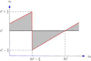
Figure 4: The shaded regions show where spiral spin states are the ground states and the relation between the pitch angle and $(\phi_{1},\phi_{2})$ in the Hamiltonian, and the region for shifting $\pi$ in both $(\phi_{1}$ and $\phi_{2})$ axes are also the PSD region.

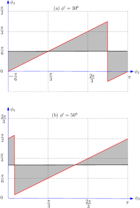
Figure 5: The shaded regions show where spiral spin states are the ground states and the relation between the pitch angle and $(\phi_{1},\phi_{2})$ in the Hamiltonian, for (a)$\phi^{\prime}=30^{0}$, (b)$\phi^{\prime}=50^{0}$.

Similarly, for spin-s system of the Hamiltonian, the local site Hamiltonian is a $(2s+1)^{3}\times(2s+1)^{3}$ matrix. After diagonalization, the energy spectrum can be obtained. The theorem of PSD matrix can also give the region for FP state as GS. Hence the result of this section can be generalized to spins of any possible length.

III.1 Isotropic exchange interaction

For physical systems having isotropic superexchange, or $\Delta_{1}=\Delta_{2}=1$ (in our case $\phi_{1}=\frac{\phi^{\prime}}{2},\phi_{2}=\phi^{\prime}$), the Hamiltonian of Eq.(1) becomes

$$H^{\prime}=J_{2} \sum_{i}-2\frac{\tan(\phi^{\prime})}{\tan(\frac{\phi^{\prime}}{2})}\vec{s}_{i}\cdot\vec{s}_{i+1}+\vec{s}_{i}\cdot\vec{s}_{i+2}$$

$$-\tan(\phi^{\prime})(2\vec{s}_{i}\times\vec{s}_{i+1}-\vec{s}_{i}\times\vec{s}_{i+2})\cdot\hat{z}$$

The conditions for PSD of Eq.(13) turn out to be

$$\phi^{\prime}=\Big{\{}\begin{array}[c]{cc}0^{0}\sim 90^{0},270^{0}\sim 360^{0}&\mbox{ with }J_{2}>0,\\ 90^{0}\sim 270^{0}&\mbox{ with }J_{2}<0.\end{array}$$ (14)

So in physical case $J_{2}>0$, the spiral angle $\phi^{\prime}$ is in the range $0^{0}\sim 90^{0}$ or $270^{0}\sim 360^{0}$.

The implication of Eq. (14) can be seen by considering the following three simple cases: (a) $\phi^{\prime}=0^{0}$, or the GS is the FP state. In this case $H^{\prime}=J_{2}\sum_{i}-4\vec{s}_{i}\cdot\vec{s}_{i+1}+\vec{s}_{i}\cdot\vec{s}_{i+2}$. It has been shown Nat88 that the FP state and the UDRVB state are degenerate GS. Our method correctly leads to one of them. (b) $\phi^{\prime}=\pi$, or the GS is the Neel state. In this case $H^{\prime}=-|J_{2}|\sum_{i}\vec{s}_{i}\cdot\vec{s}_{i+2}$. The system becomes two decoupled spin chains. Each is ferromagnetically coupled. (c) The GS is spiral state with spiral angle being $30^{0}$. The resulting parameters are $(J_{1},J_{2},\Delta_{1},\Delta_{2},D_{1},D_{2})=(-4.13,1,1,10.268,0.577)$. (d) For specific spiral angle $\phi^{\prime}=50^{0}$, the resulting parameters are $(J_{1},J_{2},\Delta_{1},\Delta_{2},D_{1},D_{2})=(-5.111,1,1,1,0.466,1.191)$.

In this isotropic Hamiltonian, the relative strength of exchange coupling is $J_{1}/J_{2}=-2\tan(\phi^{\prime})/\tan(\phi^{\prime}/2)$. In the region of PSD in Eq. (14) with $J_{2}>0$, this is always less than $-4$. We shall see in Sec. V that for coupled spin chains or two-dimensional cases, the superexchange $J_{1}/J_{2}$ can be tuned by inter chain coupling $J_{3}$ to make $|J_{1}/J_{2}|$ smaller.

III.2 Without DM interaction

For system containing high symmetry or small spin-orbital interaction, we have the case $D_{1}\approx D_{2}\approx 0$, implying $\phi_{1}=\phi_{2}=0$. Then the Hamiltonian in Eq. (1) under the condition of Eqs. (4,5,10) becomes

$$H^{\prime\prime}=J_{2} \sum_{j}-4\cos(\phi^{\prime})(\cos(\phi^{\prime})s_{j}^{z}s_{j+1}^{z}+s_{j}^{x}s_{j+1}^{x}+s_{j}^{y}s_{j+1}^{y})$$

$$+(\cos(2\phi^{\prime})s_{j}^{z}s_{j+2}^{z}+s_{j}^{x}s_{j+2}^{x}+s_{j}^{y}s_{j+2}^{y})$$ (15)

and the spiral state is the eigen state. Now we have

$$\frac{J_{1}}{J_{2}}=-4\cos(\phi^{\prime}),$$ (16)

which is consist with the result of treating spins as classic vectors.

Here are several examples of the system in Eq. (15): (a) For GS with pitch angle $\phi^{\prime}=30^{0}$, the Hamiltonian has parameters $(J_{1},J_{2},\Delta_{1},\Delta_{2},D_{1},D_{2})=(-3.464,1,0.866,0.5,0,0)$. (b) For GS with specific pitch angle $\phi^{\prime}=50^{0}$, the Hamiltonian has parameter $(J_{1},J_{2},\Delta_{1},\Delta_{2},D_{1},D_{2})=(-2.571,1,0.643,-0.174,0,0)$.

The spiral spin state is always the ground state provided the anisotropy interactions between NN and NNN have the forms in Eq. (15) with $J_{2}>0$. However, this kind of solution may not be possible for multiferroics LiCu₂O₂ with $\phi^{\prime}=62^{0}$, because in this case $\Delta_{2}=\cos(124^{0})<0$, and it is likely to be unpractical. It will be shown later, even if inter-chain coupling is considered, $\Delta_{2}$ remains negative. This suggest that there is DM interaction in LiCu₂O₂.

III.3 Special case with $\phi^{\prime}=50^{0}$

For multiferroic compound LiCu₂O₂, the spiral angle is close to $\pi/3$, therefore here we consider this special case. DM interaction and anisotropy are likely to be small. The parameter set $\{(J_{1},J_{2}),(\Delta_{1},\Delta_{2}),(D_{1},D_{2})\}=\{(-3.111,1),(1,0),(0.176,0.176)\}$ gives us $\phi^{\prime}=50^{0}$, which is close to $\pi/3$. However, we note that $\Delta_{2}$ vanishes in this case. We suggest that one can treat $J_{2}\Delta_{2}s_{i}^{z}s_{i+1}^{z}$ as a perturbation. Since $J_{2}\Delta_{2}>0$, the perturbed state should have greater spiral angle. Hence, our approach should to be capable of dealing with realistic physical system such as LiCu₂O₂. The same approach can be used for other value of spiral angle $\phi^{\prime}$.

IV Symmetry properties

In Sec. II, we showed that FP state in Eq. (7) for any direction $\hat{n}$ is an eigen state. Later in Sec. III, we identified the region for these states to be GS. These states form a Hilbert space which has SU(2) symmetry. We can implement a site-dependent unitary rotation (O(2) rotation) to generate spiral states. On the other hand, the Hamiltonians $H$, $H_{rot}$ and $H_{iso}$ all have only $SO(2)$ symmetry. Hence, we arrived at a situation which is called ”emergent symmetry” by Batista Ba09 . The symmetry group of the Hamiltonian in Eq. (1) is isomorphic to that of $H_{iso}$ which is $SO(2)$. However, the Hilbert space of degenerate spiral states has a symmetry group which is isomorphic to $SU(2)$. We give a detailed analysis in this section.

To see the symmetry property of this system more clearly, we first express our results following the notations of Batista Ba09 . We note in passing that our result contain DM interaction, which is a generalization. The Hamiltonian of Eq.(1) in $k$-space is

$$H=\sum_{q} [J_{1}\Delta_{1}\cos(q)+J_{2}\Delta_{2}\cos(2q)]s_{q}^{z}s_{-q}^{z}$$

$$+[J_{1}(\cos(q)-D_{1}\sin(q))$$

$$+J_{2}(\cos(2q)-D_{2}\sin(2q))]s_{q}^{+}s_{q}^{-}$$ (17)

where $s_{q}^{z}=\frac{1}{\sqrt{L}}\sum_{j}e^{iqj}s_{j}^{z},s_{q}^{+}=\frac{1}{\sqrt{L}}\sum_{j}e^{iqj}s_{j}^{+}$, and $s_{q}^{-}=(s_{q}^{+})^{\dagger}$, with lattice constant set to $1$. The commutation relation of $s_{q=\phi^{\prime}}^{\dagger}$ is

$$[s_{\phi^{\prime}}^{+},H]=\frac{i}{\sqrt{L}}\sum_{l}e^{il\phi^{\prime}}s_{l}^{+}a_{l}$$

where

$$a_{l} =\frac{J_{1}\sin(\phi_{1}-\phi^{\prime})}{\cos(\phi_{1})}(s_{l+1}^{z}-s_{l-1}^{z})$$

$$+\frac{J_{2}\sin(\phi_{2}-2\phi^{\prime})}{\cos(\phi_{2})}(s_{l+2}^{z}-s_{l-2}^{z})$$

From $H|FP,-\hat{z}\rangle=E_{0}|FP,-\hat{z}\rangle$ and $a_{l}|FP,-\hat{z}\rangle=0$, we get the relation of $H$ in Eq.(17) as

$$[s_{\phi^{\prime}}^{+},(H-E_{0})](s_{\phi^{\prime}}^{+})^{p}|FP,-\hat{z}\rangle=0$$

for any integer $p$. Hence, $(s_{\phi^{\prime}}^{+})^{p}|FP,-\hat{z}\rangle$ is one of the degenerate eigen states of $H$. The spiral spin states is a linear combination of $(s_{\phi^{\prime}}^{+})^{p}|FP,\hat{z}\rangle$, we show it more directly below.

It is clearer to discuss the symmetry property by analyze the transformed Hamiltonian. The FP states are the degenerate GS of $H_{iso}$ irrespective of the direction of $\hat{n}$. To put it in another way, $H_{iso}$ commute with $\sum_{i}s_{i}^{z}$ so that the $z$-component of the total spin is a good quantum number, hence, they have the following eigen states

$$\{|0\rangle,\sum_{j}|j\rangle,\sum_{j<k}|j,k\rangle,\sum_{j<k<l}|j,k,l\rangle,\dots,|FP;\hat{z}\rangle\}$$ (18)

where $|j,k,\dots\rangle\equiv S_{j}^{+}S_{k}^{+}\dots|0\rangle$ and $|0\rangle\equiv|FP;-\hat{z}\rangle$. Since any FP state $|FP,\hat{n}\rangle$ is a linear combination of the above states, the states in Eq. (18) are actually degenerate GS of $H_{iso}$. Under the unitary transformation, the above states can be transformed into magnon states:

$$\{|0\rangle,s_{\phi^{\prime}}^{+}|0\rangle,(s_{\phi^{\prime}}^{+})^{2}|0\rangle,(s_{\phi^{\prime}}^{+})^{3}|0\rangle,\dots,|FP;\hat{z}\rangle\}$$

The states $(s_{\phi^{\prime}}^{+})^{p}|FP,-\hat{z}\rangle$, those in Eq.(18) and $|FP;\hat{n}\rangle$ are three basis of the degenerate GS of the Hamiltonian in Eq. (1). Each set form a Hilbert space with a symmetry group isomorphic to SU(2) which contains the symmetry group (isomorphic to SO(2)) of the Hamiltonian.

As for the excitation energy of the Hamiltonian in Eq. (1), consider one magnon with wave vector $k$ as $|\psi\rangle=\sum_{j}e^{ikj}|j\rangle$. Using the relation

$$(H-NE_{0})|j\rangle=-(J_{1}\Delta_{1}+J_{2}\Delta_{2})|j\rangle$$

$$+\frac{J_{1}}{2}[(1+iD_{1})|j-1\rangle+(1-iD_{1})|j+1\rangle]$$

$$+\frac{J_{2}}{2}[(1+iD_{2})|j-2\rangle+(1-iD_{2})|j+2\rangle]$$

we found that $|\psi\rangle$ is an eigen state and its energy spectrum is

$$w_{k} =E-NE_{0}$$

$$=J_{1}(\cos(k)-\Delta_{1}+D_{1}\sin(k))$$

$$+J_{2}(\cos(2k)-\Delta_{2}+D_{2}\sin(2k)).$$ (19)

When $k$ approaches $\phi^{\prime}$, the energy $E$ converges to $E_{0}$. Hence we have gapless excitation. Note that the one-magnon states are not the only low-lying excitations. In fact, there are certain two-magnon, multiple-magnon states that are also gapless excitation. Studying on this topic will be presented in another paper.

V Extension of the model

Our result can be generalized to the cases of coupled spin chains and certain types of two-dimensional triangular lattices. Hence, physical systems such as LiCu₂O₂ and ACrO₂(A=Cu,Ag,Li or Na) can be studied with our method.

V.1 Coupled spin-1/2 zigzag spin system

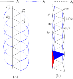
Figure 6: (a) Two coupled zigzag spin chains. (b) Two basic elements denoted as a blue (light) triangular and a red (dark) triangular for two coupled spin chains.

Recently, the compound LiCu₂O₂ li08 ; li09 attracted researchers’ attention because of its multiferroic property. It has chains of edge-sharing oxygen plaquettes with copper ions at the centers. The NN and NNN superexchange interactions strength between copper ions are comparable. A coupled zigzag spin ladder with two legs are shown in Fig. 6(a). The model Hamiltonian is given by

$$H^{csc}= \sum_{j}J_{1}[\Delta_{1}s_{j}^{z}s_{j+2}^{z}+\frac{1}{2}(s_{j}^{+}s_{j+2}^{-}+s_{j}^{-}s_{j+2}^{+})$$

$$+D_{1}\vec{s}_{j}\times\vec{s}_{j+2}\cdot\hat{z}]$$

$$+J_{2}[\Delta_{2}s_{j}^{z}s_{j+4}^{z}+\frac{1}{2}(s_{j}^{+}s_{j+4}^{-}+s_{j}^{-}s_{j+4}^{+})$$

$$+D_{2}\vec{s}_{j}\times\vec{s}_{j+4}\cdot\hat{z}]$$

$$+J_{3}[\Delta_{3}s_{j}^{z}s_{j+1}^{z}+\frac{1}{2}(s_{j}^{+}s_{j+1}^{-}+s_{j}^{-}s_{j+1}^{+})$$

$$+D_{3}\vec{s}_{j}\times\vec{s}_{j+1}\cdot\hat{z}]$$ (20)

where $j$ is the label of the lattice site, $J_{1}$ is the nearest neighbor (NN) interaction, $J_{2}$ the next nearest neighbor (NNN) interaction, $J_{3}$ is the inter-chain coupling, $\Delta_{1}(\Delta_{2},\Delta_{3})$ is the anisotropic interaction along $z$ axis for NN (NNN, inter-chain) interaction and $D_{i}^{\prime}s$ are the respective strength of DM interaction. Superscript $csc$ denotes coupled spin chain. With similar procedure in Sec.II, we set $D_{1}=\tan(\phi_{1}),D_{2}=\tan(\phi_{2}),D_{3}=\tan(\phi_{3})$, and construct the unitary transformation rotating the spins around $z$-axis: $U=\prod_{j=1}^{N}\exp(is_{j}^{z}\vec{Q}\cdot\vec{R}_{j})$ with a constant $\phi^{\prime}=2\vec{Q}\cdot(\vec{R}_{j+1}-\vec{R}_{j})$. The spiral angle is shown in Fig. 6(b). This gives a fixed phase difference between two chains. The conditions of finding a unitary transformation $U(\phi^{\prime})$ to change $H$ into an isotropic Hamiltonian are

$$\Delta_{1} =\frac{\cos(\phi_{1}-\phi^{\prime})}{\cos(\phi_{1})},$$

$$\Delta_{2} =\frac{\cos(\phi_{2}-2\phi^{\prime})}{\cos(\phi_{2})},$$

$$\Delta_{3} =\frac{\cos(\phi_{3}-\frac{\phi^{\prime}}{2})}{\cos(\phi_{3})}.$$

The resulting isotropic Hamiltonian is

$$H_{iso}^{csc}= \sum_{j}J_{1}\Delta_{1}[\vec{s}_{j}\cdot\vec{s}_{j+2}+D_{1}^{\prime}\vec{s}_{j}\times\vec{s}_{j+2}\cdot\hat{z}]$$

$$+J_{2}\Delta_{2}[\vec{s}_{j}\cdot\vec{s}_{j+4}+D_{2}^{\prime}\vec{s}_{j}\times\vec{s}_{j+4}\cdot\hat{z}]$$

$$+J_{3}\Delta_{3}[\vec{s}_{j}\cdot\vec{s}_{j+1}+D_{3}^{\prime}\vec{s}_{j}\times\vec{s}_{j+1}\cdot\hat{z}]$$

where $D_{1}^{\prime}=\tan(\phi_{1}-\phi^{\prime}),D_{2}^{\prime}=\tan(\phi_{2}-2\phi^{\prime})$, and $D_{3}^{\prime}=\tan(\phi_{3}-\frac{\phi^{\prime}}{2})$. If for Hamiltonian $H_{iso}^{csc}$, FP states are the eigen states then for Hamiltonian $H^{csc}$, spiral states are the eigen states.

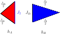
Figure 7: The two basic elements of the system:red (dark) triangles $h_{A}$ and blue (light) triangles $h_{B}$.

We again dissect $H_{iso}^{csc}$ into local Hamiltonians, each contains three spins. However, now there are two kinds of local Hamiltonians, represented by blue (light) and red (dark) triangles in Fig. 6(b). Since the two triangles have a common edge, we divide $J_{1}$ into $J_{1a}$ and $J_{1b}$. This division is arbitrary. As shown in Fig. 7, the two local Hamiltonians are $h_{A}$ (dark or red)and $h_{B}$ (light or blue:)

$$h_{A} =\frac{J_{1a}\Delta_{1}}{2}[(\vec{s}_{i}+\vec{s}_{i+4})\cdot\vec{s}_{i+2}]+J_{2}\Delta_{2}\vec{s}_{i}\cdot\vec{s}_{i+4}$$

$$+\frac{J_{1a}\Delta_{1}D_{1}^{\prime}}{2}[\vec{s}_{i}\times\vec{s}_{i+2}+\vec{s}_{i+2}\times\vec{s}_{i+4}]\cdot\hat{z}$$

$$+J_{2}\Delta_{2}D_{2}^{\prime}\vec{s}_{i}\times\vec{s}_{i+4}\cdot\hat{z},$$ (21)

$$h_{B} =\frac{J_{3}\Delta_{3}}{2}[(\vec{s}_{i}+\vec{s}_{i+2})\cdot\vec{s}_{i+1}]+J_{1b}\Delta_{1}\vec{s}_{i}\cdot\vec{s}_{i+2}$$

$$+\frac{J_{3}\Delta_{3}D_{3}^{\prime}}{2}[\vec{s}_{i}\times\vec{s}_{i+1}+\vec{s}_{i+1}\times\vec{s}_{i+2}]\cdot\hat{z}$$

$$+J_{1b}\Delta_{1}D_{1}^{\prime}\vec{s}_{i}\times\vec{s}_{i+2}\cdot\hat{z}.$$ (22)

$|FP,\hat{n}\rangle$ will be the eigen state locally, provided the following conditions which are analogous to that in Eq. (10), are satisfied by

$$\frac{J_{1a}}{J_{2}} =\frac{-2D_{2}^{\prime}\Delta_{2}}{D_{1}^{\prime}\Delta_{1}},$$ (23)

$$\frac{J_{3}}{J_{1b}} =\frac{-2D_{1}^{\prime}\Delta_{1}}{D_{3}^{\prime}\Delta_{3}}.$$ (24)

The forms of both local Hamiltonians $h_{A}$ and $h_{B}$ in Eq. (21) and Eq. (22) are the same as those of Eq. (11). Hence the spectrum in Eq. (12) is applicable. The energy difference between the FP state and others for $h_{A}$ and $h_{B}$ are

$$\frac{\delta E_{A}^{\pm}}{J_{2}\Delta_{2}} =\frac{2D_{1}^{\prime}D_{2}^{\prime}-D_{1}^{\prime 2}\pm\sqrt{[3D_{2}^{\prime 2}D_{1}^{\prime 2}+(D_{1}^{\prime}+D_{2}^{\prime})^{2}]D_{1}^{\prime 2}}}{2D_{1}^{\prime 2}}$$

$$\frac{\delta E_{B}^{\pm}}{J_{1b}\Delta_{1}} =\frac{2D_{1}^{\prime}D_{3}^{\prime}-D_{3}^{\prime 2}\pm\sqrt{[3D_{1}^{\prime 2}D_{2}^{\prime 2}+(D_{3}^{\prime}+D_{1}^{\prime})^{2}]D_{3}^{\prime 2}}}{2D_{3}^{\prime 2}}$$

For $H-E_{0}$ to be a PSD matrix, one requires that $\delta E_{A}^{\pm}\geq 0$ and $\delta E_{B}^{\pm}\geq 0$. Therefore the conditions for PSD are

$$\qquad\Big{\{}\begin{array}[]{ll}\quad(1-D_{1}^{\prime 2})D_{2}^{\prime 2}\geq 2D_{1}^{\prime}D_{2}^{\prime}\mbox{ and }2D_{2}^{\prime}\geq D_{1}^{\prime}&\mbox{ for }J_{2}\Delta_{2}\geq 0,\\ \mbox{or}\\ \quad(1-D_{1}^{\prime 2})D_{2}^{\prime 2}\leq 2D_{1}^{\prime}D_{2}^{\prime}\mbox{ and }2D_{2}^{\prime}\leq D_{1}^{\prime}&\mbox{ for }J_{2}\Delta_{2}\leq 0\end{array}$$

and

$$\qquad\Big{\{}\begin{array}[]{ll}\quad(1-D_{3}^{\prime 2})D_{1}^{\prime 2}\geq 2D_{3}^{\prime}D_{1}^{\prime}\mbox{ and }2D_{1}^{\prime}\geq D_{3}^{\prime}&\mbox{ for }J_{1b}\Delta_{1}\geq 0,\\ \mbox{or}\\ \quad(1-D_{3}^{\prime 2})D_{1}^{\prime 2}\leq 2D_{3}^{\prime}D_{1}^{\prime}\mbox{ and }2D_{1}^{\prime}\leq D_{3}^{\prime}&\mbox{ for }J_{1b}\Delta_{1}\leq 0.\\ \end{array}$$

The implication of above derivation can be seen by the cases similar to those of Sec.III.1, Sec.III.2 and Sec.III.3

• For the isotropic case with $\Delta_{1}=\Delta_{2}=\Delta_{3}=1$, and hence $\phi_{1}=\phi^{\prime}/2,\phi_{2}=\phi^{\prime},\phi_{3}=\phi^{\prime}/4$, the Hamiltonian is

  $$H^{csc}=\sum_{i} [\frac{-2}{\tan(\frac{\phi^{\prime}}{2})}(J_{2}\tan(\phi^{\prime})+J_{3}\tan(\frac{\phi^{\prime}}{4})]\vec{s}_{i}\cdot\vec{s}_{i+2}$$

  $$+J_{2}\vec{s}_{i}\cdot\vec{s}_{i+4}+J_{3}\vec{s}_{i}\cdot\vec{s}_{i+1}$$

  $$+2[J_{2}\tan(\phi^{\prime})+J_{3}\tan(\frac{\phi^{\prime}}{4})]\vec{s}_{i}\times\vec{s}_{i+2}\cdot\hat{z}$$

  $$+J_{2}\tan(\phi^{\prime})\vec{s}_{i}\times\vec{s}_{i+4}\cdot\hat{z}$$

  $$+J_{3}\tan(\frac{\phi^{\prime}}{4})\vec{s}_{i}\times\vec{s}_{i+1}\cdot\hat{z}$$

  The resulting relations between $J_{1}$ and $J_{2},J_{3}$ from Eq. (23) and Eq. (24) are

  $$J_{1}=\frac{-2}{\tan(\frac{\phi^{\prime}}{2})}[J_{2}\tan(\phi^{\prime})+J_{3}\tan(\frac{\phi^{\prime}}{4})].$$ (27)

  Similar to Eq. (14), we get the PSD conditions for $h_{A}$ in Eq. (21) and $h_{B}$ in Eq. (22)

  $$\phi^{\prime} =\Big{\{}\begin{array}[c]{cc}0^{0}\sim 90^{0},270^{0}\sim 360^{0}&\mbox{with }J_{2}>0\\ 90^{0}\sim 270^{0}&\mbox{with }J_{2}<0\end{array}$$

  and

  $$\phi^{\prime} =\Big{\{}\begin{array}[c]{cc}0^{0}\sim 180^{0},540^{0}\sim 720^{0}&\mbox{with }J_{1b}>0\\ 180^{0}\sim 540^{0}&\mbox{with }J_{1b}<0\end{array}$$

  Note that $\vec{Q}\cdot(\vec{R}_{i+1}-\vec{R}_{i})=\phi^{\prime}/2$, so $\phi^{\prime}$ and $\phi^{\prime}+2\pi$ do not give the same spiral spin state. For antiferromagnetic coupling ($J_{2}>0$), and no constraint on $J_{1b}$, the PSD condition requires the spiral angle $\phi^{\prime}$ to be in the region $0^{0}\sim 90^{0}$ or $270^{0}\sim 360^{0}$. We give the following examples. For spiral angle $\phi^{\prime}=30^{0}$, and $J_{3}/J_{2}=\pm 0.3$, the following set of parameters satisfy PSD condition: $\{(J_{1},J_{2},J_{3}),(D_{1},D_{2},D_{3})\}=\{(-3.772,1,-0.3),(0.268,0.577,0.132)\}$ with positive $J_{2}$ and $J_{1b}$.

• For the case of no DM interaction as that in Sec. III.2, we again give the example of $\phi^{\prime}=30^{0},J_{3}/J_{2}=\pm 0.3$. The parameters satisfying PSD conditions can be $\{(J_{1},J_{2},J_{3}),(\Delta_{1},\Delta_{2},\Delta_{3})\}=\{(3.386,1,-0.3),(0.866,0.5,0.966)\}$ with positive $J_{2}$ and $J_{1b}$.

• For the case $\phi^{\prime}=50^{0}$, we set $\phi_{1}=\phi_{2}=\phi_{3}=10^{0}$ and $J_{3}/J_{2}=\pm 0.3$, and get the parameter set of the system $\{(J_{1},J_{2},J_{3}),(\Delta_{1},\Delta_{2},\Delta_{3}),(D_{1},D_{2},D_{3})\}$ as $\{(-3.151,1,-0.3),(0.778,0,1),(0.176,0.176,0.176)\}$ with positive $J_{2}$ and $J_{1b}$. Above parameters are very close to the realistic systems, For example, in LiCu₂O₂, the exchange interactions given by ab initio calculation Gipp04 are very close to our parameters. The DM interaction we get are smaller than $J_{2}$ by an order of magnitude. The only possible discrepancy is $\Delta_{2}$ which should be close to $1$. We suggest the term $J_{2}\Delta_{2}s_{i}^{z}s_{i+2}^{z}$ should be treated as a perturbation.

V.2 2D triangular spin-$1/2$ spin system with spiral state

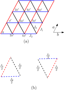
Figure 8: (a) Two-dimensional triangular lattice system containing $J_{1}$(red), $J_{3}$(black) and $J_{2}$(blue) superexchange interaction, with the spiral angle at different sites are shown. (b) Two basic elements of the triangular lattice.

Our method can be applied to the compounds of layers of triangular lattice, such as ACrO₂ To08 (A=Cu, Ag, Li or Na) shown in Fig. 8(a). Here we assume that the exchange interaction $J_{1}$ along $a$-axis,$J_{2}$ along $b$-axis is $J_{2}$ and $J_{3}$ along $\vec{a}-\vec{b}$ axis. For simplicity, we consider the case $J_{3}=J_{1}$, then we have

$$H^{2D}= \sum_{\langle j,k\rangle}J_{1}[\Delta_{1}s_{j,k}^{z}s_{j^{\prime},k}^{z}+\frac{1}{2}(s_{j,k}^{+}s_{j^{\prime},k}^{-}+s_{j,k}^{-}s_{j^{\prime},k}^{+})$$

$$+D_{1}\vec{s}_{j,k}\times\vec{s}_{j^{\prime},k}\cdot\hat{z}]$$

$$+J_{2}[\Delta_{2}s_{j,k}^{z}s_{j,k^{\prime}}^{z}+\frac{1}{2}(s_{j,k}^{+}s_{j,k^{\prime}}^{-}+s_{j,k}^{-}s_{j,k^{\prime}}^{+})$$

$$+D_{2}\vec{s}_{j,k}\times\vec{s}_{j,k^{\prime}}\cdot\hat{z}]]$$ (28)

where $j$ stands for the site index along $b$-direction, and $k$ is the index along $a$-direction. Defining $D_{1}=\tan(\phi_{1}),D_{2}=\tan(\phi_{2})$, and performing a unitary transformation $U(\phi^{\prime})$, we get an isotropic Hamiltonian

$$H_{iso}^{2D}= \sum_{\langle j,k\rangle}J_{1}\Delta_{1}[\vec{s}_{j,k}\cdot\vec{s}_{j^{\prime},k}+D_{1}^{\prime}\vec{s}_{j,k}\times\vec{s}_{j^{\prime},k}\cdot\hat{z}]$$

$$+J_{2}\Delta_{2}[\vec{s}_{j,k}\cdot\vec{s}_{j,k^{\prime}}+D_{2}^{\prime}\vec{s}_{j,k}\times\vec{s}_{j,k^{\prime}}\cdot\hat{z}]$$

with the parameters $\Delta_{1}=\frac{\cos(\phi_{1}-\phi^{\prime})}{\cos(\phi_{1})},\Delta_{2}=\frac{\cos(\phi_{2}-2\phi^{\prime})}{\cos(\phi_{2})}$ and $D_{1}^{\prime}=\tan(\phi_{1}-\phi^{\prime}),D_{2}^{\prime}=\tan(\phi_{2}-2\phi^{\prime})$. For Hamiltonian $H_{iso}^{2D}$ , FP state is the eigen state, and for Hamiltonian $H^{2D}$, spiral state is the eigen state.

The Hamiltonian of a layer is the combination of many local Hamiltonians of small triangles, as shown in Fig. 8(b). For each local Hamiltonian, we can perform our analysis as before. The local site Hamiltonian is the same as that described in 1D zigzag spin chain. Therefore, the region for PSD is the same as that of zigzag spin chain in Eq. (13), and Eq. (10) also applies.

Consider isotropic exchange interaction as an example. We set $\Delta_{1}=\Delta_{2}=1$ and $\phi_{1}=\phi^{\prime}/2,\phi_{2}=\phi^{\prime}$. It was found that the PSD condition gives

$$\phi^{\prime}=\Big{\{}\begin{array}[c]{cc}0^{0}\sim 90^{0},270^{0}\sim 360^{0}&,\mbox{ for }J_{2}>0\\ 90^{0}\sim 270^{0}&,\mbox{ for }J_{2}<0\end{array}$$

Our method has the potential application to two-dimensional spin system.

VI Analysis and discussion

We now compare our results with those of numerical calculations and simulations. The results from the calculations (see below) show that the zigzag spin chain possesses rather rich and sophisticate physics. Since our method is to find the exact solutions, we can only access limited regions in phase space. However, inside these regions, our results are exact and thus can be used as standard to check the results of numerical calculations. Our calculation can also serve as a guideline for the calculation of the correlation functions outside of these regions. Hence, by comparison, we hope to shed some light on the complex physical landscape of the zigzag spin chain.

There are many works on the phase diagram. Hikihara et al. Hik01 used Density matrix renormalization group (DMRG) method and found spin-liquid, dimer and gapless chiral phase for various quantum spins. For $s=1/2$, they found notably, the chiral correlation function $\langle\vec{s}_{j}\times\vec{s}_{j+d}\rangle$, has long-range order behavior. Plekhanov et al.Ple10 also used DMRG technique to study similar systems. They found that quantum fluctuation modified the classical phase diagram. In particular, they found phases denoted by spin liquid I, spin liquid II, E-I and E-II. In the former two phases, they found that the spin correlation functions (especially those on x-y plane $\langle s_{j}^{x}s_{j+d}^{x}\rangle$) have the power-law decay behavior. In the E-I and E-II phases, the spin correlation functions decrease exponentially except for a weak magnetization in E-I phase. Jafari et al.Jaf07 used quantum renormalization group, to find a similar phase diagram except for a new phase near the spin liquid I. It was designated as dimer II. For $J_{1}<0$, the spin liquid III have more or less occupied regions of E-II phase of Plekhanov et al.Ple10 . Dmitriev and Krivnov Dv07 studied the same problem with variational mean-field approximation and scaling. They also obtained similar region of spin-liquid I in the phase diagram. On the other hand, their incommensurate phase (III) fits roughly within the region of E-II phase of Plekhanov.

Since all the above calculation did not consider DM interaction, we set $D_{1}=D_{2}=0$ at beginning in order to make comparison. This, in our calculation, is to set $\Delta_{1}=\cos(\phi^{\prime}),\Delta_{2}=\cos(2\phi^{\prime})$. The exact solution can be found when Eq. (16) is satisfied. We consider the case $J_{2}>0$. The notations of the phase diagram of Dmitriev and Krivnov Dv07 was chosen because their mean field calculation gives clear boundaries between phases. Besides, the result of Plekhanov et al.Ple10 is consistent with that of Dmitriev and Krivnov Dv07 . Our result is shown by the heavy solid line in Fig. 9. The ground states are the spiral spin states with different pitch angles. The exact solution is in the region of incommensurate phase or the E-II phase of ref. 33 or that of spin liquid III of ref. 35. Our calculation shows that on the solid line the one-magnon state is gapless and the chiral correlation has long-range order behavior due to spiral spins. For larger $\Delta_{1}$, numerical calculations, except for ref. 33, found a gapless chiral phase. For smaller $\Delta_{1}$, it has been argued Jaf07 that it is a phase (denoted by spin fluid I) of XXZ model without long-range order. Our calculation also shows that one-magnon modes actually have lower energy than that of spiral spin state as it can be seen from Eq. (19). Hence, it is plausible to assume that the solid curve is the exact boundary of a gapless chiral phase. We noticed that our curve is close to those given in ref. 35 in the region $0.25\leq J=-J_{2}/J_{1}\leq 0.28$ but the difference increases as $J_{2}/J_{1}$ increases. Since the calculation of Dmitriev and Krivnov Dv07 is less accurate for larger $J_{2}/J_{1}$ whereas ours is exact, this discrepancy is expected. Further study is needed to confirm that the curve by our calculation is indeed the phase boundary. A final note of this case is that there exists another “mirror” curve if one makes the transformation: $\Delta_{1}\rightarrow-\Delta_{1},J_{1}\rightarrow-J_{1},\phi^{\prime}\rightarrow\pi-\phi^{\prime}$. This is actually equivalent to rotating the spins of odd sites around z-axis by $\pi$.

Next, we discuss the effect of DM interaction. With DM interaction, the general form of the ratio of the couplings changes from Eq. (16) to the following

$$\frac{J_{1}}{J_{2}}=-2\frac{\sin(\phi_{2}-2\phi^{\prime})}{\sin(\phi_{1}-\phi^{\prime})}\frac{\cos(\phi_{1})}{\cos(\phi_{2})},$$ (29)

as was given in Eq. (10). The system is more apt to have a spiral spin ground state. For example, in Fig. 9, the heavy dashed ($D_{1}=0.1$) and dotted lines ($D_{2}=0.1$) indicate the conditions of such ground states. In these calculations there is a small but non-vanishing $\Delta_{2}$. Fortunately the result of Dmitriev and Krivnov Dv07 shows that the effect of $\Delta_{2}$ will not influence the phase diagram very much. The curves evidence that the spiral spin states can be the ground state in the spin-fluid I phase of ref. 33. In other words, DM interaction makes chiral correlation more robust.

For the case $J_{1}>0$ which was considered by Hikihara et al. Hik01 , if there is no DM interaction, there is no spiral spin ground state. The reason is simple. In view of Eq. (16) $\cos(\phi^{\prime})$ has to be negative for a positive $J_{1}/J_{2}$. This implies that $\Delta_{1}=\cos(\phi^{\prime})<0$, is contradict to our starting point of $J_{1}>0$. But if the DM interaction is present, the spiral spin states can still be the ground state as long as the condition Eq. (29) is satisfied. For example, we can choose $\phi^{\prime 0}$. The region of PSD is shown in Fig.5. We may have many possibilities. Some of them are

$$(1.244,3.50,0,3.73,0.176),\phi_{1}=75^{0}\mbox{ and }\phi_{2}=10^{0}.$$

$$(5.85,1.97,0,1.73,0.176),\phi_{1}=60^{0}\mbox{ and }\phi_{2}=10^{0}.$$

$$(1.28,3.50,0.185,3.73,0.364),\phi_{1}=75^{0}\mbox{ and }\phi_{2}=20^{0}$$

where the parentheses give the values of $(J_{1}/J_{2},\Delta_{1},\Delta_{2},D_{1},D_{2})$. Under these conditions, we have $J_{1}>0,J_{2}>0$. Hence, due to the effect of DM interaction, the spiral spin states can be the ground state in the regions of the spin-fluid phase and dimer phase designated by Hikihara et al. Hik01 even if the magnitude of the DM interaction should not be small.

There have been many numerical calculations on the zigzag spin chain system. However, due to the large number of parameters, and hence, large dimension of phase space, and the different methods of calculation, it is not always clear how physical properties change due to the interplays among these parameters. For example, how the system evolves if $\Delta_{1}\Delta_{2}<0$ but its magnitude increases? A very helpful way is to calculate the correlation functions as it has been done in many works. In many cases, finding exact solutions, albeit in a very limited region can provide more clues. A simple calculation shows that the spiral spin state is able to sustain not only the vector chiral spin order but also the oscillatory spin correlation on the easy-plane

$$\langle\sum_{j}s_{j}^{x}s_{j+d}^{x}\rangle=\frac{N}{8}\sin^{2}(\beta)\cos(\phi^{\prime}),$$

where $\phi^{\prime}$ is the spiral angle and $\beta$ is the cone angle. The correlation should oscillate but not decay. Numerical analysis should be able to find long-range order behavior of the chiral correlation function and the $xy$-plane oscillatory spin correlation function. But there is some difficulty due to the symmetry of the Hilbert space caused by the degenerate ground states as we have discussed in section IV. As it has been mentioned, if the anisotropic exchange interaction can be transformed away then it can be shown that all the FP states are the ground states of the transformed Hamiltonian. This implies that our Hamiltonian has huge degeneracy. The ground state can be any linear combination of these degenerate states. If in numerical calculation, the sample of ground states is not large enough, the symmetry can be lost and correlation functions decay faster than they should be.

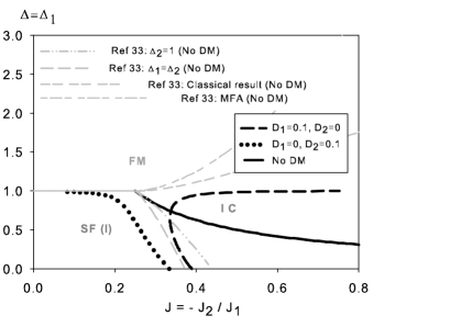
Figure 9: The phase diagram according to ref. 35. Our results are shown in the solid line (no DM interaction), the dashed line ($D_{1}=0.1,D_{2}=0$), and the dotted line ($D_{1}=0,D_{2}=0.1$). SF (I) and IC denote spin-fluid (I) and incommensurate phases.

VII Conclusions

To find the conditions for spiral spin state as the ground state, we transform the physical Hamiltonian to a Hamiltonian with isotropic exchange interaction and DM interaction. The FP states are the eigen states of the transformed Hamiltonian. Then we used positive semi-definite theorem to identify the region of FP state being the GS for the transformed Hamiltonian, which is nothing but the same region of spiral spin state as GS of the original Hamiltonian. The region (shown in Fig. 4) can be expressed by a very simple relation with the couplings of NN and NNN superexchange interaction and DM interaction. The effect of DM interaction is important because its strength is related to the pitch angle of spiral spins and the unitary transformation. As the strength of the DM interaction increases, the pitch angle $\phi^{\prime}$ also increases. It was also found that for spiral spin states to be GS, either $2\phi_{1}=2\tan^{-1}(D_{1})\geq 2\phi_{2}=2\tan^{-1}(D_{2})$ and $\phi_{1}\leq\phi^{\prime}\leq\phi_{2}/2+\pi/4$, or $\phi_{2}/2-\pi/4\leq\phi^{\prime}\leq\phi_{2}/2$ and $\phi^{\prime}\leq\phi_{1}\leq\phi_{2}/2+\pi/2$. Wherever the equal signs stand, the spiral spin states are degenerate with one-magnon states for the physical Hamiltonian in Eq. (1). Hence, the boundary in Fig. 4 marks the region where the spiral spin states being the GS. We thus made manifestly the relation between DM interaction and spiral spin states.

These results can serve as a guided line for experimentalists to find spiral spin state which, in turn, can lead to multiferroics. Our results also show the connection between spiral spins and magnetic frustration. Finally, our method can be applied to other types of magnetic system such as coupled spin chains and layer structure. It is not restricted to spin-$1/2$ system, but can be applied to any spin system.

- (1) Akio Yoshimori, J. Phys. Soc. Jpn. 14 807 (1959).
- (2) T. Nagamiya, K. Nagata and Y. Kitano, Prog. Theo. Phys. 27, 1253 (1962).
- (3) T. Nagamiya, J. de Phys. Rad. 20, 70 (1959).
- (4) K. F. Wang, J. M. Liu and Z. F. Ren, Adv. Phys. 58, 321 (2009).
- (5) M. Kenzelmann, A. B. Harris, S. Jonas, C. Broholm, J. Schefer, S. B. Kim, C. L. Zhang, S.-W. Cheong, O. P. Vajk, and J. W. Lynn, Phys. Rev. Lett. 95, 087206 (2005).
- (6) Y. J. Choi, H. T. Yi, S. Lee, Q. Huan, V. Kiryukhin and S-W. Cheong, Phys. Rev. Lett. 100, 047601(2008) and S. Park, Y. J. Choi, C. L. Zhang and S-W. Cheong, Phys. Rev. Lett. 98, 057601(2008) .
- (7) H. Katsura, N. Nagaosa and A. V. Balatsky, Phys. Rev. Lett. 95, 057205 (2005).
- (8) T. Kimura, Y. Sekio, H. Nakamura, T. Siegrist and A. P. Ramirez, Nat. Mat. 7, 291-294.
- (9) Y. Tokura and S. Seki, Adv. Mater., 21, 1 (2009).
- (10) Masuda, A. Zheludev, A. Bush, M. Markina, and A. Vasiliev, Phys. Rev. Lett. 92, 177201 (2004).
- (11) A. Rusydi, I. Mahns, S. Muller, M. Rubhausen, S. Park, Y. J. Choi, C. L. Zhang, S.-W. Cheong, S. Smadici, P. Abbamonte, M. v. Zimmermann and G. A. Sawatzky, Appl. Phys. Lett. 92, 262506 (2008).
- (12) Yoshiaki Kobayashi, Kenji Sato, Yukio Yasui, Taketo Moyoshi, Masatoshi Sato and Kazuhisa Kakurai, J. Phys. Soc. Jpn. 78, 084721 (2009).
- (13) L. Capogna, M. Reehuis, A. Maljuk, R. K. Kremer, B. Ouladdiaf, M. Jansen, and B. Keimer, Phys. Rev. B 82, 014407 (2010)
- (14) W. Geertsma and D. Khomskii, Phys. Rev. B 54, 3011 (1996).
- (15) S. Seki, Y. Onose and Y. Tokura, Phys. Rev. Lett. 101, 067204 (2008).
- (16) C. K. Majumdar, D. k. Ghosh, J. Math. Phys. 10, 1388 (1969).
- (17) T. Hanada, J. Kane, S. Nakagawa and Y. Natsume, J. Phys. Soc. Japan 57, 1891 (1988) and 58, 3869 (1989).
- (18) R. Bursill, G. A. Gehring, D. J. J. Farnell, J. B. Parkinson, Tao Xiang and Chen Zeng, J. Phys.: Cond. Matt. 7, 8605 (1995).
- (19) S. R. White and I. Affleck, Phys. Rev. B 54, 9862 (1996).
- (20) T. Hikihara, M. Kaburagi, H. Kawamura, arXiv: cond-matt/0010283 (2001).
- (21) I. P. McCulloch, R. Kube, M. Kurz, A. Kleine, U. Schollwock, and A. K. Kolezhuk, Phys. Rev. B 77, 094404 (2008).
- (22) K. Ojunishi, J. Phys. Soc. Jpn. 77, 114004 (2008).
- (23) I. Dzyaloshinskii, J. Phys. Chem. Solids 4, 241 (1958).
- (24) T. Moriya, Phys. Rev. 120, 91 (1960).
- (25) Y. Onose, T. Ideue, H. Katsura, Y. Shiomi, N. Nagaosa and Y. Tokura, Science 329, 297 (2010).
- (26) O. A. Tretiakov and A. Abanov, Phys. Rev. Lett. 105, 157201 (2010).
- (27) I. G. Bostrem, Jun-ichiro Kishine and A. S. Ovchinnikov, Phys. Rev. B 78, 064425 (2008).
- (28) L. Shekhtman, O. Entin-Wohlman, and Amnon Aharony, Phys. Rev. Lett. 69, 836 (1995).
- (29) Meihua Chen, Sujit Sarkar and C. D. Hu, Physica B 406 2211 (2011).
- (30) C. D. Batista, Phys. Rev. B 80, 180406 (2009).
- (31) A. A. Gippius, E. N. Morozova, A. S. Moskvin, A. V. Zalessky, A. A. Bush, M. Baenitz, H. Rosner and S.-L. Drechsler, Phys. Rev. B. 70, 020406 (R) (2004).
- (32) T. Hikihara, M. Kaburagi, and H. Kawamura, Can. J. Phys. 79 1587 (2001) and Phys. Rev. B 63, 174430 (2001).
- (33) E. Plekhanov, A. Avella and F. Mancini, Euro. Phys. J. B - Cond. Mat. 77, 381 (2010).
- (34) R. Jafari, A. Langari, Physica A 364, 213 (2006) and Phys. Rev. B 76, 014412 (2007).
- (35) D. V. Dmitriev and V. Ya. Krivnov, Phys. Rev. B 75, 014424 (2007) and Phys. Rev. B 77, 024401 (2008).