Modified gravity models of dark energy
Abstract
We review recent progress of modified gravity models of dark energy–based on gravity, scalar-tensor theories, braneworld gravity, Galileon gravity, and other theories. In gravity it is possible to design viable models consistent with local gravity constraints under a chameleon mechanism, while satisfying conditions for the cosmological viability. We also construct a class of scalar-tensor dark energy models based on Brans-Dicke theory in the presence of a scalar-field potential with a large coupling strength between the field and non-relativistic matter in the Einstein frame. We study the evolution of matter density perturbations in and Brans-Dicke theories to place observational constraints on model parameters from the power spectra of galaxy clustering and Cosmic Microwave Background (CMB).
The Dvali-Gabadazde-Porrati braneworld model can be compatible with local gravity constraints through a nonlinear field self-interaction arising from a brane-bending mode, but the self-accelerating solution contains a ghost mode in addition to the tension with the combined data analysis of Supernovae Ia (SN Ia) and Baryon Acoustic Oscillations (BAO). The extension of the field self-interaction to more general forms satisfying the Galilean symmetry in the flat space-time allows a possibility to avoid the appearance of ghosts and instabilities, while the late-time cosmic acceleration can be realized by the field kinetic energy. We study observational constraints on such Galileon models by using the data of SN Ia, BAO, and CMB shift parameters.
We also briefly review other modified gravitational models of dark energy–such as those based on Gauss-Bonnet gravity and Lorentz-violating theories.
I Introduction
The cosmic acceleration today has been supported by independent observational data such as the Supernovae-type Ia (SN Ia) Riess ; Perlmutter , the Cosmic Microwave Background (CMB) temperature anisotropies measured by WMAP WMAP1 ; WMAP7 , and Baryon Acoustic Oscillations BAO1 ; BAO2 . The origin of dark energy responsible for this cosmic acceleration is one of the most serious problems in modern cosmology review1 ; review2 ; review3 ; review4 ; reviewSahni ; review5 ; Noreview ; Woodard ; Durrer ; Lobo ; review6 ; Braxreview ; review7 ; review8 . The cosmological constant is one of the simplest candidates for dark energy, but it is plagued by a severe energy scale problem if it originates from the vacuum energy appearing in particle physics Weinberg .
The first step toward understanding the nature of dark energy is to clarify whether it is a simple cosmological constant or it originates from other sources that dynamically change in time. The dynamical models can be distinguished from the cosmological constant by considering the evolution of the equation of state of dark energy (). The scalar field models of dark energy such as quintessence quin1 ; quin2 ; quin3 ; quin4 ; quin5 and k-essence kes1 ; kes2 predict a wide variety of the variation of , but still the current observational data are not sufficient to distinguish those models from the -Cold-Dark-Matter (CDM) model. Moreover it is generally difficult to construct viable scalar-field models in the framework of particle physics because of a very tiny mass ( eV) required for the cosmic acceleration today Carroll98 ; Kolda .
There exists another class of dynamical dark energy models based on the large-distance modification of gravity. The models that belong to this class are gravity fRearly1 ; fRearly2 ; fRearly3 ; fRearly4 ( is function of the Ricci scalar ), scalar-tensor theories stearly1 ; stearly2 ; stearly3 ; stearly4 ; stearly5 ; stearly6 , braneworld models DGP , Galileon gravity Nicolis , Gauss-Bonnet gravity NOS05 ; NO05 , and so on. An attractive feature of these models is that the cosmic acceleration can be realized without recourse to a dark energy matter component. If we modify gravity from General Relativity (GR), however, there are tight constraints coming from local gravity tests as well as a number of observational constraints. Hence the restriction on modified gravity models is in general stringent compared to modified matter models (such as quintessence and k-essence).
For example, an model of the form () was proposed to explain the late-time cosmic acceleration fRearly2 ; fRearly3 (see also Refs. Soussa ; Allem ; Easson ; Dick04 ; Carloni ; Brookfield for early works). However this model suffers from a number of problems such as the incompatibility with local gravity constraints Chiba ; Dolgov ; Olmo ; Navarro , the instability of density perturbations matterper1 ; matterper2 ; SongHu1 ; SongHu2 , and the absence of a matter-dominated epoch APT ; APT2 . As we will see in this review there are a number of conditions required for the viability of dark energy models matterper1 ; matterper2 ; SongHu1 ; SongHu2 ; Teg ; AGPT ; LiBarrow ; AmenTsuji07 ; Fay07 ; Pogosian ; Sendouda , which stimulated to propose viable models Hu07 ; Star07 ; Appleby ; Tsuji08 ; LinderfR .
The simplest version of scalar-tensor theories is so-called Brans-Dicke theory in which a scalar field couples to the Ricci scalar with the Lagrangian density , where is a so-called Brans-Dicke parameter BD . GR can be recovered by taking the limit . If we allow the presence of the field potential in Brans-Dicke theory, theory in the metric formalism is equivalent to this generalized Brans-Dicke theory with the parameter ohanlon ; Chiba . By transforming the action in generalized Brans-Dicke theory (“Jordan frame”) to an “Einstein frame” action by a conformal transformation, the theory in the Einstein frame is equivalent to a coupled quintessence scenario coupled with a constant coupling satisfying the relation TUMTY . For example, theory in the metric formalism corresponds to the constant coupling , i.e. . For of the order of unity it is generally difficult to satisfy local gravity constraints unless some mechanism can be at work to suppress the propagation of the fifth force between the field and non-relativistic matter. It is possible for such large-coupling models to be consistent with local gravity constraints Cembranos ; Teg ; Hu07 ; AmenTsuji07 ; CapoTsuji ; Van ; Gannouji10 through the so-called chameleon mechanism KW1 ; KW2 , provided that a spherically symmetric body has a thin-shell around its surface.
A braneworld model of dark energy was proposed by Dvali, Gabadadze, and Porrati (DGP) by embedding a 3-brane in the 5-dimensional Minkowski bulk spacetime DGP . In this scenario the gravitational leakage to the extra dimension leads to a self-acceleration of the Universe on the 3-brane. Moreover a longitudinal graviton (i.e. a brane-bending mode ) gives rise to a nonlinear self-interaction of the form through the mixing with a transverse graviton, where is a cross-over scale (of the order of the Hubble radius today) and is the Planck mass DGPnon1 ; DGPnon2 . In the local region where the energy density is much larger than the nonlinear self-interaction can lead to the decoupling of the field from matter through the so-called Vainshtein mechanism Vainshtein , which allows a possibility for the consistency with local gravity constraints. However the DGP model suffers from a ghost problem DGPghost1 ; DGPghost2 ; DGPghost3 , in addition to the difficulty for satisfying the combined observational constraints of SN Ia and BAO DGPobser1 ; DGPobser2 ; DGPobser3 ; DGPobser4 ; DGPobser5 ; DGPobser6 .
The equations of motion following from the self-interacting Lagrangian present in the DGP model are invariant under the Galilean shift in the Minkowski background. While the DGP model is plagued by the ghost problem, the extension of the field self-interaction to more general forms satisfying the Galilean symmetry may allow us to avoid the appearance of ghosts. Nicolis et al. Nicolis showed that there are only five field Lagrangians () that respect the Galilean symmetry in the Minkowski background. In Refs. Deffayetga1 ; Deffayetga2 these terms were extended to covariant forms in the curved space-time. In addition one can keep the equations of motion up to the second-order, while recovering the Galileon Lagrangian in the limit of the Minkowski space-time. This property is welcome to avoid the appearance of an extra degree of freedom associated with ghosts. In fact, Refs. DT2 ; DT3 derived the viable model parameter space in which the appearance of ghosts and instabilities associated with scalar and tensor perturbations can be avoided. Moreover the late-time cosmic acceleration is realized by the existence of a stable de Sitter solution. We shall review the cosmological dynamics of Galileon gravity as well as conditions for the avoidance of ghosts and instabilities.
In order to distinguish between different models of dark energy based on modified gravitational theories, it is important to study the evolution of cosmological perturbations as well as the background expansion history of the Universe. In particular, the modified growth of matter perturbations relative to the CDM model changes the matter power spectrum of large-scale structures (LSS) as well as the weak lensing spectrum obsermo1 -Song10 . Moreover the modification of gravity manifests itself for the evolution of the effective gravitational potential related with the Integrated-Sachs-Wolfe (ISW) effect in CMB anisotropies. We shall review a number of observational signatures for the modified gravitational models of dark energy.
This review is organized as follows. In Sec. II we construct viable dark energy models based on theories after discussing conditions for the cosmological viability as well as for the consistency with local gravity tests. In Sec. III we show that, in Brans-Dicke theories with large matter couplings, it is possible to design the field potential consistent with both cosmological and local gravity constraints. In Sec. IV we derive the field equations in the DGP model and confront the model with observations at the background level. In Sec. V we review the cosmological dynamics based on Galileon gravity as well as conditions for the avoidance of ghosts and Laplacian instabilities. In Sec. VI we briefly mention other modified gravity models of dark energy based on Gauss-Bonnet gravity and Lorentz-violating theories. In Sec. VII we study observational signatures of dark energy models based on gravity, Brans-Dicke theory, DGP model, and Galileon gravity, in order to confront them with the observations of LSS, CMB, and weak lensing. Sec. VIII is devoted to conclusions.
Throughout the review we use the units such that , where is the speed of light, is reduced Planck’s constant, and is Boltzmann’s constant. We also adopt the metric signature .
II gravity
We start with the action in gravity:
| (1) |
where ( is a bare gravitational constant), is a determinant of the metric , is an arbitrary function in terms of the Ricci scalar , and is a matter action with matter fields . Variation of the action (1) with respect to leads to the following field equation
| (2) |
where , is a Ricci tensor, and is an energy-momentum tensor of matter. The trace of Eq. (2) gives
| (3) |
where . Here and are the energy density and the pressure of matter, respectively.
Regarding the variation of the action (1), there is another approach called the Palatini formalism Palatini1919 in which and the affine connection are treated as independent variables.111We also note that there is another approach for the variational principle–known as the metric-affine formalism–in which the matter Lagrangian depends not only on the metric but also on the connection Hehl ; Liberati ; Liberati2 ; Capome . The resulting field equations are second-order Ferraris ; Vollick ; Vollick2 ; Flanagan0 ; Flanagan ; Flanagan2 and the cosmological dynamics of dark energy models have been studied by a number of authors Meng ; Meng2 ; Meng3 ; NOpala ; Sot ; Sotinf ; Motapala ; FayTavakol . However theory in the Palatini formalism gives rise to a large coupling between a scalar field degree of freedom and ordinary matter Flanagan0 ; Flanagan ; Flanagan2 ; Kaloper ; OlmoPRL2 ; Olmo08 ; Olmo09 ; Barausse1 , which implies difficulty for compatibility with standard models of particle physics. This large coupling also leads to significant growth of matter density perturbations, unless the models are very close to the CDM model KoivistoPala ; KoivistoPala2 ; LiPala0 ; LiPala ; TsujiUddin .
In the following we focus on the variational approach (so called the metric formalism) given above. The Einstein gravity without a cosmological constant corresponds to and , so that the term in Eq. (3) vanishes. Since in this case , the Ricci scalar is directly determined by matter. In gravity with a non-linear term in , does not vanish in Eq. (3). Hence there is a propagating scalar degree of freedom, , dubbed “scalaron” in Ref. Star80 . The trace equation (3) allows the dynamics of the scalar field .
The de Sitter point corresponds to a vacuum solution with constant . Since at this point, we obtain
| (4) |
Since the quadratic model satisfies this condition, it gives rise to an exact de Sitter solution. In the inflation model proposed by Starobinsky Star80 , the accelerated cosmic expansion ends when the term becomes smaller than the linear term . It is possible to construct such inflation models in the framework of supergravity Ketov1 ; Ketov2 .
II.1 Cosmological dynamics in gravity
We first study cosmological dynamics for the models based on theories in the metric formalism. In order to derive conditions for the cosmological viability of models we shall carry out general analysis without specifying the form of . We consider a flat Friedmann-Lematre-Robertson-Walker (FLRW) background with the line element
| (5) |
where is a scale factor. For the matter Lagrangian in Eq. (1) we take into account non-relativistic matter and radiation, whose energy densities and satisfy the usual continuity equations and respectively. Here is the Hubble parameter and a dot represents a derivative with respect to cosmic time . From Eqs. (2) and (3) we obtain
| (6) | |||||
| (7) |
where the Ricci scalar is given by
| (8) |
Let us introduce the following dimensionless variables:
| (9) |
together with the density parameters
| (10) |
It is straightforward to derive the following equations AGPT :
| (11) | |||||
| (12) | |||||
| (13) | |||||
| (14) |
where and
| (15) | |||||
| (16) |
From Eq. (16) one can express as a function of . Since is a function of , it follows that is a function of , i.e., . The CDM model, , corresponds to . Then the quantity characterizes the deviation from the CDM model.
The effective equation of state of the system is given by
| (17) |
In the absence of radiation () the fixed points for the dynamical system (11)-(14) are
| (18) | |||
| (19) | |||
| (20) | |||
| (21) | |||
| (22) | |||
| (23) |
The points and are on the line in the plane.
Only the point can be responsible for the matter-dominated epoch ( and ). This is realized provided is close to 0. In the () plane the matter point exists around . Either the point or can lead to the late-time cosmic acceleration. The former corresponds to a de Sitter point () with , in which case the condition (4) is satisfied. Depending on the values of , the point can be responsible for the cosmic acceleration AGPT . In the following we shall focus on the case in which the matter point is followed by the de Sitter point .
The stability of the fixed points is known by considering small perturbations () around them AGPT . For the point the eigenvalues for the Jacobian matrix of perturbations are
| (24) |
where and with . In the limit the latter two eigenvalues reduce to . The models with show a divergence of the eigenvalues as , in which case the system cannot remain for a long time around the point . For example the model with and falls into this category. On the other hand, if , the latter two eigenvalues in Eq. (24) are complex with negative real parts. Then, provided that , the point corresponds to a saddle point with a damped oscillation. Hence the Universe can evolve toward the point from the radiation era and leave for the late-time acceleration. Then the condition for the existence of the saddle matter era is
| (25) |
The first condition implies that the models need to be close to the CDM model during the matter era.
The eigenvalues for the Jacobian matrix of perturbations about the point are
| (26) |
where . This shows that the condition for the stability of the de Sitter point is Muller ; Faraonista1 ; Faraonista2 ; AGPT
| (27) |
The trajectories that start from the saddle matter point with the condition (25) and then approach the stable de Sitter point with the condition (27) are cosmologically viable.
Let us consider a couple of viable models in the plane. The CDM model, , corresponds to , in which case the trajectory is a straight line from : to : . The trajectory (ii) in Fig. 1 represents the model AmenTsuji07 , which corresponds to the straight line in the plane. The existence of a saddle matter epoch requires the condition and . The trajectory (iii) represents the model AGPT ; LiBarrow
| (28) |
which corresponds to the curve . The trajectory (iv) in Fig. 1 shows the model , in which case the late-time accelerated attractor is the point with .

In Ref. AGPT it was shown that the variable needs to be close to 0 during the radiation-dominated epoch as well. Hence the viable models are close to the CDM model, , in the region (where is the present cosmological Ricci scalar). The Ricci scalar given in Eq. (8) remains positive from the radiation era to the present epoch, as long as the it does not oscillate. As we will see in Sec. II.2, we require the condition to avoid ghosts. Then the condition for the presence of the matter-dominated epoch translates to . The model (, ) is not viable because the condition is violated. We also note that the power-law models with do not give rise to a successful cosmological trajectory APT ; APT2 (unlike the claims in Ref. CNOT ).
In order to derive the equation of state of dark energy to confront with SN Ia observations for the cosmologically viable models, we rewrite Eqs. (6) and (7) as follows222If the field equations are written in this form, we can also show that the background cosmological dynamics has a correspondence with equilibrium thermodynamics on the apparent horizon BGT09 .:
| (29) | |||
| (30) |
where is some constant and
| (31) | |||||
| (32) |
Defining and in this way, one can show that these satisfy the usual continuity equation
| (33) |
The dark energy equation of state related with SN Ia observations is given by . From Eqs. (29) and (30) it follows that
| (34) |
where the last approximate equality in Eq. (34) is valid in the regime where the radiation density is negligible relative to the matter density. The viable models approach the CDM model in the past, i.e. as . In order to reproduce the standard matter era for the redshifts , one can choose in Eqs. (29) and (30). Another possible choice is , where is the present value of . This choice is suitable if the deviation of from 1 is small (as in the scalar-tensor theory with a massless scalar field Torres ; Boi00 ; Espo ). In both cases the equation of state can be smaller than before reaching the de Sitter attractor AmenTsuji07 ; Tsuji08 ; Motohashi10 ; Bamba10 ; Bamba10d . Thus gravity models give rise to a phantom equation of state without violating stability conditions of the system.
As we see in Eq. (34), the presence of non-relativistic matter is important to lead to the apparent phantom behavior. We wish to stress here that for viable models constructed to satisfy all required conditions [such as the models (45), (46), and (48) we will discuss later] the ghosts are not present even if . A number of authors proposed some models to realize without including non-relativistic matter Bamba08 ; Bamba09 , which means that from Eq. (34). However, such models usually imply the presence of ghosts333If a late-time de Sitter solution is a stable spiral, it happens that oscillates around with a small amplitude, even for viable models. Here we are discussing the real ghosts out of this regime., because corresponds to .
The observational constraints on specific models have been carried out in Refs. Dev ; Mel09 ; Cardone09 ; Ali10 from the background expansion history of the Universe (see also Refs. Caporecon ; Mul06 ; Dobado06 ; Wu07 ; Carloni10 for the reconstruction of models from observations). Since the deviation of from that in the CDM model () is not so significant Hu07 ; Motohashi10 , the viable models such as (45), (46), and (48) can be consistent with the data fairly easily. In other words we do not obtain very tight bounds on model parameters from the information of the background expansion history only. However, the models can be more strongly constrained at the level of perturbations, as we will see in Sec. VII.1.
II.2 Conditions for the avoidance of ghosts and tachyonic instabilities
In this subsection we shall derive conditions for the avoidance of ghosts and tachyonic instabilities in theories. In doing so we expand the action (1) up to the second-order by considering the following perturbed metric about the FLRW background
| (35) |
where are scalar metric perturbations Bardeen .
Introducing the perturbation for the quantity , one can construct the gauge-invariant curvature perturbation
| (36) |
Expanding the action (1) without the matter source, we obtain the second-order action for the curvature perturbation Hwang97 ; review7
| (37) |
where
| (38) |
The negative sign of corresponds to a ghost field because of the negative kinetic energy. Hence the condition for the avoidance of ghosts is given by
| (39) |
For the matter sector the ghost does not appear for (where is the equation of state for the matter fluid) DMT , which is satisfied for radiation () and non-relativistic matter ().
If is positive, the action (37) can be written in the following form by introducing the new variables and :
| (40) |
where a prime represents a derivative with respect to the conformal time . Equation (40) shows that the scalar degree of freedom has the effective mass
| (41) | |||||
where we have eliminated the term by using the background equations.
In Fourier space the perturbation satisfies the equation of motion
| (42) |
For , the propagation speed of the field is equivalent to the speed of light . Hence, in gravity, the gradient instability associated with negative is absent. For small satisfying , we require that to avoid the tachyonic instability of perturbations. The viable dark energy models based on theories need to satisfy the condition (i.e. ) at early cosmological epochs in order to have successful cosmological evolution from radiation domination till matter domination. At these epochs the mass squared is approximately given by
| (43) |
Under the no-ghost condition (39) the tachyonic instability is absent for
| (44) |
The viable dark energy models have been constructed to satisfy the conditions (39) and (44) in the regime , where is the Ricci scalar at the late-time de Sitter point. Moreover we require that the models are consistent with the conditions (25) and (27). The model (28) can be consistent with all these conditions, but the local gravity constraints demand that the variable is very much smaller than 1 in the regions of high density (i.e. , where is the cosmological Ricci scalar today). In the model (28) one has around . For the consistency with local gravity constraints we require that CapoTsuji , but in this case the deviation from the CDM model around the present epoch () is very small.
If the variable behaves as with in the region , then it is possible to satisfy local gravity constraints (i.e. for ) while at the same time showing deviations from the CDM ( for ). The models constructed in this vein are
| (45) | |||
| (46) |
which were proposed by Hu and Sawicki Hu07 and Starobinsky Star07 , respectively. is roughly of the order of the present cosmological Ricci scalar for and of the order of unity. The models (A) and (B) asymptotically behave as
| (47) |
which gives .
Another viable model that leads to the even rapid decrease of toward the past is Tsuji08
| (48) |
Other similar models were proposed by Appleby and Battye Appleby and Linder LinderfR .
In what follows we shall discuss local gravity constraints on the above models.
II.3 Local gravity constraints on gravity models
Let us proceed to discuss local gravity constraints on gravity models. In the region of high density like Earth or Sun, the Ricci scalar is much larger than the background cosmological value . In this case the linear expansion of cannot be justified. In such a non-linear regime the chameleon mechanism KW1 ; KW2 plays an important role for the models to satisfy local gravity constraints Cembranos ; Teg ; Hu07 ; AmenTsuji07 ; CapoTsuji ; Van ; Gannouji10 (see also Refs. OlmoPRL ; Olmo05 ; Fara06 ; Erick06 ; Chiba07 ; Kainu07 ; Kainu08 ).
To discuss the chameleon mechanism in gravity, it is convenient to transform the action (1) to the so-called Einstein frame action via the conformal transformation Maeda :
| (49) |
The action in the Einstein frame includes a linear term in , where the tilde represents quantities in the Einstein frame. Introducing a new scalar field , we obtain the action in the Einstein frame, as Maeda ; review7
| (50) |
where
| (51) |
In the Einstein frame the scalar field directly couples with non-relativistic matter. The strength of this coupling depends on the conformal factor . We define the coupling as
| (52) |
which is of the order of unity in gravity. If the field potential is absent, the field propagates freely with a large coupling . Since a potential (51) with a gravitational origin is present in gravity, it is possible for dark energy models to satisfy local gravity constraints through the chameleon mechanism Teg ; Hu07 ; CapoTsuji ; Van .
In a spherically symmetric space-time under a weak gravitational background (i.e. neglecting the backreaction of gravitational potentials), variation of the action (50) with respect to the scalar field leads to
| (53) |
where is a distance from the center of symmetry, and is an effective potential defined by
| (54) |
Here is a conserved quantity in the Einstein frame, which is related to the density in the Jordan frame via the relation . By the end of this section we use the unit .
We assume that a spherically symmetric body has a constant density inside the body () and that the density outside the body () is . The mass of the body and the gravitational potential at the radius are given by and , respectively. The effective potential has two minima at the field values and satisfying and , respectively (here a prime represents a derivative with respect to ). The former corresponds to the region with a high density that gives rise to a large mass squared , whereas the latter to the lower density region with a smaller mass squared . When the “dynamics” of the field with the field equation (53) is studied, we need to consider the effective potential so that it has two maxima at and .
We impose the two boundary conditions and . The field is at rest at and begins to roll down the potential when the matter-coupling term becomes important at a radius in Eq. (53). As long as is close to such that , the body has a thin-shell inside the body. The field acquires a sufficient kinetic energy in the thin-shell regime () and hence the field climbs up the potential hill outside the body ().
The field profile can be obtained by matching the solutions of Eq. (53) at the radius and . Neglecting the mass term , the thin-shell field profile outside the body is given by TT08
| (55) |
where
| (56) |
Here is called a thin-shell parameter. Under the conditions and , the thin-shell parameter is approximately given by TT08
| (57) |
Provided that , the amplitude of the effective coupling can be much smaller than 1. It is then possible for the models () to be consistent with local gravity experiments. Originally the thin-shell solution was derived by assuming that the field is frozen in the region KW1 ; KW2 . In this case the thin-shell parameter is given by , which is different from Eq. (57). However, this difference is not important because the condition is satisfied for most of viable models TT08 .
Consider the bound on the thin-shell parameter from the possible violation of equivalence principle (EP). The tightest bound comes from the solar system tests of weak EP using the free-fall acceleration of Moon () and Earth () toward Sun KW2 . The experimental bound on the difference of two accelerations is given by Will05
| (58) |
Provided that Earth, Sun, and Moon have thin-shells, the field profiles outside the bodies are given by Eq. (55) with the replacement of corresponding quantities. The acceleration induced by a fifth force with the field profile and the effective coupling is . Using the thin-shell parameter for Earth, the accelerations and toward Sun (mass ) are
| (59) |
where , , and are the gravitational potentials of Sun, Earth and Moon, respectively. Then the condition (58) translates to
| (60) |
Since the condition is satisfied for viable models (as we will see below), we have from Eq. (56). Hence the condition (60) corresponds to
| (61) |
Let us consider local gravity constraints on the models given in Eqs. (45) and (46). In the region of high density where local gravity experiments are carried out, it is sufficient to use the asymptotic form given in Eq. (47). In order for these models to be responsible for the present cosmic acceleration, is roughly the same order as the cosmological Ricci scalar today for and of the order of unity. For the functional form (47) we have the following relations
| (62) | |||||
| (63) |
Inside and outside the body the effective potential (63) has minima at
| (64) |
If , then one has .
The bound (61) translates into
| (65) |
Here is defined by , where is the Ricci scalar at the late-time de Sitter fixed point given in Eq. (18). Let us consider the model described by the Lagrangian density (47) for . If we use the models (45) and (46), then there are some modifications for the estimation of . However this change is not significant when we place constraints on model parameters.
The de Sitter solution for the model (47) satisfies . Substituting this relation into Eq. (65), it follows that
| (66) |
For the stability of the de Sitter point we require that , which translates into the condition . Hence the term in Eq. (66) is smaller than 0.25 for .
Let us use the simple approximation that and are of the orders of the present cosmological density g/cm3 and the baryonic/dark matter density g/cm3 in our galaxy, respectively. From Eq. (66) we obtain the constraint CapoTsuji
| (67) |
Thus is not required to be much larger than unity. Under the condition (67), as decreases to the order of , one can cosmologically see an appreciable deviation from the CDM model. The deviation from the CDM model appears when decreases to the order of . The model (48) also shows similar behavior. If we consider the model (28), it was shown in Ref. CapoTsuji that the bound (61) gives the constraint . Hence the deviation from the CDM model is very small. The models (45) and (46) are carefully constructed to satisfy local gravity constraints, while at the same time the deviation from the CDM model appears even for . Note that the model (48) can easily satisfy local gravity constraints because of the rapid approach to the CDM in the regime .
In the strong gravitational background (such as neutron stars), Kobayashi and Maeda KM1 ; KM2 pointed out that for the model (46) it is difficult to obtain thin-shell solutions inside a spherically symmetric body with constant density. For chameleon models with general couplings , a thin-shell field profile was analytically derived in Ref. TTT by employing a linear expansion in terms of the gravitational potential at the surface of a compact object with constant density. Using the boundary condition set by analytic solutions, Ref. TTT also numerically confirmed the existence of thin-shell solutions for in the case of inverse power-law potentials . Ref. Upadhye also showed that static relativistic stars with constant density exists for the model (46). The effect of the relativistic pressure is important around the center of the body, so that the field tends to roll down the potential quickly unless the boundary condition is carefully chosen. Realistic stars have densities that globally decrease as a function of . The numerical simulation of Refs. Babi1 ; Babi2 showed that thin-shell solutions are present for the model (46) by considering a polytropic equation of state even in the strong gravitational background (see also Ref. Cooney ).
III Scalar-tensor gravity
There is another class of modified gravity called scalar-tensor theories in which the Ricci scalar is coupled to a scalar field . One of the simplest examples is the so-called Brans-Dicke theory with the action
| (68) |
where is a constant (called the Brans-Dicke parameter), is a field potential, and is a matter Lagrangian that depends on the metric and matter fields . The original Brans-Dicke theory BD does not have the field potential. As we will see below, metric gravity discussed in Sec. II is equivalent to the Brans-Dicke theory with .
III.1 Scalar-tensor theories and the matter coupling in the Einstein frame
The general action for scalar-tensor theories can be written as
| (69) |
where depends on the scalar field and the Ricci scalar , is a function of . We choose the unit . The action (69) covers a wide variety of theories such as gravity (, ), Brans-Dicke theory ( and ), and dilaton gravity ( and ).
Let us consider theories of the type
| (70) |
In order to avoid the appearance of ghosts we require that . Under the conformal transformation (49) with the conformal factor , the action (69) can be transformed to that in the Einstein frame:
| (71) |
where
| (72) |
We have introduced a new scalar field in order to make the kinetic term canonical:
| (73) |
We define the coupling between dark energy and non-relativistic matter in the Einstein frame:
| (74) |
Recall that in metric gravity we have that . If is a constant, the following relations hold from Eqs. (73) and (74):
| (75) |
Then the action (69) in the Jordan frame can be written as TUMTY
| (76) |
In the limit that , the action (76) reduces to the one for a minimally coupled scalar field with the potential . The transformation of the Jordan frame action (76) via a conformal transformation gives rise to the Einstein frame action (71) with a constant coupling . The action (71) is equivalent to the action (50) with .
One can compare (76) with the action (68) in Brans-Dicke theory. Setting , one finds that two actions are equivalent if the parameter is related to via the relation KW2 ; TUMTY
| (77) |
Using this relation, we find that the General Relativistic limit () corresponds to the vanishing coupling (). Since in metric gravity, this corresponds to the Brans-Dicke parameter ohanlon ; Chiba . The experimental bound on for a massless scalar field is given by Will05 ; Iess , which translates into the condition
| (78) |
In such cases it is difficult to find a large difference relative to the uncoupled quintessence model. In the presence of the field potential, however, it is possible for large coupling models () to satisfy local gravity constraints via the chameleon mechanism TUMTY .
The above Brans-Dicke theory is one of the examples in scalar-tensor theories. In general the coupling is field-dependent apart from Brans-Dicke theory. If we consider a nonminimally coupled scalar field with and , then it follows that . The cosmological dynamics in such a theory have been studied by a number of authors stearly1 ; stearly2 ; stearly3 ; stearly4 ; stearly5 ; stearly6 ; Peri1 ; Gannouji06 ; Peri2 ; Martin ; Gunzig ; Verde ; Agarwal ; Jarv ; Leach . If the field is nearly massless during most of the cosmological epochs, the coupling needs to be suppressed to avoid the propagation of the fifth force.
In the following we shall study the cosmological dynamics and local gravity constraints on the constant coupling models based on the action (76) with .
III.2 Cosmological dynamics in Brans-Dicke theory
We study the cosmological dynamics for the Jordan frame action (76) in the presence of a non-relativistic fluid with energy density and a radiation fluid with energy density . We regard the Jordan frame as a physical frame due to the usual conservation of non-relativistic matter (). In the flat FLRW background variation of the action (76) with respect to and gives the following equations of motion
| (79) | |||
| (80) | |||
| (81) |
Let us introduce the following variables
| (82) |
and
| (83) |
These satisfy the relation from Eq. (79). Using Eqs. (79)-(81), we obtain the differential equations for , and :
| (84) | |||||
| (85) | |||||
| (86) |
where , , and
| (87) |
The effective equation of state of the system is given by by .
If is a constant, one can derive the fixed points of the system (84)-(86) in the absence of radiation () TUMTY :
-
•
(a)
(88) -
•
(b)
(89) -
•
(c)
(90) -
•
(d)
(91) -
•
(e)
(92)
The point (e) corresponds to the de Sitter point, which exists only for [this can be confirmed by setting in Eqs. (79)-(81)].
We first study the case of non-zero values of with constant , i.e. for the exponential potential . We do not consider the special case of . The matter-dominated era can be realized either by the point (a) or by the point (d). If the point (a) is responsible for the matter era, the condition is required. We then have and . When the scalar-field dominated point (c) yields an accelerated expansion of the Universe provided that . Under these conditions the point (a) is followed by the late-time cosmic acceleration. The scaling solution (d) can give rise to the equation of state, for . In this case, however, the condition for the point (c) gives . Then the energy fraction of the pressureless matter for the point (d) does not satisfy the condition . From the above discussion the viable cosmological trajectory for constant corresponds to the sequence from the point (a) to the scalar-field dominated point (c) under the conditions and .
We shall proceed to the case where varies with time. The fixed points derived above for constant can be regarded as the “instantaneous” fixed points, provided that the time scale of the variation of is smaller than that of the cosmic expansion. The matter era can be realized by the point (d) with . The solutions finally approach either the de Sitter point (e) with or the accelerated point (c).
In the following we focus on the case in which the matter era with the point (d) is followed by the accelerated epoch with the de Sitter solution (e). To study the stability of the point (e) we define a variable , satisfying the following equation
| (93) |
Considering the matrix for perturbations , and around the point (e), we obtain the eigenvalues
| (94) |
where is the value of at the de Sitter point with the field value . Since , we find that the de Sitter point is stable under the condition
| (95) |
Let us consider the model (47) in which the models (45) and (46) are recovered in the regime . Since , the potential is given by
| (96) |
In this case the slope of the potential, , is
| (97) |
In the deep matter-dominated epoch during which the condition is satisfied, the field is very close to zero. For and of the order of unity, we have at this stage. Hence the matter era can be realized by the instantaneous fixed point (d). As gets smaller, decreases to the order of unity. If the solutions reach the point and satisfy the stability condition , then the final attractor corresponds to the de Sitter fixed point (e).
For the theories with general couplings , it is possible to construct a scalar-field potential that is the generalization of (51). One example is TUMTY
| (98) |
The model (47) corresponds to and . The slope of the potential is given by
| (99) |
We have for and in the limits (for ) and (for ).
The field is nearly frozen around the value during the deep radiation and matter epochs. In these epochs we have from Eqs. (79)-(81) by noting that is negligibly small compared to or . Using Eq. (81), it follows that . Hence, in the high-curvature region, the field evolves along the instantaneous minima given by
| (100) |
The field value increases for decreasing . As long as the condition is satisfied, we have from Eq. (100).
For field values around one has from Eq. (99). Hence the instantaneous fixed point (d) can be responsible for the matter-dominated epoch provided that . The variable decreases in time irrespective of the sign of the coupling and hence . The de Sitter solution corresponds to , that is
| (101) |
This solution is present as long as the solution of this equation exists in the region .
From Eq. (99) the derivative of with respect to is
| (102) |
The de Sitter point is stable under the condition . Using Eq. (101) this translates into
| (103) |
When one can show that is always satisfied. Hence the solutions approach the de Sitter attractor after the end of the matter era. When , the de Sitter point is stable under the condition (103). If this condition is violated, the solutions choose another stable fixed point [such as the point (c)] as an attractor.

The above discussion shows that, if , the matter point (d) can be followed by the stable de Sitter solution (e). In Fig. 2 we plot the evolution of , , , and for , and . This shows that the viable cosmological trajectory can be realized for the potential (98). In order to confront with SN Ia observations, it is possible to rewrite Eqs. (79) and (80) in the forms of Eqs. (29) and (30) by defining the dark energy density and the pressure in the similar way. It was shown in Ref. TUMTY that the phantom equation of state as well as the cosmological constant boundary crossing can be realized for the field potentials satisfying local gravity constraints.
III.3 Local gravity constraints on Brans-Dicke theory
We study local gravity constraints on Brans-Dicke theory described by the action (76). In the absence of the potential we already mentioned that the Brans-Dicke parameter is constrained to be from solar-system experiments. This gives the upper bound (78) on the coupling between the field and non-relativistic matter in the Einstein frame. This bound also applies to the case of a nearly massless field with the potential in which the Yukawa correction is close to unity (where is the scalar field mass and is an interaction length).
In the presence of the field-potential it is possible for large coupling models () to satisfy local gravity constraints provided that the mass of the field is sufficiently large in the region of high density. In fact, the potential (98) is designed to have a large mass in the high-density region, so that it can be compatible with experimental tests of gravity through the chameleon mechanism. In the following we study the model (98) and derive the conditions under which local gravity constraints can be satisfied. If we make a conformal transformation for the action (98), the action in the Einstein frame is given by (76) with . We can use the results obtained in Sec. II.3, because thin-shell solutions have been derived for the general coupling .
As in the case of gravity, we consider a configuration in which a spherically symmetric body has a constant density inside the body and that the density outside the body is given by . Under the condition , we have for the potential in the Einstein frame. Then the field values at the potential minima inside and outside the body are
| (104) |
In order to realize the accelerated expansion today, the energy scale is required to be the same order as the square of the present Hubble parameter , i.e. , where g/cm3 is the cosmological density today. The baryonic/dark matter density in our galaxy corresponds to g/cm3. Hence the conditions and are in fact satisfied unless . The field mass squared at is approximately given by
| (105) |
which means that can be much larger than because of the condition . This large mass allows the chameleon mechanism to work, because the condition is satisfied.
The bound (61) coming from the violation of equivalence principle in the solar system translates into
| (106) |
Let us consider the case in which the solutions finally approach the de Sitter solution (e). At the point (e), one has with given in Eq. (101). Hence we get the following relation
| (107) |
Plugging this into Eq. (106), it follows that
| (108) |
where is the Ricci scalar at the de Sitter point. Since the term is smaller than 1/2 from the condition (103), we obtain the inequality . Using the values g/cm3 and g/cm3, we obtain the following bound
| (109) |
When and we have and , respectively. Thus the model can be compatible with local gravity experiments even for .
In Ref. Gannouji10 it was shown that in order to satisfy both local gravity and cosmological constraints the chameleon potentials in the Einstein frame need to be of the form , where the function is smaller than 1 today and is a mass that corresponds to the dark energy scale ( GeV). The potential KW2 ; Braxchame is one of those viable candidates, but the allowed model parameter space is severely constrained by the 2006 Eöt-Wash experiment Kapner:2006si . Unless the parameter is unnaturally small (), this potential is incompatible with local gravity constraints for .
On the other hand, the chameleon potential () can satisfy both local gravity and cosmological constraints444In the Einstein frame the potential (98) takes the form , so in the region this potential is similar to .. In Ref. Gannouji10 this potential is consistent with the constraint coming from 2006 Eöt-Wash experiments as well as the WMAP bound on the variation of the field-dependent mass Nagata for natural model parameters.
IV DGP model
In this section we review braneworld models of dark energy motivated by string theory. In braneworlds standard model particles are confined on a 3-dimensional (3D) brane embedded in 5-dimensional bulk with large extra dimensions Randall1 ; Randall2 . Dvali, Gabadadze, and Porrati (DGP) DGP proposed a braneworld model in which the 3-brane is embedded in a Minkowski bulk with infinitely large extra dimensions. One can recover Newton’s law by adding a 4D Einstein-Hilbert action sourced by the brane curvature to the 5D action DGP2 . The presence of such a 4D term may be induced by quantum corrections coming from the bulk gravity and its coupling with matter on the brane. In the DGP model the standard 4D gravity is recovered at small distances, whereas the effect from the 5D gravity manifests itself for large distances. Interestingly one can realize the self cosmic acceleration without introducing a dark energy component Deffayet1 ; Deffayet2 (see also Ref. Shtanov ).
IV.1 Self-accelerating solution
The action of the DGP model is given by
| (110) |
where is the metric in the 5D bulk and is the induced metric on the brane with being the coordinates of an event on the brane labelled by . The 5D and 4D gravitational constants, and , are related with the 5D and 4D Planck masses, and , via
| (111) |
The first and second terms in Eq. (110) correspond to Einstein-Hilbert actions in the 5D bulk and on the brane, respectively. There is no contribution to the Lagrangian from the bulk because we are considering a Minkowski bulk. Then the matter action consists of a brane-localized matter whose action is given by , where is the 3-brane tension and is the Lagrangian density on the brane. Since the tension is unrelated to the Ricci scalar , it can be adjusted to be zero (as we do in the following).
In order to study the cosmological dynamics on the brane (located at ), we take a metric of the form:
| (112) |
where represents a maximally symmetric space-time with a constant curvature . The 5D Einstein equations are
| (113) |
where is the 5D Ricci tensor, is the sum of the energy momentum tensor on the brane and the contribution coming from the scalar curvature of the brane:
| (114) |
Since we are considering a homogeneous and isotropic Universe on the brane, one can write in the form
| (115) |
where and are functions of only. The non-vanishing components coming from the Ricci scalar of the brane are
| (116) | |||
| (117) |
where a dot represents a derivative with respect to . The non-vanishing components of the 5D Einstein tensor are Langlois1 ; Langlois2 ; Deffayet1
| (118) | |||
| (119) | |||
| (120) | |||
| (121) |
where a prime represents a derivative with respect to .
Assuming no flow of matter along the 5-th dimensions, we have and hence . Then Eqs. (118) and (121) can be written as
| (122) |
where
| (123) |
Since we are considering the Minkowski bulk, we have and locally in the bulk. This gives and . Integrations of these equations lead to
| (124) |
where is a constant independent of and .
We shall find solutions of the Einstein equations (113) in the vicinity of . The metric needs to be continuous across the brane in order to have a well-defined geometry. However, its derivatives with respect to can be discontinuous at . The Einstein tensor is made of the metric up to the second derivatives with respect to , so the Einstein equations with a distributional source are written in the form Langlois1 ; Langlois2 ; Deffayet1
| (125) |
where is a Dirac’s delta function. Integrating this equation across the brane gives
| (126) |
The jump of the first derivative of the metric is equivalent to the energy-momentum tensor on the brane.
Equations (118) and (119) include the derivatives and of the metric. Integrating the Einstein equations and across the brane, we obtain
| (127) | |||
| (128) |
where the subscript “” represents the quantities on the brane.
We assume the symmetry , in which case and . Substituting Eq. (127) into Eq. (124), we obtain the modified Friedmann equation on the brane:
| (129) |
where is the Hubble parameter and is the sign of . The constant can be interpreted as the term coming from the 5D bulk Weyl tensor SMS ; Deffayet1 ; Deffayet2 . Since the Weyl tensor vanishes for the Minkowski bulk, we set in the following discussion. We introduce a length scale
| (130) |
Then Eq. (129) can be written as
| (131) |
where we have omitted the subscript “” for the quantities at .
Plugging the junction conditions (127) and (128) into the component of the Einstein equations, , the following matter conservation equation holds on the brane:
| (132) |
where is the cosmic time related to the time via the relation . If the equation of state, , is specified, the cosmological evolution is known by solving Eqs. (131) and (132).
For a flat geometry (), Eq. (131) reduces to
| (133) |
If the crossover scale is much larger than the Hubble radius , the first term in Eq. (133) dominates over the second one. In this case the standard Friedmann equation, , is recovered. On the other hand, in the regime , the presence of the second term in Eq. (133) leads to a modification to the standard Friedmann equation. In the Universe dominated by non-relativistic matter (), the Universe approaches a de Sitter solution for the branch :
| (134) |
We can realize the cosmic acceleration today provided that is of the order of the present Hubble radius .
IV.2 Observational constraints on the DGP model and other aspects of the model
Equation (131) can be written as
| (135) |
For the matter on the brane, we consider non-relativistic matter with the energy density and the equation of state . We then have from Eq. (132). Let us introduce the following density parameters
| (136) |
Then Eq. (135) reads
| (137) |
The normalization condition at is given by
| (138) |
For the flat universe () this relation corresponds to
| (139) |
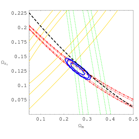
The parametrization (137) of the Hubble parameter together with the normalization (138) can be used to place observational constraints on the DGP model at the background level DGPobser1 ; DGPobser2 ; DGPobser3 ; DGPobser4 ; DGPobser5 . In Ref. DGPobser1 the authors found a significantly worse fit to Supernova Ia (SN Ia) data and the distance to the last-scattering surface WMAP1 relative to the CDM model. In Refs. DGPobser2 and DGPobser4 the authors showed that the flat DGP model is disfavored from the combined data analysis of SN Ia Riess04 ; Astier05 and BAO BAO1 . In Fig. 3 we show the joint observational constraints DGPobser3 from the data of SNLS Astier05 , BAO BAO1 , and the CMB shift parameter WMAP3 . While the flat DGP model can be consistent with the SN Ia data, it is under strong observational pressure by adding the data of BAO and the CMB shift parameter. The open DGP model gives a slightly better fit relative to the flat model DGPobser3 ; DGPobser5 . The joint analysis using the data of SN Ia, BAO, CMB, gamma ray bursts, and the linear growth factor of matter perturbations show that the flat DGP model is incompatible with current observations DGPobser6 .
In the DGP model a brane-bending mode (i.e. longitudinal graviton) gives rise to a field self-interaction of the form through a mixing with the transverse graviton DGPnon1 ; DGPnon2 . This can lead to the decoupling of the field from gravitational dynamics in the local region by the so-called Vainshtein mechanism Vainshtein . The General Relativistic behavior can be recovered within a radius , where is the Schwarzschild radius of a source. Since is larger than the solar-system scales, the DGP model can evade local gravity constraints DGPnon1 ; Gruzinov:2001hp ; DGPnon2 . However the DGP model is plagued by a strong coupling problem for typical distances smaller than 1000 km Luty . Some regularization methods have been proposed to avoid the strong coupling problem, such as smoothing out the delta profile on the brane Kolano1 ; Kolano2 or re-using the delta function profile but in a higher-dimensional brane CascoDGP ; CascoDGP2 ; CascoDGP3 .
As we will see in VII.3, the analysis of 5D cosmological perturbations on the scales larger than shows that the DGP model contains a ghost mode in the scalar sector of the gravitational field DGPghost1 ; DGPghost2 ; DGPghost3 . There are several ways of the generalization of the DGP model to avoid the appearance of ghosts. One way is to consider the 6D braneworld set-up as in the Cascading gravity deRham . Another is to generalize the field self-interaction term to more general forms in the 4D gravity Nicolis . In Sec. V we shall discuss the latter approach (“Galileon gravity”) in detail.
V Galileon gravity
In the DGP model the field derivative self-coupling , arising from a brane-bending mode, allows the decoupling of the field from matter within a Vainshtein radius. In the local regions where solar-system experiments are carried out, the field is nearly frozen through the non-linear self-interaction. This is different from the chameleon mechanism in which the presence of the field potential with a matter coupling gives rise to a minimum with a large mass in the regions of high density.
Under the Galilean shift , the field equation following from the Lagrangian is unchanged in the Minkowski space-time. The generalization of the nonlinear field Lagrangian to more general cases may be useful, e.g., to overcome the ghost problem associated with the DGP model. In fact Nicolis et al. Nicolis derived five Lagrangians that lead to the field equations invariant under the Galilean shift in the Minkowski space-time. The scalar field respecting the Galilean symmetry is dubbed “Galileon”. Each of the five terms only leads to second-order differential equations, keeping the theory free from unstable spin-2 ghost degrees of freedom.
If we extend the analysis in Ref. Nicolis to that in the curved space-time, the Lagrangians should be promoted to covariant forms. Deffayet et al. Deffayetga1 ; Deffayetga2 derived covariant Lagrangians () that keep the field equations up to second-order, while recovering the five Lagrangians derived by Nicolis et al. in the Minkowski space-time. This can be achieved by introducing field-derivative couplings with the Ricci scalar and the Einstein tensor in the expression of . Since the existence of those terms affects the effective gravitational coupling, the Galileon gravity based on the covariant Lagrangians () can be classified as one of modified gravitational theories.
The cosmological dynamics including the terms up to and have been studied by a number of authors Sami10 ; DT2 . In particular Refs. DT2 ; DT3 have shown that, for the covariant Galileon theory having de Sitter attractors, cosmological solutions with different initial conditions converge to a common trajectory– a tracker solution. Moreover there is a viable parameter space in which the conditions for the avoidance of ghosts and Laplacian instabilities of scalar and tensor perturbations are satisfied.
The generalization of Galileon gravity, which mostly corresponds to the modification of the term , has been also extensively studied recently JustinGal -Hirano . One application is to introduce the non-linear field self-interaction of the form in the action of (generalized) Brans-Dicke theories KazuyaGal ; Kobayashi1 ; Kobayashi2 ; DT1 ; DMT , where is a function of . For suitable choices of the function , there exist de Sitter (dS) solutions responsible for dark energy even in the absence of the field potential. The cosmology based on a further general term has been discussed in the context of either dark energy and inflation KYY ; DPSV ; Mizuno ; Burrage ; Kimura ; Kamada ; Hirano .
In the following we review the cosmological dynamics in the Galileon dark energy model based on the covariant Lagrangians () and study observational constraints on the model. We will also discuss the modified version of Galileon gravity in which the term is generalized.
V.1 Cosmology of a covariant Galileon field
We start with the covariant Galileon gravity described by the action Deffayetga1 ; Deffayetga2
| (140) |
where is the reduced Planck mass, and ’s are constants. The five Lagrangians () satisfying the Galilean symmetry in the limit of the Minkowski space-time are given by
| (141) |
where is a constant having a dimension of mass, and is the Einstein tensor. For the matter Lagrangian we take into account perfect fluids of non-relativistic matter (energy density , equation of state ) and radiation (energy density , equation of state ).
Let us consider the FLRW metric with the cosmic curvature :
| (142) |
Variation of the action (140) with respect to leads to the following equations of motion
| (143) | |||
| (144) |
where , and
| (145) | |||||
| (146) | |||||
The matter fluids satisfy the continuity equations and . We define the dark energy equation of state and the effective equation of state , as
| (147) |
Using the continuity equation , it follows that .
Since we are interested in the case where the late-time cosmic acceleration is realized by the field kinetic energy, we set in the following discussion555In this case the only solution in the Minkowski background () corresponds to for .. Then the de Sitter solution () can be present for . We normalize the mass to be , which gives for . Defining , Eqs. (143) and (144) lead to the following relations at the de Sitter solution:
| (148) |
where
| (149) |
It is convenient to use the variables and , because the coefficients of physical quantities and dynamical equations can be expressed by and . The relations (148) do not change under the rescaling and , where is a real constant. Then the rescaled choice of can provide the same physics.
In order to study the cosmological dynamics, we introduce the following dimensionless variables:
| (150) |
At the de Sitter solution and . We define the dark energy density parameter
| (151) |
Then Eq. (143) can be written as , where , , and .
The autonomous equations for the variables , , , and are given by DT3 ; Nesseris10 :
| (152) | |||||
| (153) | |||||
| (154) | |||||
| (155) |
where a prime represents a derivative with respect to , and
| (156) | |||||
The Hubble parameter follows from the equation . The solutions to Eqs. (154) and (155) are given by and respectively, where the subscript “(0)” represents the values today ().
From Eqs. (152) and (153) we find that there are three distinct fixed points: (A) , (B) , and (C) . As we have already mentioned, the point (C) corresponds to the de Sitter solution. By considering homogeneous perturbations about this point, we can show that the de Sitter solution (C) is always classically stable DT3 . The point (B) is a tracker solution found in Ref. DT2 , along which the field velocity evolves as . During the radiation and matter eras the variable is much smaller than 1. The fixed point (B) is followed by the stable de Sitter point (C) once grows to the order of 1. If the initial conditions of both and in the radiation era are much smaller than 1, then the solutions are close to the point (A) at the initial stage. At late times the solutions approach the tracker at . Depending on the initial values of , the epoch at which the solutions reach the tracker is different. In the following we consider the background evolution in two regimes: (i) and (ii) in more detail.
V.1.1 Tracker solution
Along the tracker () the dark energy density parameter (151) is given by
| (157) |
which is much smaller than 1 during the radiation and matter eras. From Eqs. (154) and (155) we obtain . This is integrated to give
| (158) |
where is a constant. From Eqs. (153) and (154) we have , which is integrated to give
| (159) |
Substituting Eqs. (158) and (159) into Eq. (154), we obtain the cosmologically viable solution to , as
| (160) |
where is another constant. Since the density parameter (160) evolves as in the early time (), this demands the condition (provided ). Using the density parameters today, the constants and can be expressed as and . Since , we have . Using Eq. (160), the Hubble parameter can be expressed in terms of the redshift :
| (161) | |||||
which is useful to test the viability of the tracker solution from observations.
On the tracker, the equations of state defined in Eq. (147) are given by
| (162) |
During the cosmological sequence of radiation (, , ), matter (, , ), and de Sitter (, , ) eras, the dark energy equation of state evolves as , whereas the effective equation of state evolves as . This peculiar evolution of for the tracker corresponds to the case (e) in Fig. 4. Although the effect of the cosmic curvature does not affect the dynamics of significantly, it can change the diameter distance as well as the luminosity distance relative to the flat Universe.
The epoch at which the solutions reach the tracking regime depends on model parameters and initial conditions. The approach to this regime occurs later for smaller initial values of , see Fig. 4. In Ref. DT3 it was shown that the tracker is stable in the direction of by considering a homogeneous perturbation . This means that once the solutions reach the tracker the variable does not repel away from 1. If initially, numerical simulations show that the solutions approach the tracker with the late-time cosmic acceleration. Meanwhile, for the initial conditions with , the dominant contribution to comes from the Lagrangian , so that the field energy density decreases rapidly as in the standard massless scalar field.

V.1.2 Solutions in the regime
There is another case in which the solutions start to evolve from the regime (where the term gives the dominant contribution to the field dynamics). In this regime, the variables and satisfy the following approximate equations
| (163) |
As long as , the evolution of and during the radiation (matter) era is given by and ( and ). Then the field velocity grows as during the radiation era and during the matter era. The evolution of is slower than that for the tracker (i.e. ).
In the regime the equations of state are
| (164) |
Provided that , one has during the radiation era and during the matter era. This evolution of is quite different from that for the tracker solution.
In Fig. 4 the variation of is plotted for a number of different initial conditions with [which correspond to the cases (a)-(d)]. As expected, the solutions start to evolve from the value in the radiation era. For larger initial values of they approach the tracker earlier. This tracking behavior also occurs in the presence of the cosmic curvature Nesseris10 .
V.1.3 Conditions for the avoidance of ghosts and Laplacian instabilities
Let us find a model parameter space in which the appearance of ghosts and instabilities can be avoided in covariant Galileon gravity. In doing so, we need to study a linear perturbation theory on the FLRW background. For simplicity we focus on the flat Universe with . Let us consider the perturbed metric
| (165) |
where , , and are scalar metric perturbations. We have chosen the gauge without a non-diagonal scalar perturbation in the spatial part of the metric, i.e. Bardeen . Taking into account two perfect fluids with the equations of state (), there are three propagating scalar degrees of freedom. The velocity potentials () of perfect fluids are related with the energy-momentum tensor , as ().
Introducing the vector and expanding the action (140) up to the second-order, we obtain the second-order action for scalar perturbations DT3 (see also Refs. Faddeev ; Suyama ; DMT ):
| (166) |
where the fields and are integrated out. , and are symmetric matrices and is an antisymmetric matrix (for which we do not write explicit forms).
In order to avoid the appearance of ghosts we require that the matrix is positive definite. This corresponds to the conditions , , and
| (167) |
where
| (168) | |||
| (169) | |||
| (170) |
The propagation speeds of three scalar degrees of freedom are known by solving the equation
| (171) |
For the two perfect fluids we have and , which are are positive for both radiation and non-relativistic matter. The third stability condition associated with another scalar degree of freedom is given by
| (172) |
where
| (173) |
Let us consider tensor perturbations with , where is traceless () and divergence-free (). We expand the action (140) at second-order in terms of the two polarization modes, , where and are the polarization tensors. For the polarization mode , the second-order action is given by
| (174) |
The conditions for the avoidance of ghosts and Laplacian instabilities of tensor perturbations correspond, respectively, to
| (175) | |||
| (176) |
The same conditions also follow from .
In the regime and one has and . For the initial conditions with we require that to avoid the scalar ghost. Since and , there are no Laplacian instabilities of scalar and tensor perturbations in this regime.
In the tracking regime characterized by (either or ), the conditions (167), (172), (175), and (176) give the bounds on the parameters and . In the regime these conditions translate to
| (177) | |||
| (178) |
For the branch the first condition reduces to . Since and , the tensor modes do not provide additional constraints. At the de Sitter point () we require that
| (179) | |||
| (180) |
If , it can happen that has a minimum during the transition from the regime to DT2 ; DT3 . This value tends to decrease as approaches 1. Imposing that at the minimum, we obtain the bound
| (181) |
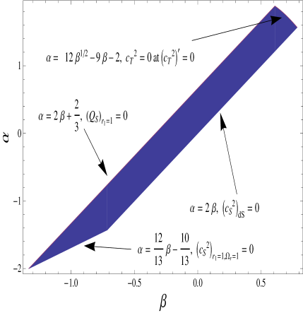
In Fig. 5 we plot the parameter space in the plane constrained by the conditions (177)-(181). Clearly there are viable model parameters satisfying all the theoretical constraints.
V.1.4 Observational constraints on Galileon cosmology from the background cosmic expansion history
Since the evolution of the dark energy equation of state in covariant Galileon gravity is rather peculiar, the observational data related with the background cosmic expansion history may place tight constraints on the model. Especially the analytic formula (161) for the tracker is useful for such a purpose. In Ref. Nesseris10 the authors confronted the Galileon model by using the observational data of SN Ia (Constitution Hicken and Union2 sets Amanullah ), the CMB (WMAP7) shift parameters WMAP7 , and BAO (SDSS7) BAO2 .
If either of the SN Ia data (Constitution or Union2) is used in the data analysis, the for the tracker is similar to that in the CDM model. In the presence of the cosmic curvature , the tracker solution is compatible with the individual observational bound constrained from either CMB or BAO. However, the combined data analysis of Constitution+BAO+CMB shows that the difference of between the tracker and the CDM is (or ). This means that the tracker is severely disfavored with respect to the CDM. A similar conclusion was reached from the combined data analysis of Union2+BAO+CMB. The reason for this incompatibility is that the SN Ia data favor the large values of (), whereas the CMB and BAO data constrain smaller values of .
The general solutions starting from the regime finally approach the tracker as grows to 1. In Ref. Nesseris10 the authors carried out the likelihood analysis for such general solutions and found that the solutions approaching the tracker at late times (such as the case (a) in Fig. 4) are favored from the combined data analysis. In the flat FLRW background the best-fit model parameters are , (ConstitutionCMBBAO, 68 % CL), and , (Union2CMBBAO, 68 % CL).
For several fixed values of it was shown that the late-time tracking solutions can be consistent with the data, apart from the models with largely negative such as . For example, the general solutions with and the model parameters give the similar value of to that in the the CDM. In this case the Akaike-Information-Criteiron (AIC) statistics AIC also have the same support for the two models (see also Ref. Liddle04 )
The Bayesian-Information-Criterion (BIC) statistics BIC show that the general solutions, with all 4 parameters are varied, are not particularly favored over the CDM model. This mainly comes from the statistical property that the numbers of model parameters are larger than those in the flat CDM. In fact the late-time tracking solutions with a non-zero cosmic curvature can be well consistent with the combined data analysis at the background level.
V.2 Generalized Galileon gravity
In Sec. III we showed that in Brans-Dicke theory with the coupling of the order of unity the presence of the field potential allows a possibility for the consistency with local gravity constraints through the chameleon mechanism. Another way to recover the General Relativistic behavior in the regions of high density is to introduce the Galileon-like field self-interaction. Silva and Koyama KazuyaGal studied Brans-Dicke theory in the presence of the term [which is the generalization of the term ]. The action of this theory is given by
| (182) |
If , there exists a de Sitter solution that can be responsible for the late-time acceleration. As in the Galileon model discussed in Sec. V.1 the field is nearly frozen during the radiation and matter eras through the cosmological Vainshtein mechanism, but it finally approaches the de Sitter solution characterized by constant. Moreover, as in the DGP model, the Vainshtein radius can be much larger than the solar system scale, so that the General Relativistic behavior can be recovered in the local region KazuyaGal .
We may consider more general theories described by the action DT1
| (183) |
where , and , , are functions of . From the requirement of having de Sitter solutions responsible for dark energy, it is possible to restrict the functional forms of , , and . In the presence of non-relativistic matter (energy density ) and radiation (energy density ), the field equations are given by
| (184) | |||
| (185) |
where . Let us search for de Sitter solutions at which and are constants. If and are power-law functions of , the quantities such as , , and remain constants. Provided that and , we can solve Eqs. (184) and (185) for and at the de Sitter point. These conditions are satisfied for the following functions
| (186) |
where GeV is the reduced Planck mass, is a constant having a dimension of mass, and and are dimensionless constants. One can show that the coupling must be positive for the consistency of theories DT1 . The Brans-Dicke theory described by the action (182) corresponds to with the Brans-Dicke parameter . Since is constant for , the theory with corresponds to k-essence minimally coupled gravity.
From Eqs. (184) and (185) we obtain the following algebraic equations at the de Sitter fixed point:
| (187) | |||||
| (188) |
where and are the values of and at the de Sitter point, respectively. We fix the mass scale to be , where we have used . For given and , the quantity is determined by solving Eq. (187). Then the dimensionless constant is known from Eq. (188).
In order to recover the General Relativistic behavior in the early cosmological epoch we require that the field initial value is close to from Eq. (186). The quantity is much smaller than 1 in the early cosmological epoch, so that the field is nearly frozen during the radiation and matter eras. The field starts to evolve at the late cosmological epoch in which grows to the order of unity. Introducing the dimensionless quantities and , one can show that the fixed point corresponding to the matter era corresponds to DT1 . Since is positive definite, it follows that .
The conditions for the avoidance of ghosts and Laplacian instabilities are known by employing the method presented in Sec. V.1.3. Provided , we require that to avoid ghosts during the cosmological evolution from the radiation era to the epoch of cosmic acceleration DT1 . The stability of the de Sitter point is automatically ensured for and . From Eq. (187) the parameter is restricted in the range
| (189) |
The field propagation speed squared during the radiation and matter eras is given by and , respectively in which case no instabilities of linear perturbations are present. Meanwhile, at the de Sitter solution, we have DT1
| (190) |
which is positive for . Hence the parameter is restricted in the range
| (191) |
which includes Brans-Dicke theory with the action (182) as a specific case ().
In Ref. Kobayashi1 the authors studied the evolution of matter density perturbations and showed that, for the model with , there is an anti-correlation between the cross-correlation of large scale structure and the integrated Sachs-Wolfe effect in CMB anisotropies. We shall discuss the main reason of this anti-correlation in Sec. VII.4. This property will be useful to distinguish the above model from the CDM in future observations.
VI Other modified gravity models of dark energy
In this section we briefly discuss other classes of modified gravity models of dark energy. These include (i) Gauss-Bonnet gravity with a scalar coupling , (ii) gravity, and (iii) Lorentz-violating models.
VI.1 Gauss-Bonnet gravity with a scalar coupling
In addition to the Ricci scalar , we can construct other scalar quantities coming from the Ricci tensor and the Riemann tensor , i.e. and Kret . It is possible to avoid the appearance of spurious spin-2 ghosts by taking a Gauss-Bonnet (GB) combination Stelle ; Barth ; ANunez , defined by
| (192) |
A simple model that can be responsible for the cosmic acceleration today is NOS05
| (193) |
where and are functions of a scalar field . The coupling of the field with the GB term appears in low-energy effective string theory Gasreview . For the exponential potential and the coupling , the cosmological dynamics were studied in Refs. NOS05 ; Koivisto1 ; TsujiSami07 ; Koivisto2 ; Neupane06 ; Neupane ; Sanyal . In this model there exists a de Sitter solution due to the presence of the GB term. In Refs. Koivisto1 ; TsujiSami07 it was also found that the late-time de-Sitter solution is preceded by a scaling matter era.
Koivisto and Mota Koivisto1 placed observational constraints on the model (193) with the exponential potential , by using the Gold data set of SN Ia together with the CMB shift parameter data of WMAP. The parameter is constrained to be at the 95% confidence level. In Ref. Koivisto2 , they also included the constraints coming from the BAO, LSS, big bang nucleosynthesis, and solar system data. This joint analysis showed that the model is strongly disfavored by the data. In Ref. TsujiSami07 it was also found that tensor perturbations are subject to negative instabilities when the GB term dominates the dynamics (see also Refs. Kawai ; Ohta for related works).
Amendola et al. AmenDavis studied local gravity constraints on the above model and showed that the density parameter coming from the GB term is required to be strongly suppressed for the compatibility with solar-system experiments (which is typically of the order of ). The above discussion indicates that the GB term with the scalar-field coupling can hardly be the source for dark energy.
VI.2 gravity
The general Lagrangian including the scalar quantities constructed from the Ricci scalar , the Ricci tensor and the Riemann tensor is given by . The dark energy models based on these theories have been studied in Refs. CaDe ; Calcagni05 ; Sami05 ; Chibaghost ; Mena ; Hervik ; Cognola ; Sokolowski . In order to avoid spurious spin-2 ghosts we need to choose the GB combination (192), i.e. Defelice1 ; Defelice2 .
The cosmological dynamics based on the action,
| (194) |
have been studied by a number of authors NO05 ; Cognola06 ; LBM ; DeTsu ; Cope09 ; Mohseni ; Ishak . In order to ensure the stability of radiation/matter solutions, we need to satisfy the condition for all . We also require the regularities of the functions , , and DeTsu . There exists a de Sitter solution responsible for dark energy, whose stability requires the condition . Moreover must approach in the limit .
In Ref. DeTsu the authors proposed a number of models satisfying these conditions (see also Ref. Cope09 ). One of such models is given by
| (195) |
where , and are constants. The numerical simulation of Ref. DeTsu shows that the model (195) is cosmologically viable at least at the background level. Moreover it can be consistent with solar-system constraints for a wide range of model parameters DeFelicesolar .
In order to study the viability of the theories described by the action (194) further, let us consider the evolution of matter density perturbations in the presence of a perfect fluid with the barotropic equation of state . In Ref. DMT10 it was shown that, for small scales (i.e. for large momenta ), there are two different scalar propagation speeds. One of them corresponds to the mode for the fluid, i.e. , whereas another is given by
| (196) |
where
| (197) |
The parameter characterizes the deviation from the CDM model (note that the linear term does not give rise to any contribution to the field equation). For viable models we have at high redshifts DeTsu . Since the background evolution during the radiation/matter domination is given by and , it follows that
| (198) |
The Laplacian instability at small scales is absent only for . Since and during the radiation and matter eras, respectively, the perturbations with large momentum modes are unstable. This leads to violent growth of matter density perturbations incompatible with the observations of large-scale structure LBM ; DMT10 .
By considering the full perturbation equations, one can show that the onset of the negative instability corresponds to DMT10
| (199) |
Even when is much smaller than 1, we can always find a wave number satisfying the condition (199). For the scales smaller than that determined by the wave number in Eq. (199), the linear perturbation theory breaks down. Hence the background solutions cannot be trusted for those scales, which makes the theory unpredictable. The Laplacian instability can be avoided only for , which corresponds to the CDM model. The above property persists irrespective of the forms of .
For more general theories described by the Lagrangian density it is possible to avoid such Laplacian instabilities Gerrard , depending on the models Suyama10 (see also Refs. Alimo08 ; Alimo09 ; Elizalde10 ; Tanaka ). It may be of interest to construct some viable dark energy models in such theories.
VI.3 Lorentz violating models
The modified gravity models such as gravity and Galileon gravity can give rise to the phantom dark energy equation of state without violating the conditions for the appearance of ghosts and instabilities. In the models with a broken Lorentz invariance it is also possible to realize without pathological behavior in the Ultra-Violet (UV) region gcondensate ; Rubakov ; Libanov (see also Ref. Rubakovreview for a review). In order to construct Lorentz violating models without pathological behavior of phantoms, one may start with a field theory consistent at energy scales from zero to the UV cutoff scale and then deform the theory in the Infra-Red (IR) in such a way that its behavior at high energies remains healthy. Although the weak energy condition is violated in the homogenous background, pathological states are present below a certain low scale only. Provided that is close to the Hubble scale, a theory of this sort should be acceptable.
Let us consider a Lorentz violating model with two-derivative kinetic terms with healthy behavior below the scale Ben plus one-derivative term suppressed by the small parameter MLVR . The model has a vector field and a scalar field with a potential . The Lagrangian is given by Rubakov ; Libanov
| (200) | |||
| (201) | |||
| (202) |
where ( is the UV cut-off scale). The dimensionless parameters and are the functions of , and is a free positive parameter that characterizes an IR scale. The Lorentz invariance is broken for .
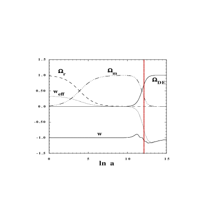
In spatially homogeneous background we have
| (203) |
where and are time and space components of . In the flat FLRW background with non-relativistic matter and radiation for the matter Lagrangian , we obtain the following equations of motion
| (204) | |||
| (205) | |||
| (206) |
where .
For the separable potential with constant the cosmological dynamics of the above system have been studied in detail in Refs. Rubakov ; Libanov . In what follows we assume that both and are constants. Provided one can show that there is a de Sitter solution with , at which and are frozen. In the early cosmological epoch the field is close to 0, whereas the field slowly rolls down its potential (with the energy density dominating over that of ).
Prior to the epoch of de Sitter cosmic acceleration there is a transient phantom regime () characterized by in which the field rolls up its potential. The Hubble parameter slowly increases toward the de Sitter value . In Fig. 6 we plot the evolution of the dark energy equation of state and the effective equation of state together with the density parameters of dark energy, non-relativistic matter, and radiation666Here the definition of and is and .. Clearly the solution undergoes the period with before reaching the de Sitter attractor.
The phantom equation of state can be realized without having ghosts, tachyons or superluminal modes in the UV region. In the IR region characterized by , either tachyons or ghosts appear for the spatial momenta smaller than Rubakov ; Libanov . The presence of tachyons at IR scales leads to the amplification of large-scale field perturbations whose wavelengths are roughly comparable to the present Hubble radius. There are two tachyonic regions of spatial momenta in this model: (a) one is sub-horizon and its momenta are characterized by ; (b) another is super-horizon with the momenta . In the region (a) there is a parameter space in which the perturbations always remain smaller than the homogenous fields. In the region (b) the growth of the perturbations is suppressed by the factor .
There are other classes of Lorentz violating models such as ghost condensate gcondensate and Horava-Lifshitz gravity Horava (see also Refs. LVmodels1 -LVmodelsf ). The application of such scenarios to dark energy has been studied by a number of authors, see e.g., Piazza ; Sari ; Park . It remains to to see whether such Lorentz-violating models can be observationally distinguished from other dark energy models.
VII Observational signatures of modified gravity
In order to confront modified gravity models with the observations of large-scale structure and CMB, we discuss the evolution of density perturbations in four modified gravity models: (i) gravity, (ii) scalar-tensor gravity, (iii) DGP braneworld model, and (iv) Galileon gravity. We also discuss observables to confront with weak lensing observations.
VII.1 gravity
Let us first consider metric gravity in the presence of non-relativistic matter. We take the following perturbed metric in a longitudinal gauge about the flat FLRW background with scalar metric perturbations and Bardeen
| (207) |
The energy momentum tensors of a non-relativistic perfect fluid are decomposed into background and perturbed parts, as and ( is a velocity potential).
The equations for matter perturbations, in the Fourier space, are given by Kodama ; Robert ; Bassett
| (208) | |||
| (209) |
where is a comoving wave number. We define the gauge-invariant matter density perturbation , as
| (210) |
Then Eqs. (208) and (209) yield
| (211) | |||
| (212) |
from which we obtain
| (213) |
where .
In gravity the quantity has a perturbation . In the following we use the unit , but we restore gravitational constant when it is required. For the action given in Eq. (2), we obtain the linearized perturbation equations in Fourier space Kofman87 ; Hwang02 ; Hwang
| (214) | |||
| (215) | |||
| (216) |
In Eq. (215) we have introduced the mass term
| (217) |
For viable dark energy models the condition is satisfied during most of the cosmological epoch, so that Star07 ; Tsuji08 . This is equivalent to the mass squared introduced in Eq. (43), which is required to be positive to avoid the tachyonic instability.
For the observations of large-scale structure and weak lensing we are interested in the modes deep inside the Hubble radius (). In the following we employ the quasi-static approximation under which the dominant terms in Eqs. (213)-(216) correspond to those including , (or ) and Star98 ; Boi00 ; review5 ; Tsujimatterper ; TsujiUddin ; Hwang10 . We then obtain the following approximate relations from Eqs. (213)-(216) :
| (218) | |||
| (219) | |||
| (220) |
The evolution of perturbations is different depending on whether is larger or smaller than . We shall discuss two cases: (A) and (B) , separately. For viable models the mass squared is large in the past and it gradually decreases with time. Hence the transition from the regime (A) to the regime (B) can occur in the past, depending on the wave numbers .
VII.1.1 Evolution of perturbations in the regime:
The solutions to Eq. (220) are given by the sum of the oscillating solution obtained by setting and the special solution of Eq. (220) induced by the presence of matter perturbations . The oscillating part satisfies the equation . Using the WKB approximation, we obtain the following solution Star07
| (221) |
where we have used the approximation .
For the analytic estimation of the oscillating mode we take the model (47), which corresponds to the asymptotic form of the models (45) and (46) in the region . During the matter era in which the background Ricci scalar evolves as , the quantity has a dependence for the model (47). Then the evolution of the perturbation, , is given by
| (222) |
where and are constants. Unless the coefficient is chosen to be very small, as we go back to the past, the perturbation dominates over the background value . Since the Ricci scalar can be negative, this leads to the violation of the stability conditions ( and ).
The special solution to Eq. (220) can be derived by neglecting the first and second terms relative to others, giving
| (223) |
Under the condition , one has and hence . Then the matter perturbation equation (218) reduces to
| (224) |
where we have reproduced the gravitational constant . In Refs. delaCruz08 ; Motohashi the perturbation equations have been derived without neglecting the oscillating mode.
During the matter-dominated epoch (), Eq. (224) has the growing-mode solution
| (225) |
This is the same evolution as that in standard General Relativity. From Eq. (223) the matter-induced mode evolves as and . Compared to the oscillating mode (222), decreases more slowly and hence it dominates over at late times. The evolution of the perturbation relative to the background value is given by
| (226) |
where and are constants. In order to avoid the dominance of the oscillating mode at the early cosmological epoch, we require that the coefficient is suppressed relative to Star07 ; Tsuji08 ; Appleos1 .
This fine-tuning of initial conditions is related with the singularity problem raised by Frolov Frolov . The field in the Einstein frame has a weak singularity at (at which the curvature and the mass go to infinity with a finite potential ). Unless the oscillating mode of the field perturbation is strongly suppressed relative to the background field , the system can access the curvature singularity. This past singularity can be cured by taking into account the term Appleos2 . Note that the models proposed in Ref. Miranda [e.g., ] to cure the singularity problem satisfy neither the local gravity constraints Thongkool nor observational constraints of large-scale structure delaCruz . There are some works for the construction of unified models of inflation and dark energy based on theories fRearly4 ; NOuni1 ; NOuni2 , but the smooth transition between two accelerated epochs without crossing the point is not easy unless the forms of are carefully chosen Appleos2 .
VII.1.2 Evolution of perturbations in the regime:
Since the mass decreases as , the modes initially in the region can enter the regime during the matter-dominated epoch. It is sufficient to consider the matter-induced mode because the oscillating mode is already suppressed during the evolution in the regime . The matter-induced special solution of Eq. (220) in the regime is approximately given by
| (227) |
From Eq. (219) the gravitational potentials satisfy
| (228) |
Plugging Eq. (228) into Eq. (218), the matter perturbation obeys the following equation
| (229) |
During the matter-dominated epoch ( and ), we obtain the following evolution
| (230) |
The growth rate of gets larger compared to that in the regime .
VII.1.3 Matter power spectra and the ISW effect
If the transition from the regime to the regime occurs during the matter era, the evolution of matter perturbations changes from to . We use the subscript “” for the quantities at which is equal to , whereas the subscript “” is used at which the accelerated expansion starts (). While the redshift is independent of , depend on and also on the mass .
For the model (47) the variable can grow fast from the regime (i.e., to the regime (i.e., . In fact, can grow to the order of even if is much smaller than in the deep matter era. For the sub-horizon modes relevant to the galaxy power spectrum, the transition at typically occurs at the redshift larger than 1 (provided that ). For the mode one has for and for . As gets larger, the period of non-standard evolution of becomes shorter because tends to be smaller. Since the scalaron mass evolves as for the model (47), the time has a scale-dependence . This means that the smaller-scale modes cross the transition point earlier. The matter power spectrum at the time shows a difference compared to the case of the CDM model:
| (231) |
From Fig. 7 we find that the matter power spectrum in the model (47) with is in fact larger than that in the CDM model on smaller scales.

The galaxy matter power spectrum is modified by this effect. Meanwhile the CMB spectrum is hardly affected except for very large scales (for the multipoles ) at which the Integrated Sachs-Wolfe (ISW) effect becomes important. Hence there is a difference for the spectral indices of two power spectra, i.e.
| (232) |
For larger the redshift can be as close as , which means that the estimation (232) is not necessarily valid in such cases. Moreover the estimation (232) does not take into account the evolution of after to the present epoch (). It was found in Ref. Tsuji08 that the estimation (232) agrees well with the numerically obtained for .
In order to discuss the growth rate of matter perturbations, it is customary to introduce the growth index Peebles
| (233) |
where . In the CDM model is nearly constant for the redshifts , i.e. Wang98 ; Linder05 . In gravity, if the perturbations are in the GR regime () today, is close to 0.55. On the other hand, if the transition to the scalar-tensor regime occurs at the redshift larger than 1, the growth index tends to be smaller than 0.55 Moraes08 ; Moraes09 . Since , the smaller implies a larger growth rate.
For the wave numbers relevant to the linear regime of the matter power spectra (, where ) the viable models (45)-(48) can give rise to the growth index today. Depending on the wave numbers , can be dispersed in the regime , or can show the convergence in the regime Moraes08 ; Moraes09 . Moreover, when is small, the growth index exhibits a large variation even for low redshifts (). Although the present observational constraints on are quite weak, the unusual evolution of can be useful to distinguish the models from the CDM in future observations.
After the system enters the epoch of cosmic acceleration, the wave number can again become smaller than . Hence the -dependence is not necessarily negligible even for . However numerical simulations show that is not much different from derived by Eq. (232) Tsuji08 . Thus the analytic estimation (232) is certainly reliable to place constraints on model parameters except for . Observationally we do not find any strong difference for the slopes of the spectra of LSS and CMB. If we take the mild bound , we obtain the constraint Star07 . In this case the local gravity constraint (67) is also satisfied.
For the wave numbers we need to take into account the non-linear effect of density perturbations. In Refs. Oyaizu1 ; Oyaizu2 ; Oyaizu3 ; ZhaoLi the authors carried out -body simulations for the model (46) (see also Refs. Stabenau ; Laszlo ). Hu and Sawicki (HS) Huparametrization proposed a fitting formula to describe the non-linear power spectrum based on the halo model. Koyama et al. Koyama09 studied the validity of the HS fitting formula by comparing it with the results of -body simulations and showed that the HS fitting formula can reproduce the power spectrum in -body simulations for the scales Mpc-1. In the quasi non-linear regime a normalized skewness, , has been evaluated in gravity and in Brans-Dicke theories Tateskew . The skewness in dark energy models differs only by a few percent relative to the value in the CDM model.
The modified growth of matter perturbations also affects the evolution of the gravitational potentials and . The effective potential is important to discuss the ISW effect on the CMB as well as the weak lensing observations Kunz . For the modes deep inside the Hubble radius, Eq. (219) gives
| (234) |
Note that for the large-scale modes relevant to the ISW effect in CMB we need to solve the full perturbation equations without using the quasi-static approximation on sub-horizon scales. For viable models, however, numerical simulations show that the result (234) can be trustable even for the wave numbers close to the Hubble radius today (i.e. ) TsujiUddin . In the CDM model the potential remains constant during the standard matter era, but it decays after the system enters the accelerated epoch, producing the ISW contribution for low multipoles on the CMB power spectrum. In gravity the additional growth of matter perturbations in the region changes the evolution of .
From the observation of the CMB angular power spectrum, the constraint on the deviation parameter from the CDM is weak. The value of today is constrained to be Peiris . There is another observational constraint coming from the angular correlation between the CMB temperature field and the galaxy number density field induced by the ISW effect. The avoidance of a large anti-correlation between the observational data of CMB and LSS places an upper bound of . Since this roughy corresponds to , the CMB observations do not provide tight constraints on models relative to the matter power spectrum of LSS. In weak lensing observations, the modified evolution of the lensing potential directly leads to the change even for the small-scale shear power spectrum Kunz ; TsujiTate ; Schmidt . Hence this can be a powerful tool to constrain gravity models from future observations.
VII.2 Brans-Dicke theory
Let us proceed to discuss the evolution of matter perturbations in Bran-Dicke theory described by the action (76) with the potential and the coupling . We are mainly interested in large coupling models with of the order of unity KW1 ; KW2 ; TUMTY , as this gives rise to significant deviation from the CDM. We define the field mass squared to be . If the scalar field is light such that the condition is always satisfied irrespective of high or low density regions, the coupling is constrained to be from local gravity constraints. Meanwhile, if the mass in the region of high density is much larger than that on cosmological scales, the model can satisfy local gravity constraints under the chameleon mechanism even if is of the order of unity. Cosmologically the mass can decrease from the past to the present, which can allow the transition from the “GR regime” to the “scalar-tensor regime” as it happens in gravity. An example of the field potential showing this behavior is given by Eq. (98).
As in gravity, the matter perturbation obeys Eq. (213). The difference appears in the expression of the gravitational potential . In Fourier space the scalar metric perturbations obey the following equations Hwang02 ; Hwang ; TUMTY
| (235) | |||
| (236) | |||
| (237) |
where is the perturbation of the field , , and
| (238) |
Provided that the field is sufficiently heavy to satisfy the conditions , one can employ the approximation in Eq. (236). The solution to Eq. (236) consists of the sum of the matter-induced mode sourced by the matter perturbation and the oscillating mode , i.e. (as in the case of gravity).
In order to know the evolution of the matter-induced mode we employ the quasi-static approximation on sub-horizon scales. Under this approximation, we have from Eqs. (235) and (238), where the subscript “ind” represents the matter-induced mode. Then from Eq. (236) we find
| (239) |
Using Eqs. (235) and (237) we obtain
| (240) |
In the massive limit , we recover the standard result of General Relativity. In the massless limit , it follows that and .
Plugging Eq. (240) into Eq. (218), we obtain the equation for matter perturbations TUMTY
| (241) |
where the effective gravitational coupling is
| (242) |
We have recovered the bare gravitational constant . In the massless limit () this reduces to
| (243) |
where in the last line we have used the relation (77) between the coupling and the Brans-Dicke parameter . In gravity we have and hence .
Let us consider the evolution of the oscillating mode of perturbations. Using Eqs. (235) and (236) for sub-horizon modes (), the gravitational potentials can be expressed by (note that for the oscillating mode). From Eq. (238) the perturbation of corresponding to the oscillating mode is given by
| (244) |
Substituting Eq. (244) into Eq. (236), it follows that
| (245) |
which is valid in the regime .
When the field potential is required to be heavy in the region of high density for the consistency with local gravity constraints. We take the potential (98) as an example of a viable model. During the matter era the field settles down at the instantaneous minima characterized by the condition (100). Then we have that and during the matter-dominated epoch. The field can initially be heavy to satisfy the condition for the modes relevant to the galaxy power spectrum. Depending upon the model parameters and the mode , the mass squared can be smaller than during the matter era TUMTY .
In the regime the matter perturbation equation (241) reduces to the standard one in Einstein gravity, which gives the evolution . For the model (98) the matter-induced mode of the field perturbation evolves as . Meanwhile, the WKB solution to Eq. (245) is given by , where is a constant. Since the background field during the matter era evolves as , we find
| (246) |
As long as the oscillating mode is initially suppressed relative to the matter-induced mode, the latter remains the dominant contribution in the subsequent cosmic expansion history.
In the regime the effective gravitational coupling is given by Eq. (243). Solving Eq. (241) in this case, we obtain the solution
| (247) |
Setting , this recovers the solution in metric gravity.
The potential (98) has a heavy mass much larger than in the deep matter-dominated epoch, but it gradually decreases with time. Depending on the modes , the system crosses the point at during the matter-dominated epoch. Since the field mass evolves as during the matter era, the time has a scale-dependence given by . Since the smaller scale modes (i.e. larger ) cross the transition point earlier. During the matter era the mass squared is approximately given by
| (248) |
Using the relation , the critical redshift at time can be estimated as
| (249) |
where is the scale factor today. The critical redshift increases for larger and for smaller . If and , Eq. (249) gives .
Defining the growth rate of matter perturbations as in Eq. (233), it follows that the asymptotic values of in the regions and are given by and , respectively. Numerical simulations show that the growth rate reaches a maximum value around the end of the matter era and then it starts to decrease during the epoch of cosmic acceleration TUMTY . The observational constraint on reported by McDonald et al. Mc is around the redshift , whereas the data reported by Viel and Haehnelt Viel in the redshift range show that even the value can be allowed in some of the observations. If we use the criterion with the analytic estimation , we obtain the bound . Note that the growth index today can be smaller than 0.4 for larger than 0.4, so this will be also useful to place tight bounds on in future observations.
The relative difference of the matter power spectrum at time (at which ) from that in the CDM is given by
| (250) |
In Fig. 7 we plot the matter power spectrum for and , which deviates from that in the CDM model on small scales. The estimation (250) shows fairly good agreement with numerical results TsujiTate .
From Eqs. (240) we find that the effective gravitational potential satisfies the same equation as (234). Since the ISW effect induced by the modified evolution of is limited on large-scale CMB perturbations irrelevant to the galaxy power spectrum, there is a difference between the spectral indices of the matter power spectrum and of the CMB spectrum on the scales, Mpc-1:
| (251) |
This reproduces the result (232) in gravity by setting and . If we use the criterion , as in the case of the gravity, we obtain the bounds for and for . As long as is close to 1, it is possible to satisfy both cosmological and local gravity constraints for .
VII.3 DGP model
In this section we study the evolution of linear matter perturbations in the DGP braneworld model. The discussion below is valid for the wavelengths larger than the Vainshtein radius . For the radius smaller than the non-linear effect coming from the brane-bending mode becomes crucially important. The perturbed metric in the 5-dimensional longitudinal gauge with four scalar metric perturbations is given by DGPghost2 ; KoyamaSilva
| (252) |
where the brane is located at in the 5-th dimension characterized by the coordinate (we are considering a flat FLRW spacetime on the brane). Note that can be identified as a brane bending mode describing a perturbation of the brane location and that is the crossover scale defined in Eq. (130). The background solution describing the self-accelerating Universe is Deffayet1
| (253) |
The Hubble parameter satisfies Eq. (133) with .
In what follows we neglect the terms suppressed by the factor because we are considering sub-horizon perturbations. We also ignore the terms such as , where a prime represents a derivative with respect to . This comes from the fact that is of the order of , as we will show later. The time-derivative terms can be also dropped under the quasi-static approximation on sub-horizon scales. Then the perturbed 5-dimensional Einstein tensors obey the following equations locally in the bulk KoyamaSilva :
| (254) | |||||
| (255) | |||||
| (256) | |||||
| (257) |
Taking the divergence of the traceless part of Eq. (255), we obtain
| (258) |
The consistency between Eqs. (256) and (257) requires that
| (259) |
From Eqs. (257) and (258) we find
| (260) |
Substituting Eqs (257) and (260) into Eq. (254) together with the use of Eq. (259), we obtain
| (261) |
Under the sub-horizon approximation () the solution to Eq. (261), upon the Fourier transformation, is given by
| (262) |
where and are integration constants. In order to avoid the divergence of the perturbation in the limit we choose .
The junction condition at the brane can be expressed in terms of an extrinsic curvature and an energy-momentum tensor on the brane Nico09 :
| (263) |
where . The extrinsic curvature is defined as , where is the unit vector normal to the brane and is the induced metric on the brane. The and spatial components of the junction condition (263) give
| (264) | |||
| (265) | |||
| (266) |
where is the matter perturbation on the brane. Equation (266) is consistent with the latter of Eq. (259).
From Eq. (262) it follows that in Fourier space. For the perturbations whose wavelengths are much smaller than the cross-over scale , i.e., , the term in Eq. (264) is much smaller than . In Fourier space Eq. (264) is approximately given by
| (267) |
Using the projection of Eq. (257) as well as Eqs. (265) and (267), we find that metric perturbations and obey the following equations
| (268) |
where
| (269) |
The matter perturbation satisfies the same form of equation as given in (218) for the modes deep inside the horizon Lue . Substituting the former of Eq. (268) into Eq. (218), we find that the matter perturbation obeys the following equation Lue ; DGPghost2
| (270) |
where
| (271) |
From Eq. (268) the effective gravitational potential obeys the same equation as (234).
In the deep matter era one has and hence , so that is largely negative (). In this regime the evolution of the matter perturbation is similar to that in General Relativity (). The solutions finally approach the de Sitter attractor characterized by . At the e Sitter solution one has . Since , the growth rate in this regime is smaller than that in GR. The growth index is approximately given by Linder05 , which is different from the value in the CDM model. If the future imaging survey of galaxies can constrain within 20 %, it may be possible to distinguish the DGP model from the CDM model Yamamoto .
Comparing Eq. (271) with the effective gravitational coupling (243) in Brans-Dicke theory with a massless limit (or the absence of the field potential), we find that the Brans-Dicke parameter has the following relation with :
| (272) |
Since for the self-accelerating DGP solution, this implies that . Since in this case the kinetic energy of a scalar field degree of freedom is negative in the Einstein frame, the DGP model contains a ghost mode. The solution in another branch of the DGP model is not plagued by this problem, because the minus sign of Eq. (269) is replaced by the plus sign. The self accelerating solution in the original DGP model can be realized at the expense of an appearance of the ghost state.
VII.4 Galileon gravity
VII.4.1 Covariant Galileon gravity
In covariant Galileon gravity described by the action (140) the evolution of matter density perturbations was studied in Ref. Kase . In spite of the complexities of full perturbation equations, they are simplified under the quasi-static approximation on sub-horizon scales. Under this approximation the matter perturbation obeys the same equation as (270) with a different effective gravitational coupling . In Ref. Kase it was found that is independent of the wave number , as in the DGP model. is close to the gravitational constant in the asymptotic past, but it starts to deviate at the late cosmological epoch.
We define the effective gravitational potential as well as the anisotropic parameter . Under the quasi-static approximation on sub-horizon scales we obtain Kase
| (273) |
where and and the density parameter and the perturbation of non-relativistic matter, respectively. In gravity, Brans-Dicke theory, and the DGP model the effective gravitational potential obeys Eq. (234) for the modes deep inside the Hubble radius. In Galileon gravity the combination is different from 1. This means that the effective gravitational potential may acquire some additional growth compared to other models. In Galileon cosmology there are three different regimes characterized by (i) , , (ii) , , and (iii) , , where and are defined in Eq. (150). In these regimes we can estimate and as follows Kase . We stress that these analytic results are valid for the modes deep inside the Hubble radius.
-
•
(i) ,
Expanding and about , it follows that
(274) where and are defined by Eq. (149). Since to avoid ghosts (for the branch ), we have and in this regime. This means that the growth rates of and are larger than those in the CDM model.
-
•
(ii) ,
Expansion of and about gives
(275) (276) The evolution of and depends on both and . If and , for example, we have and , respectively. In this case , but is smaller than 1.
-
•
(iii) ,
At the dS point we have
(277) which means that there is no anisotropic stress.


Recall that the late-time tracking solutions are favored from observational constraints at the background level. In this case the solutions start from the regime (i) and finally approach the de Sitter fixed point with a short period of the regime (ii). In Fig. 8 we plot and versus the redshift for and with the background initial conditions and . In this case the solutions approach the tracker at late times. The initial conditions of perturbations are chosen to recover the GR behavior in the asymptotic past. Note that these results are obtained by numerical integration of the full perturbation equations without quasi-static approximations. For the mode the numerical result shows excellent agreement with that obtained under the quasi-static approximation on sub-horizon scales. The difference starts to appear for the modes . From the left panel of Fig. 8 we find that, on larger scales, the growth of tends to be less significant. For the modes the matter perturbation evolves faster than during the matter era.
From the right panel of Fig. 8 we find that, unlike the CDM model, changes in time even during the matter era for the modes . Before reaching the tracker we have and from Eq. (274). Then the growth rates of and get larger than those in GR. In particular the term in Eq. (273) is larger than 1, which leads to the additional growth of to that coming from . In Galileon gravity the unusual behavior of the anisotropic parameter leads to the non-trivial evolution of perturbations. For the model parameters and , Eq. (277) gives at the de Sitter fixed point. Since in this case is smaller than , begins to decrease at some point after the matter era.
For the large-scale modes relevant to the ISW effect in CMB anisotropies (), is nearly constant in the early matter-dominated epoch. However, as we see in Fig. 8, exhibits temporal growth during the transition from the matter era to the epoch of cosmic acceleration. The characteristic variation of in the Galileon model may leave interesting observational signatures on the large-scale CMB anisotropies.
For the model parameters constrained by SN Ia (Union2)CMBBAO data sets, i.e. and Nesseris10 , the effective gravitational coupling at the de Sitter solution is restricted in the range . If the model parameters are close to the upper limit of the allowed parameter space at the background level (i.e. is close to at the de Sitter point), the parameter tends to show a divergence during the transition from the matter era to the epoch of cosmic acceleration. If is larger than , we find that such divergent behavior is typically avoided. For the viable model parameters the evolution of and exhibits more or less the similar property to that shown in Fig. 8.
VII.4.2 Modified Galileon gravity
Finally we study modified Galileon theories in which the term is generalized to . Let us consider general theories described by the action
| (278) |
where
| (279) |
We introduce two mass scales associates with the field and the scalar gravitational degree of freedom, respectively, as
| (280) |
where .
The full perturbation equations for the perturbed metric (207) are given in Ref. DMT . Under the quasi-static approximation on sub-horizon scales the matter perturbation satisfies Eq. (270) with the effective gravitational coupling DMT
| (281) |
where
| (282) | |||
| (283) |
The anisotropic parameter is given by
| (284) |
The effective gravitational potential obeys the equation of the form (273), whose explicit form is
| (285) |
where .
In the massive limits and , i.e. and we recover the standard results in GR: , , and . The difference appears in the regimes characterized by the conditions and , as it happens for the late-time evolution of perturbations in gravity and in Brans-Dicke theory.
For the theories with , Eq. (285) gives the standard relation . If , then this relation no longer holds. In this case is not directly related with due to the additional contribution from the -dependent term. This can be regarded as the main reason for the anti-correlation between the ISW effect in CMB and the large-scale structure found for the model (182) Kobayashi1 .
In Ref. DMT the authors derived conditions for avoiding the appearance of ghosts and Laplacian instabilities. Provided the tensor ghosts do not appear. Since for the theories (278), tensor perturbations have no Laplacian instabilities. For the theories with the conditions for the avoidance of ghosts and Laplacian instabilities of scalar perturbations are given, respectively, by
| (286) | |||
| (287) |
Similar conditions have been also derived for the theories with . The dark energy models based on the action (278) need to be constructed to satisfy these conditions.
VII.5 Observables in weak lensing
We have shown that modified gravity models of dark energy generally lead to changes for the growth rate of matter perturbations compared to the CDM model. Since there are two free functions that determine the first-order metrics and , dark energy models can be classified according to how the gravitational potentials are linked to . In order to quantify this, we introduce two quantities and defined by
| (288) | |||
| (289) |
where is the 4-dimensional bare gravitational constant. The CDM model corresponds to and (note that the cosmological constant does not cluster). Modified gravity models give rise to different values of and relative to those in the CDM model. Therefore the functions and characterize gravitational theories for first-order scalar perturbations on small scales.
In Brans-Dicke theory discussed in Sec. VII.2, the gravitational potentials are given by Eq. (240) on sub-horizon scales. In this case we have
| (290) |
where we have used the unit . In the regime (and ) it follows that and . In the regime we have and , so that the deviation from the CDM model appears. The expression (290) covers the case of gravity by setting .
In the DGP model the gravitational potentials obey Eq. (268) and hence
| (291) |
In the deep matter era one has , so that and . The deviation from appears when decreases to the order of unity, i.e., when the Universe enters the epoch of cosmic acceleration.
In order to confront dark energy models with the observations of weak lensing, it may be convenient to introduce the following quantity Kunz
| (292) |
From Eqs. (288) and (289) we find that the effective gravitational potential associated with weak lensing observations can be expressed as
| (293) |
In the DGP model and in Brans-Dicke theory we have and , respectively. In (modified) Galileon theories the term is of more complicated forms, see e.g., Eq. (285).
The effect of modified gravity theories manifests itself in weak lensing observations in at least two ways. One is the multiplication of the term on the r.h.s. of Eq. (293). Another is the modification of the evolution of . The latter depends on two parameters and , or equivalently, and . Thus two parameters () will be useful to detect signatures of modified gravity theories from future surveys of weak lensing.
VIII Conclusions
We have reviewed modified gravitational models of dark energy responsible for the cosmic acceleration today. In addition to cosmological constraints such as the presence of a matter era followed by a stable de Sitter solution, we require that the models satisfy local gravity constraints. There are two mechanisms for the recovery of GR behavior in the regions of high density. The first one is the chameleon mechanism in which the mass of a scalar-field degree of freedom depends on the matter density in the surrounding environment. The chameleon mechanism can be at work in gravity and Brans-Dicke theory, as long as the field potential is designed to have a large mass in the regions of high density. The second one is the Vainshtein mechanism in which the nonlinear effect of scalar-field self interactions leads to the recovery of GR at small distances. This can be applied to the DGP braneworld model and Galileon gravity.
The modified gravity models can give rise to the phantom equation of state of dark energy () without having ghosts, tachyons, and Laplacian instabilities. The deviation of from that in the CDM model () is not so significant in the models based on gravity and Brans-Dicke theory, so these models can be compatible with the observational constraints at the background cosmology fairly easily. On the other hand, the tracker solution in covariant Galileon gravity, which has during the matter era, is disfavored from the joint data analysis of SN Ia, BAO, and CMB shift parameters. However the late-time tracking without a significant deviation from is allowed observationally.
In order to confront the modified gravity models with the observations of large-scale structure, CMB, and weak lensing, we have also discussed the evolution of matter density perturbations. In the models based on and Brans-Dicke theories there is a “General Relativistic” regime in which the field is heavy such that . At late times this is followed by a “scalar-tensor” regime () in which the gravitational law is modified from that in General Relativity. In Brans-Dicke theory the evolution of matter perturbations during the matter era changes from to , where is related to the Brans-Dicke parameter via the relation . The effective gravitational couplings in the DGP and Galileon models are independent of the wave numbers . This reflects the fact that the field is massless in those models. In the DGP model the growth rate of is smaller than that in the CDM, which is associated with the appearance of ghosts. In (modified) Galileon gravity, a non-trivial relation between the effective gravitational potential and the matter perturbation leads to the extra growth of .
We summarize the current status of each modified gravity model of dark energy.
-
•
(i) In gravity there are some viable dark energy models such as (45), (46), and (48), which can be consistent with both cosmological and local gravity constraints. For the models (45) and (46) the local gravity constraints can be satisfied for under the chameleon mechanism. If we use the criterion that the difference between the spectral indices between the matter power spectrum and the CMB spectrum is smaller than 0.05, then we obtain the bound . In these models the initial conditions of perturbations need to be chosen such that the oscillating mode does not dominate over the matter-induced mode in the early Universe. This is associated with a weak singularity problem about the divergence of the mass squared for , but it can be circumvented by including higher-curvature terms such as to the Lagrangian.
-
•
(ii) In Brans-Dicke theory, even if the coupling is of the order of unity, it is possible to design field potentials consistent with both cosmological and local gravity constraints. One of the examples is the potential (98), which is motivated by the models (45) and (46). Depending on the couplings the growth of matter perturbations is different ( in metric gravity). From the observational constraints on the growth rate of , is required to be smaller than the order of 1.
-
•
(iii) In the DGP model the self-acceleration is realized through the gravitational leakage to the extra dimension, but the joint analysis using the data of SN Ia, BAO, and CMB shift parameters shows that the model is in tension with observations. Moreover the linear perturbation theory beyond the Vainshtein radius shows that the model contains a ghost mode with the effective Brans-Dicke parameter smaller than . However, the modification of the DGP model like Cascading gravity can alleviate this problem.
-
•
(iv) In covariant Galileon gravity there is a tracker that attracts solutions with different initial conditions to a common trajectory. The joint observational constraints at the background cosmology shows that the late-time tracking solutions are favored from the data. Cosmological perturbations in (modified) Galileon theories exhibit peculiar features because of non-trivial relations between the effective gravitational potential and the matter perturbation .
-
•
(v) The dark energy models described by a Gauss-Bonnet term with a scalar coupling do not satisfy both cosmological and local gravity constraints. The generalized Gauss-Bonnet model in which the Lagrangian density is given by is plagued by a serious problem of the Laplacian instability in the presence of matter fluids. There are some viable Lorentz-violating models of dark energy in which the phantom equation of state can be realized without having ghosts, tachyons, and Laplacian instabilities.
We hope to find some signatures for the modification of gravity in future high-precision observations. This will shed new light on the nature of dark energy.
Acknowledgments
The author thanks the organizers of Second TRR33 Winter School held in Passo del Tonale (Italy) for inviting him to have a series of lectures about modified gravity models of dark energy. He is also grateful to Georg Wolschin for providing him an opportunity to write a lecture note in a book published by Springer. This note is one of the five chapters in the book “Lectures on Cosmology: Accelerated Expansion of the Universe (Lecture Notes in Physics)”.
References
- (1) A. G. Riess et al., Astron. J. 116, 1009 (1998); Astron. J. 117, 707 (1999).
- (2) S. Perlmutter et al., Astrophys. J. 517, 565 (1999).
- (3) D. N. Spergel et al., Astrophys. J. Suppl. 148, 175 (2003).
- (4) E. Komatsu et al., arXiv:1001.4538 [astro-ph.CO].
- (5) D. J. Eisenstein et al. [SDSS Collaboration], Astrophys. J. 633, 560 (2005).
- (6) W. J. Percival et al., Mon. Not. Roy. Astron. Soc. 401, 2148 (2010).
- (7) V. Sahni and A. A. Starobinsky, Int. J. Mod. Phys. D 9, 373 (2000).
- (8) S. M. Carroll, Living Rev. Rel. 4, 1 (2001).
- (9) T. Padmanabhan, Phys. Rept. 380, 235 (2003).
- (10) P. J. E. Peebles and B. Ratra, Rev. Mod. Phys. 75, 559 (2003).
- (11) V. Sahni, Lect. Notes Phys. 653, 141 (2004).
- (12) E. J. Copeland, M. Sami and S. Tsujikawa, Int. J. Mod. Phys. D 15, 1753 (2006).
- (13) S. Nojiri and S. D. Odintsov, eConf C0602061, 06 (2006) [Int. J. Geom. Meth. Mod. Phys. 4, 115 (2007)].
- (14) R. P. Woodard, Lect. Notes Phys. 720, 403 (2007).
- (15) R. Durrer and R. Maartens, Gen. Rel. Grav. 40, 301 (2008).
- (16) F. S. N. Lobo, arXiv:0807.1640 [gr-qc].
- (17) T. P. Sotiriou and V. Faraoni, Rev. Mod. Phys. 82, 451 (2010).
- (18) P. Brax, arXiv:0912.3610 [astro-ph.CO].
- (19) A. De Felice and S. Tsujikawa, Living Rev. Rel. 13, 3 (2010).
- (20) S. Tsujikawa, arXiv:1004.1493 [astro-ph.CO] (Published in ’Dark Matter and Dark Energy: A Challenge for Modern Cosmology’ Series: Astrophysics and Space Science Library, Vol. 370, ISBN: 978-90-481-8684-6, 2011).
- (21) S. Weinberg, Rev. Mod. Phys. 61, 1 (1989).
- (22) Y. Fujii, Phys. Rev. D 26, 2580 (1982).
- (23) L. H. Ford, Phys. Rev. D 35, 2339 (1987).
- (24) C. Wetterich, Nucl. Phys B. 302, 668 (1988).
- (25) B. Ratra and J. Peebles, Phys. Rev D 37, 321 (1988).
- (26) R. R. Caldwell, R. Dave and P. J. Steinhardt, Phys. Rev. Lett. 80, 1582 (1998).
- (27) T. Chiba, T. Okabe and M. Yamaguchi, Phys. Rev. D 62, 023511 (2000).
- (28) C. Armendariz-Picon, V. F. Mukhanov and P. J. Steinhardt, Phys. Rev. Lett. 85, 4438 (2000).
- (29) S. M. Carroll, Phys. Rev. Lett. 81, 3067 (1998).
- (30) C. F. Kolda and D. H. Lyth, Phys. Lett. B 458, 197 (1999).
- (31) S. Capozziello, Int. J. Mod. Phys. D 11, 483, (2002).
- (32) S. Capozziello, V. F. Cardone, S. Carloni and A. Troisi, Int. J. Mod. Phys. D, 12, 1969 (2003).
- (33) S. M. Carroll, V. Duvvuri, M. Trodden and M. S. Turner, Phys. Rev. D 70, 043528 (2004).
- (34) S. Nojiri and S. D. Odintsov, Phys. Rev. D 68, 123512 (2003).
- (35) L. Amendola, Phys. Rev. D 60, 043501 (1999).
- (36) J. P. Uzan, Phys. Rev. D 59, 123510 (1999).
- (37) T. Chiba, Phys. Rev. D 60, 083508 (1999).
- (38) N. Bartolo and M. Pietroni, Phys. Rev. D 61 023518 (2000).
- (39) F. Perrotta, C. Baccigalupi and S. Matarrese, Phys. Rev. D 61, 023507 (2000).
- (40) A. Riazuelo and J. P. Uzan, Phys. Rev. D 66, 023525 (2002).
- (41) G. R. Dvali, G. Gabadadze and M. Porrati, Phys. Lett. B 485, 208 (2000).
- (42) A. Nicolis, R. Rattazzi and E. Trincherini, Phys. Rev. D 79, 064036 (2009).
- (43) S. Nojiri, S. D. Odintsov and M. Sasaki, Phys. Rev. D 71, 123509 (2005).
- (44) S. Nojiri and S. D. Odintsov, Phys. Lett. B 631, 1 (2005).
- (45) M. E. Soussa and R. P. Woodard, Gen. Rel. Grav. 36, 855 (2004).
- (46) G. Allemandi, A. Borowiec and M. Francaviglia, Phys. Rev. D 70, 103503 (2004).
- (47) D. A. Easson, Int. J. Mod. Phys. A 19, 5343 (2004).
- (48) R. Dick, Gen. Rel. Grav. 36, 217 (2004).
- (49) S. Carloni, P. K. S. Dunsby, S. Capozziello and A. Troisi, Class. Quant. Grav. 22, 4839 (2005).
- (50) A. W. Brookfield, C. van de Bruck and L. M. H. Hall, Phys. Rev. D 74, 064028 (2006).
- (51) T. Chiba, Phys. Lett. B 575, 1 (2003).
- (52) A. D. Dolgov and M. Kawasaki, Phys. Lett. B 573, 1 (2003).
- (53) G. J. Olmo, Phys. Rev. D 72, 083505 (2005).
- (54) I. Navarro and K. Van Acoleyen, JCAP 0702, 022 (2007).
- (55) S. M. Carroll, I. Sawicki, A. Silvestri and M. Trodden, New J. Phys. 8, 323 (2006).
- (56) R. Bean, D. Bernat, L. Pogosian, A. Silvestri and M. Trodden, Phys. Rev. D 75, 064020 (2007).
- (57) Y. S. Song, W. Hu and I. Sawicki, Phys. Rev. D 75, 044004 (2007).
- (58) I. Sawicki and W. Hu, Phys. Rev. D 75, 127502 (2007).
- (59) L. Amendola, D. Polarski and S. Tsujikawa, Phys. Rev. Lett. 98, 131302 (2007).
- (60) L. Amendola, D. Polarski and S. Tsujikawa, Int. J. Mod. Phys. D 16, 1555 (2007).
- (61) T. Faulkner, M. Tegmark, E. F. Bunn and Y. Mao, Phys. Rev. D 76, 063505 (2007).
- (62) L. Amendola, R. Gannouji, D. Polarski and S. Tsujikawa, Phys. Rev. D 75, 083504 (2007).
- (63) B. Li and J. D. Barrow, Phys. Rev. D 75, 084010 (2007).
- (64) L. Amendola and S. Tsujikawa, Phys. Lett. B 660, 125 (2008).
- (65) S. Fay, S. Nesseris and L. Perivolaropoulos, Phys. Rev. D 76, 063504 (2007).
- (66) L. Pogosian and A. Silvestri, Phys. Rev. D 77, 023503 (2008).
- (67) N. Deruelle, M. Sasaki and Y. Sendouda, Phys. Rev. D 77, 124024 (2008).
- (68) W. Hu and I. Sawicki, Phys. Rev. D 76, 064004 (2007).
- (69) A. A. Starobinsky, JETP Lett. 86, 157 (2007).
- (70) S. A. Appleby and R. A. Battye, Phys. Lett. B 654, 7 (2007).
- (71) S. Tsujikawa, Phys. Rev. D 77, 023507 (2008).
- (72) E. V. Linder, Phys. Rev. D 80, 123528 (2009).
- (73) C. Brans and R. H. Dicke, Phys. Rev. 124, 925 (1961).
- (74) J. O’Hanlon, Phys. Rev. Lett. 29, 137 (1972).
- (75) L. Amendola, Phys. Rev. D 62, 043511 (2000).
- (76) S. Tsujikawa, K. Uddin, S. Mizuno, R. Tavakol and J. Yokoyama, Phys. Rev. D 77, 103009 (2008).
- (77) J. A. R. Cembranos, Phys. Rev. D 73, 064029 (2006).
- (78) S. Capozziello and S. Tsujikawa, Phys. Rev. D 77, 107501 (2008).
- (79) R. Gannouji, B. Moraes, D. F. Mota, D. Polarski, S. Tsujikawa and H. A. Winther, Phys. Rev. D 82, 124006 (2010).
- (80) P. Brax, C. van de Bruck, A. C. Davis and D. J. Shaw, Phys. Rev. D 78, 104021 (2008).
- (81) J. Khoury and A. Weltman, Phys. Rev. Lett. 93, 171104 (2004).
- (82) J. Khoury and A. Weltman, Phys. Rev. D 69, 044026 (2004).
- (83) C. Deffayet, G. R. Dvali, G. Gabadadze and A. I. Vainshtein, Phys. Rev. D 65, 044026 (2002).
- (84) M. Porrati, Phys. Lett. B 534, 209 (2002).
- (85) A. I. Vainshtein, Phys. Lett. B 39, 393 (1972).
- (86) A. Nicolis and R. Rattazzi, JHEP 0406, 059 (2004).
- (87) K. Koyama and R. Maartens, JCAP 0601, 016 (2006).
- (88) D. Gorbunov, K. Koyama and S. Sibiryakov, Phys. Rev. D 73, 044016 (2006).
- (89) I. Sawicki and S. M. Carroll, arXiv:astro-ph/0510364.
- (90) M. Fairbairn and A. Goobar, Phys. Lett. B 642 , 432 (2006).
- (91) R. Maartens and E. Majerotto, Phys. Rev. D 74, 023004 (2006).
- (92) U. Alam and V. Sahni, Phys. Rev. D 73, 084024 (2006).
- (93) Y. S. Song, I. Sawicki and W. Hu, Phys. Rev. D 75, 064003 (2007).
- (94) J. Q. Xia, Phys. Rev. D 79, 103527 (2009).
- (95) C. Deffayet, G. Esposito-Farese and A. Vikman, Phys. Rev. D 79, 084003 (2009).
- (96) C. Deffayet, S. Deser and G. Esposito-Farese, Phys. Rev. D 80, 064015 (2009).
- (97) A. De Felice and S. Tsujikawa, Phys. Rev. Lett. 105, 111301 (2010).
- (98) A. De Felice and S. Tsujikawa, arXiv:1008.4236 [hep-th].
- (99) C. Schimd, J. P. Uzan and A. Riazuelo, Phys. Rev. D 71, 083512 (2005).
- (100) M. Ishak, A. Upadhye and D. N. Spergel, Phys. Rev. D 74, 043513 (2006).
- (101) L. Knox, Y. S. Song and J. A. Tyson, Phys. Rev. D 74, 023512 (2006).
- (102) D. Huterer and E. V. Linder, Phys. Rev. D 75, 023519 (2007).
- (103) P. Zhang, M. Liguori, R. Bean and S. Dodelson, Phys. Rev. Lett. 99, 141302 (2007).
- (104) S. Wang, L. Hui, M. May and Z. Haiman, Phys. Rev. D 76, 063503 (2007).
- (105) B. Jain and P. Zhang, Phys. Rev. D 78, 063503 (2008).
- (106) S. F. Daniel, R. R. Caldwell, A. Cooray and A. Melchiorri, Phys. Rev. D 77, 103513 (2008).
- (107) E. Bertschinger and P. Zukin, Phys. Rev. D 78, 024015 (2008).
- (108) S. Carloni, P. K. S. Dunsby and A. Troisi, Phys. Rev. D 77, 024024 (2008).
- (109) K. N. Ananda, S. Carloni and P. K. S. Dunsby, Class. Quant. Grav. 26, 235018 (2009).
- (110) G. B. Zhao, L. Pogosian, A. Silvestri and J. Zylberberg, Phys. Rev. D 79, 083513 (2009).
- (111) Y. S. Song and K. Koyama, JCAP 0901, 048 (2009).
- (112) Y. S. Song and O. Dore, JCAP 0903, 025 (2009).
- (113) S. A. Thomas, F. B. Abdalla and J. Weller, Mon. Not. Roy. Astron. Soc. 395, 197 (2009).
- (114) A. Borisov and B. Jain, Phys. Rev. D 79, 103506 (2009).
- (115) J. Guzik, B. Jain and M. Takada, Phys. Rev. D 81, 023503 (2010).
- (116) P. Brax, C. van de Bruck, A. C. Davis and D. Shaw, JCAP 1004, 032 (2010).
- (117) R. Bean and M. Tangmatitham, Phys. Rev. D 81, 083534 (2010).
- (118) R. Reyes, R. Mandelbaum, U. Seljak, T. Baldauf, J. E. Gunn, L. Lombriser and R. E. Smith, Nature 464, 256 (2010).
- (119) G. B. Zhao et al., Phys. Rev. D 81, 103510 (2010).
- (120) S. F. Daniel et al., Phys. Rev. D 81, 123508 (2010).
- (121) S. F. Daniel and E. V. Linder, Phys. Rev. D 82, 103523 (2010).
- (122) Z. Girones, A. Marchetti, O. Mena, C. Pena-Garay and N. Rius, JCAP 1011, 004 (2010).
- (123) T. Narikawa and K. Yamamoto, Phys. Rev. D 81, 043528 (2010).
- (124) K. Yamamoto, G. Nakamura, G. Hutsi, T. Narikawa and T. Sato, Phys. Rev. D 81, 103517 (2010).
- (125) L. Lombriser, A. Slosar, U. Seljak and W. Hu, arXiv:1003.3009 [astro-ph.CO].
- (126) Y. S. Song, G. B. Zhao, D. Bacon, K. Koyama, R. C. Nichol and L. Pogosian, arXiv:1011.2106 [astro-ph.CO].
- (127) A. Palatini, Rend. Circ. Mat. Palermo 43, 203 (1919).
- (128) F. W. Hehl and G. D. Kerling, Gen. Rel. Grav. 9, 691 (1978).
- (129) T. P. Sotiriou and S. Liberati, Annals Phys. 322, 935 (2007).
- (130) T. P. Sotiriou and S. Liberati, J. Phys. Conf. Ser. 68, 012022 (2007).
- (131) S. Capozziello, R. Cianci, C. Stornaiolo and S. Vignolo, Class. Quant. Grav. 24, 6417 (2007).
- (132) M. Ferraris, M. Francaviglia and I. Volovich, Class. Quant. Grav. 11, 1505 (1994).
- (133) D. N. Vollick, Phys. Rev. D 68, 063510 (2003).
- (134) D. N. Vollick, Class. Quant. Grav. 21, 3813 (2004).
- (135) E. E. Flanagan, Class. Quant. Grav. 21, 417 (2003).
- (136) E. E. Flanagan, Phys. Rev. Lett. 92, 071101 (2004).
- (137) E. E. Flanagan, Class. Quant. Grav. 21, 3817 (2004).
- (138) X. Meng and P. Wang, Class. Quant. Grav. 20, 4949 (2003).
- (139) X. Meng and P. Wang, Class. Quant. Grav. 21, 951 (2004).
- (140) X. H. Meng and P. Wang, Phys. Lett. B 584, 1 (2004).
- (141) S. Nojiri and S. D. Odintsov, Gen. Rel. Grav. 36, 1765 (2004).
- (142) T. P. Sotiriou, Class. Quant. Grav. 23, 1253 (2006).
- (143) T. P. Sotiriou, Phys. Rev. D 73, 063515 (2006).
- (144) M. Amarzguioui, O. Elgaroy, D. F. Mota and T. Multamaki, Astron. Astrophys. 454, 707 (2006).
- (145) S. Fay, R. Tavakol and S. Tsujikawa, Phys. Rev. D 75, 063509 (2007).
- (146) A. Iglesias, N. Kaloper, A. Padilla and M. Park, Phys. Rev. D 76, 104001 (2007).
- (147) G. J. Olmo, Phys. Rev. Lett. 98, 061101 (2007).
- (148) G. J. Olmo, Phys. Rev. D 77, 084021 (2008).
- (149) G. J. Olmo, arXiv:0910.3734 [gr-qc].
- (150) E. Barausse, T. P. Sotiriou and J. C. Miller, Class. Quant. Grav. 25, 105008 (2008).
- (151) T. Koivisto and H. Kurki-Suonio, Class. Quant. Grav. 23, 2355 (2006).
- (152) T. Koivisto, Phys. Rev. D 73, 083517 (2006).
- (153) B. Li and M. C. Chu, Phys. Rev. D 74, 104010 (2006).
- (154) B. Li, K. C. Chan and M. C. Chu, Phys. Rev. D 76, 024002 (2007).
- (155) S. Tsujikawa, K. Uddin and R. Tavakol, Phys. Rev. D 77, 043007 (2008).
- (156) A. A. Starobinsky, Phys. Lett. B 91, 99 (1980).
- (157) S. V. Ketov, Phys. Lett. B 692, 272 (2010).
- (158) S. V. Ketov and A. A. Starobinsky, arXiv:1011.0240 [hep-th].
- (159) V. Muller, H. J. Schmidt and A. A. Starobinsky, Phys. Lett. B 202, 198 (1988).
- (160) V. Faraoni, Phys. Rev. D 72, 061501 (2005).
- (161) V. Faraoni and S. Nadeau, Phys. Rev. D 72, 124005 (2005).
- (162) S. Capozziello, S. Nojiri, S. D. Odintsov and A. Troisi, Phys. Lett. B 639, 135 (2006).
- (163) K. Bamba, C. Q. Geng and S. Tsujikawa, Phys. Lett. B 688, 101 (2010).
- (164) D. F. Torres, Phys. Rev. D 66, 043522 (2002).
- (165) B. Boisseau, G. Esposito-Farese, D. Polarski and A. A. Starobinsky, Phys. Rev. Lett. 85, 2236 (2000).
- (166) G. Esposito-Farese and D. Polarski, Phys. Rev. D 63, 063504 (2001).
- (167) H. Motohashi, A. A. Starobinsky and J. Yokoyama, Prog. Theor. Phys. 123, 887 (2010).
- (168) K. Bamba, C. Q. Geng and C. C. Lee, JCAP 1008, 021 (2010).
- (169) K. Bamba, C. Q. Geng and C. C. Lee, JCAP 1011, 001 (2010).
- (170) K. Bamba, C. Q. Geng, S. Nojiri and S. D. Odintsov, Phys. Rev. D 79, 083014 (2009).
- (171) K. Bamba, Open Astron. J. 3, 13 (2010).
- (172) A. Dev, D. Jain, S. Jhingan, S. Nojiri, M. Sami and I. Thongkool, Phys. Rev. D 78, 083515 (2008).
- (173) M. Martinelli, A. Melchiorri and L. Amendola, Phys. Rev. D 79, 123516 (2009).
- (174) V. F. Cardone, A. Diaferio and S. Camera, arXiv:0907.4689 [astro-ph.CO].
- (175) A. Ali, R. Gannouji, M. Sami and A. A. Sen, Phys. Rev. D 81, 104029 (2010).
- (176) S. Capozziello, V. F. Cardone and A. Troisi, Phys. Rev. D 71, 043503 (2005).
- (177) T. Multamaki and I. Vilja, Phys. Rev. D 73, 024018 (2006).
- (178) A. de la Cruz-Dombriz and A. Dobado, Phys. Rev. D 74, 087501 (2006).
- (179) X. Wu and Z. H. Zhu, Phys. Lett. B 660, 293 (2008).
- (180) S. Carloni, R. Goswami and P. K. S. Dunsby, arXiv:1005.1840 [gr-qc].
- (181) J. M. Bardeen, Phys. Rev. D 22, 1882 (1980).
- (182) J. c. Hwang, Class. Quant. Grav. 14, 3327 (1997).
- (183) A. De Felice, S. Mukohyama and S. Tsujikawa, Phys. Rev. D 82, 023524 (2010).
- (184) G. J. Olmo, Phys. Rev. Lett. 95, 261102 (2005).
- (185) G. J. Olmo, Phys. Rev. D 72, 083505 (2005).
- (186) V. Faraoni, Phys. Rev. D 74, 023529 (2006).
- (187) A. L. Erickcek, T. L. Smith and M. Kamionkowski, Phys. Rev. D 74, 121501 (2006).
- (188) T. Chiba, T. L. Smith and A. L. Erickcek, Phys. Rev. D 75, 124014 (2007).
- (189) K. Kainulainen, J. Piilonen, V. Reijonen and D. Sunhede, Phys. Rev. D 76, 024020 (2007).
- (190) K. Kainulainen and D. Sunhede, Phys. Rev. D 78, 063511 (2008).
- (191) K. i. Maeda, Phys. Rev. D 39, 3159 (1989).
- (192) T. Tamaki and S. Tsujikawa, Phys. Rev. D 78, 084028 (2008).
- (193) C. M. Will, Living Rev. Rel. 9, 3 (2005).
- (194) T. Kobayashi and K. i. Maeda, Phys. Rev. D 78, 064019 (2008).
- (195) T. Kobayashi and K. i. Maeda, Phys. Rev. D 79, 024009 (2009).
- (196) S. Tsujikawa, T. Tamaki and R. Tavakol, JCAP 0905, 020 (2009).
- (197) A. Upadhye and W. Hu, Phys. Rev. D 80, 064002 (2009).
- (198) E. Babichev and D. Langlois, Phys. Rev. D 80, 121501 (2009).
- (199) E. Babichev and D. Langlois, Phys. Rev. D 81, 124051 (2010).
- (200) A. Cooney, S. DeDeo and D. Psaltis, Phys. Rev. D 82, 064033 (2010).
- (201) B. Bertotti, L. Iess and P. Tortora, Nature 425, 374 (2003).
- (202) L. Perivolaropoulos, JCAP 0510, 001 (2005).
- (203) R. Gannouji, D. Polarski, A. Ranquet and A. A. Starobinsky, JCAP 0609, 016 (2006).
- (204) S. Nesseris and L. Perivolaropoulos, JCAP 0701, 018 (2007).
- (205) J. Martin, C. Schimd and J. P. Uzan, Phys. Rev. Lett. 96, 061303 (2006).
- (206) A. Billyard, A. Coley and J. Ibanez, Phys. Rev. D 59, 023507 (1999).
- (207) E. Gunzig, V. Faraoni, A. Figueiredo, T. M. Rocha and L. Brenig, Class. Quant. Grav. 17, 1783 (2000).
- (208) V. Acquaviva and L. Verde, JCAP 0712, 001 (2007).
- (209) N. Agarwal and R. Bean, Class. Quant. Grav. 25, 165001 (2008).
- (210) L. Jarv, P. Kuusk and M. Saal, Phys. Rev. D 78, 083530 (2008).
- (211) S. Carloni, S. Capozziello, J. A. Leach and P. K. S. Dunsby, Class. Quant. Grav. 25, 035008 (2008).
- (212) P. Brax, C. van de Bruck, A. C. Davis, J. Khoury and A. Weltman, Phys. Rev. D 70, 123518 (2004).
- (213) D. J. Kapner et al., Phys. Rev. Lett. 98, 021101 (2007).
- (214) R. Nagata, T. Chiba and N. Sugiyama, Phys. Rev. D 69, 083512 (2004).
- (215) L. Randall and R. Sundrum, Phys. Rev. Lett. 83, 3370 (1999).
- (216) L. Randall and R. Sundrum, Phys. Rev. Lett. 83, 4690 (1999).
- (217) G. R. Dvali and G. Gabadadze, Phys. Rev. D 63 (2001), 065007.
- (218) C. Deffayet, Phys. Lett. B 502 (2001), 199.
- (219) C. Deffayet, G. R. Dvali and G. Gabadadze, Phys. Rev. D 65 (2002), 044023.
- (220) V. Sahni and Y. Shtanov, JCAP 0311, 014 (2003).
- (221) P. Binetruy, C. Deffayet and D. Langlois, Nucl. Phys. B 565, 269 (2000).
- (222) P. Binetruy, C. Deffayet, U. Ellwanger and D. Langlois, Phys. Lett. B 477, 285 (2000).
- (223) T. Shiromizu, K. i. Maeda and M. Sasaki, Phys. Rev. D 62, 024012 (2000).
- (224) A. G. Riess et al. [Supernova Search Team Collaboration], Astrophys. J. 607, 665 (2004).
- (225) P. Astier et al. [The SNLS Collaboration], Astron. Astrophys. 447, 31 (2006).
- (226) D. N. Spergel et al. [WMAP Collaboration], Astrophys. J. Suppl. 170, 377 (2007).
- (227) J. Q. Xia, Phys. Rev. D 79, 103527 (2009).
- (228) A. Gruzinov, New Astron. 10, 311 (2005).
- (229) M. A. Luty, M. Porrati and R. Rattazzi, JHEP 0309, 029 (2003).
- (230) M. Kolanovic, M. Porrati and J. W. Rombouts, Phys. Rev. D 68, 064018 (2003).
- (231) M. Kolanovic, Phys. Rev. D 67, 106002 (2003).
- (232) C. de Rham, G. Dvali, S. Hofmann, J. Khoury, O. Pujolas, M. Redi and A. J. Tolley, Phys. Rev. Lett. 100, 251603 (2008).
- (233) C. de Rham, S. Hofmann, J. Khoury and A. J. Tolley, JCAP 0802, 011 (2008).
- (234) N. Agarwal, R. Bean, J. Khoury and M. Trodden, Phys. Rev. D 81, 084020 (2010).
- (235) C. de Rham, J. Khoury and A. J. Tolley, Phys. Rev. D 81, 124027 (2010).
- (236) R. Gannouji and M. Sami, Phys. Rev. D 82, 024011 (2010).
- (237) N. Chow and J. Khoury, Phys. Rev. D 80, 024037 (2009).
- (238) F. P. Silva and K. Koyama, Phys. Rev. D 80, 121301 (2009).
- (239) T. Kobayashi, H. Tashiro and D. Suzuki, Phys. Rev. D 81, 063513 (2010).
- (240) T. Kobayashi, Phys. Rev. D 81, 103533 (2010).
- (241) C. de Rham and A. J. Tolley, JCAP 1005, 015 (2010).
- (242) A. De Felice and S. Tsujikawa, JCAP 1007, 024 (2010).
- (243) P. Creminelli, A. Nicolis and E. Trincherini, JCAP 1011, 021 (2010).
- (244) A. Padilla, P. M. Saffin and S. Y. Zhou, JHEP 1012, 031 (2010); arXiv:1008.0745 [hep-th].
- (245) C. Deffayet, S. Deser and G. Esposito-Farese, Phys. Rev. D 82, 061501 (2010).
- (246) T. Kobayashi, M. Yamaguchi and J. Yokoyama, Phys. Rev. Lett. 105, 231302 (2010).
- (247) C. Deffayet, O. Pujolas, I. Sawicki and A. Vikman, JCAP 1010, 026 (2010).
- (248) K. Hinterbichler, M. Trodden and D. Wesley, arXiv:1008.1305 [hep-th].
- (249) A. Ali, R. Gannouji and M. Sami, arXiv:1008.1588 [astro-ph.CO].
- (250) M. Andrews, K. Hinterbichler, J. Khoury and M. Trodden, arXiv:1008.4128 [hep-th].
- (251) G. L. Goon, K. Hinterbichler and M. Trodden, arXiv:1008.4580 [hep-th].
- (252) S. Mizuno and K. Koyama, Phys. Rev. D 82, 103518 (2010).
- (253) C. Burrage, C. de Rham, D. Seery and A. J. Tolley, arXiv:1009.2497 [hep-th].
- (254) E. Babichev, arXiv:1009.2921 [hep-th].
- (255) S. Y. Zhou, arXiv:1011.0863 [hep-th].
- (256) R. Kimura and K. Yamamoto, arXiv:1011.2006 [astro-ph.CO].
- (257) K. Kamada, T. Kobayashi, M. Yamaguchi and J. Yokoyama, arXiv:1012.4238 [astro-ph.CO].
- (258) K. Hirano, arXiv: 1012.5451 [astro-ph.CO].
- (259) S. Nesseris, A. De Felice and S. Tsujikawa, arXiv:1010.0407 [astro-ph.CO] (Physical Review D, to appear).
- (260) L. D. Faddeev and R. Jackiw, Phys. Rev. Lett. 60, 1692 (1988).
- (261) A. De Felice and T. Suyama, JCAP 0906, 034 (2009); Phys. Rev. D 80, 083523 (2009).
- (262) M. Hicken et al., Astrophys. J. 700, 1097 (2009).
- (263) R. Amanullah et al., Astrophys. J. 716, 712 (2010).
- (264) H. Akaike, IEEE Trans. Auto. Control, 19, 716 (1974).
- (265) A. R. Liddle, Mon. Not. Roy. Astron. Soc. 351, L49 (2004).
- (266) G. Schwarz, Annals of Statistics, 5, 461 (1978).
- (267) E. Kretschmann, Ann. Phys, 53, 575-614 (1917).
- (268) K. S. Stelle, Gen. Rel. Grav. 9, 353 (1978).
- (269) N. H. Barth and S. M. Christensen, Phys. Rev. D 28, 1876 (1983).
- (270) M. Gasperini and G. Veneziano, Phys. Rept. 373, 1 (2003).
- (271) A. Nunez and S. Solganik, Phys. Lett. B 608, 189 (2005).
- (272) S. M. Carroll, A. De Felice, V. Duvvuri, D. A. Easson, M. Trodden and M. S. Turner, Phys. Rev. D 71, 063513 (2005).
- (273) G. Calcagni, S. Tsujikawa and M. Sami, Class. Quant. Grav. 22, 3977 (2005).
- (274) M. Sami, A. Toporensky, P. V. Tretjakov and S. Tsujikawa, Phys. Lett. B 619, 193 (2005).
- (275) T. Chiba, JCAP 0503, 008 (2005).
- (276) O. Mena, J. Santiago and J. Weller, Phys. Rev. Lett. 96, 041103 (2006).
- (277) J. D. Barrow and S. Hervik, Phys. Rev. D 74, 124017 (2006).
- (278) G. Cognola, M. Gastaldi and S. Zerbini, Int. J. Theor. Phys. 47, 898 (2008).
- (279) L. M. Sokolowski, Class. Quant. Grav. 24, 3391 (2007).
- (280) A. De Felice, M. Hindmarsh and M. Trodden, JCAP 0608, 005 (2006).
- (281) G. Calcagni, B. de Carlos and A. De Felice, Nucl. Phys. B 752, 404 (2006).
- (282) T. Koivisto and D. F. Mota, Phys. Lett. B 644, 104 (2007).
- (283) S. Tsujikawa and M. Sami, JCAP 0701, 006 (2007).
- (284) T. Koivisto and D. F. Mota, Phys. Rev. D 75, 023518 (2007).
- (285) I. P. Neupane, Class. Quant. Grav. 23, 7493 (2006).
- (286) B. M. Leith and I. P. Neupane, JCAP 0705, 019 (2007).
- (287) A. K. Sanyal, Phys. Lett. B 645, 1 (2007).
- (288) S. Kawai, M. a. Sakagami and J. Soda, Phys. Lett. B 437, 284 (1998).
- (289) Z. K. Guo, N. Ohta and S. Tsujikawa, Phys. Rev. D 75, 023520 (2007).
- (290) L. Amendola, C. Charmousis and S. C. Davis, JCAP 0612, 020 (2006).
- (291) G. Cognola, E. Elizalde, S. Nojiri, S. D. Odintsov and S. Zerbini, Phys. Rev. D 73, 084007 (2006).
- (292) B. Li, J. D. Barrow and D. F. Mota, Phys. Rev. D 76, 044027 (2007).
- (293) A. De Felice and S. Tsujikawa, Phys. Lett. B 675, 1 (2009).
- (294) S. Y. Zhou, E. J. Copeland and P. M. Saffin, JCAP 0907, 009 (2009).
- (295) M. Mohseni, Phys. Lett. B 682, 89 (2009).
- (296) J. Moldenhauer, M. Ishak, J. Thompson and D. A. Easson, Phys. Rev. D 81, 063514 (2010).
- (297) A. De Felice and S. Tsujikawa, Phys. Rev. D 80, 063516 (2009).
- (298) A. De Felice, D. F. Mota and S. Tsujikawa, Phys. Rev. D 81, 023532 (2010).
- (299) A. De Felice, J. M. Gerard and T. Suyama, Phys. Rev. D 82, 063526 (2010).
- (300) A. De Felice and T. Suyama, arXiv:1010.3886 [astro-ph.CO].
- (301) M. Alimohammadi and A. Ghalee, Phys. Rev. D 79, 063006 (2009).
- (302) M. Alimohammadi and A. Ghalee, Phys. Rev. D 80, 043006 (2009).
- (303) E. Elizalde, R. Myrzakulov, V. V. Obukhov and D. Saez-Gomez, Class. Quant. Grav. 27, 095007 (2010).
- (304) A. De Felice and T. Tanaka, Prog. Theor. Phys. 124, 503 (2010).
- (305) N. Arkani-Hamed, H. C. Cheng, M. A. Luty and S. Mukohyama, JHEP 0405, 074 (2004).
- (306) V. A. Rubakov, Theor. Math. Phys. 149, 1651 (2006) [arXiv:hep-th/0604153].
- (307) M. Libanov, V. Rubakov, E. Papantonopoulos, M. Sami and S. Tsujikawa, JCAP 0708, 010 (2007).
- (308) V. A. Rubakov and P. G. Tinyakov, Phys. Usp. 51, 759 (2008).
- (309) B. M. Gripaios, JHEP 0410, 069 (2004).
- (310) M. V. Libanov and V. A. Rubakov, JHEP 0508, 001 (2005).
- (311) P. Horava, Phys. Rev. D 79, 084008 (2009).
- (312) S. M. Carroll and E. A. Lim, Phys. Rev. D 70, 123525 (2004).
- (313) J. M. Cline and L. Valcarcel, JHEP 0403, 032 (2004).
- (314) N. Arkani-Hamed, H. C. Cheng, M. Luty and J. Thaler, JHEP 0507, 029 (2005).
- (315) H. C. Cheng, M. A. Luty, S. Mukohyama and J. Thaler, JHEP 0605, 076 (2006).
- (316) S. Kanno and J. Soda, Phys. Rev. D 74, 063505 (2006).
- (317) P. G. Ferreira, B. M. Gripaios, R. Saffari and T. G. Zlosnik, Phys. Rev. D 75, 044014 (2007).
- (318) F. Piazza and S. Tsujikawa, JCAP 0407, 004 (2004).
- (319) E. N. Saridakis, Eur. Phys. J. C 67, 229 (2010).
- (320) M. i. Park, JCAP 1001, 001 (2010).
- (321) H. Kodama and M. Sasaki, Prog. Theor. Phys. Suppl. 78, 1 (1984).
- (322) V. F. Mukhanov, H. A. Feldman and R. H. Brandenberger, Phys. Rept. 215, 203 (1992).
- (323) B. A. Bassett, S. Tsujikawa and D. Wands, Rev. Mod. Phys. 78, 537 (2006).
- (324) L. A. Kofman, V. F. Mukhanov and D. Y. Pogosian, Sov. Phys. JETP 66, 433 (1987).
- (325) J. c. Hwang and H. r. Noh, Phys. Rev. D 65, 023512 (2002).
- (326) J. C. Hwang and H. Noh, Phys. Rev. D 71, 063536 (2005).
- (327) A. A. Starobinsky, JETP Lett. 68, 757 (1998) [Pisma Zh. Eksp. Teor. Fiz. 68, 721 (1998)].
- (328) S. Tsujikawa, Phys. Rev. D 76, 023514 (2007).
- (329) J. c. Hwang, H. Noh and C. G. Park, arXiv:1012.0885 [astro-ph.CO].
- (330) A. de la Cruz-Dombriz, A. Dobado and A. L. Maroto, Phys. Rev. D 77, 123515 (2008).
- (331) H. Motohashi, A. A. Starobinsky and J. Yokoyama, Int. J. Mod. Phys. D 18, 1731 (2009).
- (332) S. A. Appleby and R. A. Battye, JCAP 0805, 019 (2008).
- (333) A. V. Frolov, Phys. Rev. Lett. 101, 061103 (2008).
- (334) S. A. Appleby, R. A. Battye and A. A. Starobinsky, JCAP 1006, 005 (2010).
- (335) V. Miranda, S. E. Joras, I. Waga and M. Quartin, Phys. Rev. Lett. 102, 221101 (2009).
- (336) I. Thongkool, M. Sami, R. Gannouji and S. Jhingan, Phys. Rev. D 80, 043523 (2009).
- (337) A. de la Cruz-Dombriz, A. Dobado and A. L. Maroto, Phys. Rev. Lett. 103, 179001 (2009).
- (338) S. Nojiri and S. D. Odintsov, Phys. Lett. B 657, 238 (2007).
- (339) S. Nojiri and S. D. Odintsov, Phys. Rev. D 77, 026007 (2008).
- (340) S. Tsujikawa and T. Tatekawa, Phys. Lett. B 665, 325 (2008).
- (341) P. J. E. Peebles, Large-Scale Structure of the Universe, Princeton University Press (1980).
- (342) L. M. Wang and P. J. Steinhardt, Astrophys. J. 508, 483 (1998).
- (343) E. V. Linder, Phys. Rev. D 72, 043529 (2005).
- (344) R. Gannouji, B. Moraes and D. Polarski, JCAP 0902, 034 (2009).
- (345) S. Tsujikawa, R. Gannouji, B. Moraes and D. Polarski, Phys. Rev. D 80, 084044 (2009).
- (346) H. Oyaizu, Phys. Rev. D 78, 123523 (2008).
- (347) H. Oyaizu, M. Lima and W. Hu, Phys. Rev. D 78, 123524 (2008).
- (348) F. Schmidt, M. V. Lima, H. Oyaizu and W. Hu, Phys. Rev. D 79, 083518 (2009).
- (349) G. B. Zhao, B. Li and K. Koyama, arXiv:1011.1257 [astro-ph.CO].
- (350) H. F. Stabenau and B. Jain, Phys. Rev. D 74, 084007 (2006).
- (351) I. Laszlo and R. Bean, Phys. Rev. D 77, 024048 (2008).
- (352) W. Hu and I. Sawicki, Phys. Rev. D 76, 104043 (2007).
- (353) K. Koyama, A. Taruya and T. Hiramatsu, Phys. Rev. D 79, 123512 (2009).
- (354) T. Tatekawa and S. Tsujikawa, JCAP 0809, 009 (2008).
- (355) L. Amendola, M. Kunz and D. Sapone, JCAP 0804, 013 (2008).
- (356) Y. S. Song, H. Peiris and W. Hu, Phys. Rev. D 76, 063517 (2007).
- (357) F. Schmidt, Phys. Rev. D 78, 043002 (2008).
- (358) P. McDonald et al., astro-ph/0407377.
- (359) M. Viel and M. G. Haehnelt, Mon. Not. Roy. Astron. Soc. 365, 231 (2006).
- (360) A. Lue, R. Scoccimarro and G. D. Starkman, Phys. Rev. D 69, 124015 (2004).
- (361) K. Koyama and F. P. Silva, Phys. Rev. D 75, 084040 (2007).
- (362) K. Hinterbichler, A. Nicolis and M. Porrati, JHEP 0909, 089 (2009).
- (363) K. Yamamoto, D. Parkinson, T. Hamana, R. C. Nichol and Y. Suto, Phys. Rev. D 76, 023504 (2007).
- (364) A. De Felice, R. Kase and S. Tsujikawa, arXiv:1011.6132 [astro-ph.CO].