1 Introduction
The six vertex model is
one of the most fundamental exactly solved models
in statistical physics [1 , 2 , 3 , 4 ] .
Not only the periodic boundary condition
but also the domain wall boundary condition
is an interesting boundary condition.
For example, the partition function is deeply
related to the norm [5 ] and the scalar product
[6 ] of the XXZ chain.
The determinant formula of the partition function [7 , 8 ]
lead Slavnov [6 ] to obtain a compact representation of
the scalar product, which plays a fundamental role
in calculating correlation functions of the XXZ chain
[9 , 10 , 11 , 12 ] .
The determinant formula also led to a deep advance
in enumerative combinatorics
[13 , 14 , 15 ] .
For example, it was used to give a concise proof of the
numbers of the alternating sign matrices
for a given size.
Recently, the correspondences between the partition function
and the Schur polynomial [16 ] and KP τ 𝜏 \tau [17 ] have been revealed.
The determinant representations of partition functions have been
extended to other models such as the higher spin vertex models
[18 ] ,
Felderhof models [19 ] and so on.
The domain wall boundary conditions are also interesting from
the physical point of view since it exhibits phase separation phenomena
[20 , 21 , 22 , 23 , 24 ] .
The calculation of correlation functions are also
interesting in the domain wall boundary condition itself.
Several kinds of them such as the boundary one point functions,
two point functions, boundary polarization
[25 , 26 , 27 , 28 ]
and the emptiness formation probability [29 ] have been calculated.
In this paper, we calculate
boundary correlation functions for the six and nineteen vertex models
on an N × N 𝑁 𝑁 N\times N [29 ] to build
and solve two recursive relations for the boundary
correlation functions, providing for them a general expression.
The boundary correlation functions we consider
includes the boundary polarization and
boundary emptiness formation probability (EFP) as
special cases.
Next, by use of fusion, we show that the boundary correlation functions
for the nineteen vertex (Fateev-Zamolodchikov [30 ] )
model can be reduced to those for the six vertex model.
In particular, the EFP of length s 𝑠 s 2 s 2 𝑠 2s
The outline of this paper is as follows.
In the next section, we define the six vertex model
with domain wall boundary condition.
The general expression for the boundary correlation functions
is obtained in section 3. In section 4, the boundary correlation
functions of the nineteen vertex model are considered by use of
of fusion. The emptiness formation probability for the
nineteen vertex model is expressed in the determinant form
in the homogeneous limit in section 5.
2 Six vertex model
The six vertex model is a model in statistical mechanics,
whose local states
are associated with edges of a square lattice,
which can take two values.
The Boltzmann weights are assigned to its vertices,
and each weight is determined by the configuration
around a vertex. What plays the fundamental role is the R 𝑅 R
R ( λ , ν ) = 𝑅 𝜆 𝜈 absent \displaystyle R(\lambda,\nu)= ( 1 0 0 0 0 sh ( λ − ν ) sh ( λ − ν + η ) sh η sh ( λ − ν + η ) 0 0 sh η sh ( λ − ν + η ) sh ( λ − ν ) sh ( λ − ν + η ) 0 0 0 0 1 ) , 1 0 0 0 0 sh 𝜆 𝜈 sh 𝜆 𝜈 𝜂 sh 𝜂 sh 𝜆 𝜈 𝜂 0 0 sh 𝜂 sh 𝜆 𝜈 𝜂 sh 𝜆 𝜈 sh 𝜆 𝜈 𝜂 0 0 0 0 1 \displaystyle\left(\begin{array}[]{cccc}1&0&0&0\\
0&\frac{\mathrm{sh}(\lambda-\nu)}{\mathrm{sh}(\lambda-\nu+\eta)}&\frac{\mathrm{sh}\eta}{\mathrm{sh}(\lambda-\nu+\eta)}&0\\
0&\frac{\mathrm{sh}\eta}{\mathrm{sh}(\lambda-\nu+\eta)}&\frac{\mathrm{sh}(\lambda-\nu)}{\mathrm{sh}(\lambda-\nu+\eta)}&0\\
0&0&0&1\end{array}\right), (5)
which satisfies the Yang-Baxter equation
R 12 ( λ , ν ) R 13 ( λ , μ ) R 23 ( ν , μ ) = R 23 ( ν , μ ) R 13 ( λ , μ ) R 12 ( λ , ν ) . subscript 𝑅 12 𝜆 𝜈 subscript 𝑅 13 𝜆 𝜇 subscript 𝑅 23 𝜈 𝜇 subscript 𝑅 23 𝜈 𝜇 subscript 𝑅 13 𝜆 𝜇 subscript 𝑅 12 𝜆 𝜈 \displaystyle R_{12}(\lambda,\nu)R_{13}(\lambda,\mu)R_{23}(\nu,\mu)=R_{23}(\nu,\mu)R_{13}(\lambda,\mu)R_{12}(\lambda,\nu). (6)
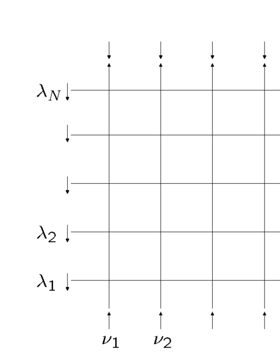
We consider the six vertex model
on a N × N 𝑁 𝑁 N\times N α 𝛼 \alpha k 𝑘 k
ℒ α k ( λ α , ν k ) subscript ℒ 𝛼 𝑘 subscript 𝜆 𝛼 subscript 𝜈 𝑘 \displaystyle\mathcal{L}_{\alpha k}(\lambda_{\alpha},\nu_{k}) = sh ( λ α − ν k + η / 2 ) R α k ( λ α − η / 2 , ν k ) absent sh subscript 𝜆 𝛼 subscript 𝜈 𝑘 𝜂 2 subscript 𝑅 𝛼 𝑘 subscript 𝜆 𝛼 𝜂 2 subscript 𝜈 𝑘 \displaystyle=\mathrm{sh}(\lambda_{\alpha}-\nu_{k}+\eta/2)R_{\alpha k}(\lambda_{\alpha}-\eta/2,\nu_{k})
= ( a ( λ α , ν k ) 0 0 0 0 b ( λ α , ν k ) c 0 0 c b ( λ α , ν k ) 0 0 0 0 a ( λ α , ν k ) ) , absent 𝑎 subscript 𝜆 𝛼 subscript 𝜈 𝑘 0 0 0 0 𝑏 subscript 𝜆 𝛼 subscript 𝜈 𝑘 𝑐 0 0 𝑐 𝑏 subscript 𝜆 𝛼 subscript 𝜈 𝑘 0 0 0 0 𝑎 subscript 𝜆 𝛼 subscript 𝜈 𝑘 \displaystyle=\left(\begin{array}[]{cccc}a(\lambda_{\alpha},\nu_{k})&0&0&0\\
0&b(\lambda_{\alpha},\nu_{k})&c&0\\
0&c&b(\lambda_{\alpha},\nu_{k})&0\\
0&0&0&a(\lambda_{\alpha},\nu_{k})\end{array}\right), (11)
where
a ( λ , ν ) = sh ( λ − ν + η / 2 ) , b ( λ , ν ) = sh ( λ − ν − η / 2 ) , c = sh η . formulae-sequence 𝑎 𝜆 𝜈 sh 𝜆 𝜈 𝜂 2 formulae-sequence 𝑏 𝜆 𝜈 sh 𝜆 𝜈 𝜂 2 𝑐 sh 𝜂 \displaystyle a(\lambda,\nu)=\mathrm{sh}(\lambda-\nu+\eta/2),\ b(\lambda,\nu)=\mathrm{sh}(\lambda-\nu-\eta/2),\ c=\mathrm{sh}\eta. (12)
We refer to the α 𝛼 \alpha 𝒱 α subscript 𝒱 𝛼 \mathcal{V}_{\alpha} k 𝑘 k ℋ k subscript ℋ 𝑘 \mathcal{H}_{k} { λ } = { λ 1 , λ 2 , … , λ N } , { ν } = { ν 1 , ν 2 , … , ν N } formulae-sequence 𝜆 subscript 𝜆 1 subscript 𝜆 2 … subscript 𝜆 𝑁 𝜈 subscript 𝜈 1 subscript 𝜈 2 … subscript 𝜈 𝑁 \{\lambda\}=\{\lambda_{1},\lambda_{2},\dots,\lambda_{N}\},\{\nu\}=\{\nu_{1},\nu_{2},\dots,\nu_{N}\} | + ⟩ , | − ⟩ ket ket
|+\rangle,|-\rangle ⟨ + | , ⟨ − | \langle+|,\langle-|
The partition function of the six vertex model, which is the summation
of products of statistical weights over all possible configurations
can be formally represented as
𝒵 N ( { λ } , { ν } ) = ⟨ + | | ⟨ − | | ∏ α , k = 1 N ℒ α k ( λ α , ν k ) | | − ⟩ a q | | + ⟩ q a , \displaystyle\mathcal{Z}_{N}(\{\lambda\},\{\nu\})={}_{a}\langle+||{}_{q}\langle-||\prod_{\alpha,k=1}^{N}\mathcal{L}_{\alpha k}(\lambda_{\alpha},\nu_{k})||-\rangle_{a}||+\rangle_{q}, (13)
where
| | + ⟩ = ⊗ k = 1 N | + ⟩ k , | | − ⟩ = ⊗ k = 1 N | − ⟩ k , ⟨ + | | = ⊗ k = 1 N ⟨ + | , ⟨ − | | = ⊗ k = 1 N ⟨ − | , k k ||+\rangle=\otimes_{k=1}^{N}|+\rangle_{k},||-\rangle=\otimes_{k=1}^{N}|-\rangle_{k},\langle+||=\otimes_{k=1}^{N}{}_{k}\langle+|,\langle-||=\otimes_{k=1}^{N}{}_{k}\langle-|, q 𝑞 q a 𝑎 a
Figure 1: The six vertex model with domain wall boundary condition.
The partition function has the following determinant form
[7 , 8 ]
𝒵 N ( { λ } , { ν } ) = ∏ α = 1 N ∏ k = 1 N a ( λ α , ν k ) b ( λ α , ν k ) det M ( { λ } , { ν } ) ∏ 1 ≤ α < β ≤ N d ( λ β , λ α ) ∏ 1 ≤ j < k ≤ N d ( ν j , ν k ) , subscript 𝒵 𝑁 𝜆 𝜈 superscript subscript product 𝛼 1 𝑁 superscript subscript product 𝑘 1 𝑁 𝑎 subscript 𝜆 𝛼 subscript 𝜈 𝑘 𝑏 subscript 𝜆 𝛼 subscript 𝜈 𝑘 𝑀 𝜆 𝜈 subscript product 1 𝛼 𝛽 𝑁 𝑑 subscript 𝜆 𝛽 subscript 𝜆 𝛼 subscript product 1 𝑗 𝑘 𝑁 𝑑 subscript 𝜈 𝑗 subscript 𝜈 𝑘 \displaystyle\mathcal{Z}_{N}(\{\lambda\},\{\nu\})=\frac{\prod_{\alpha=1}^{N}\prod_{k=1}^{N}a(\lambda_{\alpha},\nu_{k})b(\lambda_{\alpha},\nu_{k})\det M(\{\lambda\},\{\nu\})}{\prod_{1\leq\alpha<\beta\leq N}d(\lambda_{\beta},\lambda_{\alpha})\prod_{1\leq j<k\leq N}d(\nu_{j},\nu_{k})}, (14)
where
d ( λ , ν ) = sh ( λ − ν ) , M α k = φ ( λ α , ν k ) , φ ( λ , ν ) = c a ( λ , ν ) b ( λ , ν ) . formulae-sequence 𝑑 𝜆 𝜈 sh 𝜆 𝜈 formulae-sequence subscript 𝑀 𝛼 𝑘 𝜑 subscript 𝜆 𝛼 subscript 𝜈 𝑘 𝜑 𝜆 𝜈 𝑐 𝑎 𝜆 𝜈 𝑏 𝜆 𝜈 \displaystyle d(\lambda,\nu)=\mathrm{sh}(\lambda-\nu),\ M_{\alpha k}=\varphi(\lambda_{\alpha},\nu_{k}),\ \varphi(\lambda,\nu)=\frac{c}{a(\lambda,\nu)b(\lambda,\nu)}. (15)
Introducing the monodromy matrix
T α ( λ α , { ν } ) = subscript 𝑇 𝛼 subscript 𝜆 𝛼 𝜈 absent \displaystyle T_{\alpha}(\lambda_{\alpha},\{\nu\})= ℒ α N ( λ α , ν N ) ⋯ ℒ α 1 ( λ α , ν 1 ) subscript ℒ 𝛼 𝑁 subscript 𝜆 𝛼 subscript 𝜈 𝑁 ⋯ subscript ℒ 𝛼 1 subscript 𝜆 𝛼 subscript 𝜈 1 \displaystyle\mathcal{L}_{\alpha N}(\lambda_{\alpha},\nu_{N})\cdots\mathcal{L}_{\alpha 1}(\lambda_{\alpha},\nu_{1})
= \displaystyle= ( A ( λ α , { ν } ) B ( λ α , { ν } ) C ( λ α , { ν } ) D ( λ α , { ν } ) ) , 𝐴 subscript 𝜆 𝛼 𝜈 𝐵 subscript 𝜆 𝛼 𝜈 𝐶 subscript 𝜆 𝛼 𝜈 𝐷 subscript 𝜆 𝛼 𝜈 \displaystyle\left(\begin{array}[]{cc}A(\lambda_{\alpha},\{\nu\})&B(\lambda_{\alpha},\{\nu\})\\
C(\lambda_{\alpha},\{\nu\})&D(\lambda_{\alpha},\{\nu\})\end{array}\right), (18)
the partition function can be represented as
𝒵 N ( { λ } , { ν } ) = ⟨ − | | B ( λ N , { ν } ) ⋯ B ( λ 1 , { ν } ) | | + ⟩ q q \displaystyle\mathcal{Z}_{N}(\{\lambda\},\{\nu\})={}_{q}\langle-||B(\lambda_{N},\{\nu\})\cdots B(\lambda_{1},\{\nu\})||+\rangle_{q}\, (19)
From the Yang-Baxter equation, one has
R α β ( μ − λ ) T α ( μ , { ν } ) T β ( λ , { ν } ) = T β ( λ , { ν } ) T α ( μ , { ν } ) R α β ( μ − λ ) . subscript 𝑅 𝛼 𝛽 𝜇 𝜆 subscript 𝑇 𝛼 𝜇 𝜈 subscript 𝑇 𝛽 𝜆 𝜈 subscript 𝑇 𝛽 𝜆 𝜈 subscript 𝑇 𝛼 𝜇 𝜈 subscript 𝑅 𝛼 𝛽 𝜇 𝜆 \displaystyle R_{\alpha\beta}(\mu-\lambda)T_{\alpha}(\mu,\{\nu\})T_{\beta}(\lambda,\{\nu\})=T_{\beta}(\lambda,\{\nu\})T_{\alpha}(\mu,\{\nu\})R_{\alpha\beta}(\mu-\lambda). (20)
From (20
A ( λ , { ν } ) B ( μ , { ν } ) 𝐴 𝜆 𝜈 𝐵 𝜇 𝜈 \displaystyle A(\lambda,\{\nu\})B(\mu,\{\nu\}) = f ( λ , μ ) B ( μ , { ν } ) A ( λ , { ν } ) + g ( μ , λ ) B ( λ , { ν } ) A ( μ , { ν } ) , absent 𝑓 𝜆 𝜇 𝐵 𝜇 𝜈 𝐴 𝜆 𝜈 𝑔 𝜇 𝜆 𝐵 𝜆 𝜈 𝐴 𝜇 𝜈 \displaystyle=f(\lambda,\mu)B(\mu,\{\nu\})A(\lambda,\{\nu\})+g(\mu,\lambda)B(\lambda,\{\nu\})A(\mu,\{\nu\}), (21)
B ( λ , { ν } ) A ( μ , { ν } ) 𝐵 𝜆 𝜈 𝐴 𝜇 𝜈 \displaystyle B(\lambda,\{\nu\})A(\mu,\{\nu\}) = f ( λ , μ ) A ( μ , { ν } ) B ( λ , { ν } ) + g ( μ , λ ) A ( λ , { ν } ) B ( μ , { ν } ) , absent 𝑓 𝜆 𝜇 𝐴 𝜇 𝜈 𝐵 𝜆 𝜈 𝑔 𝜇 𝜆 𝐴 𝜆 𝜈 𝐵 𝜇 𝜈 \displaystyle=f(\lambda,\mu)A(\mu,\{\nu\})B(\lambda,\{\nu\})+g(\mu,\lambda)A(\lambda,\{\nu\})B(\mu,\{\nu\}), (22)
B ( λ , { ν } ) B ( μ , { ν } ) 𝐵 𝜆 𝜈 𝐵 𝜇 𝜈 \displaystyle B(\lambda,\{\nu\})B(\mu,\{\nu\}) = B ( μ , { ν } ) B ( λ , { ν } ) , absent 𝐵 𝜇 𝜈 𝐵 𝜆 𝜈 \displaystyle=B(\mu,\{\nu\})B(\lambda,\{\nu\}), (23)
where
f ( μ , λ ) = sh ( λ − μ + η ) sh ( λ − μ ) , g ( μ , λ ) = sh η sh ( λ − μ ) , formulae-sequence 𝑓 𝜇 𝜆 sh 𝜆 𝜇 𝜂 sh 𝜆 𝜇 𝑔 𝜇 𝜆 sh 𝜂 sh 𝜆 𝜇 \displaystyle f(\mu,\lambda)=\frac{\mathrm{sh}(\lambda-\mu+\eta)}{\mathrm{sh}(\lambda-\mu)},\ g(\mu,\lambda)=\frac{\mathrm{sh}\eta}{\mathrm{sh}(\lambda-\mu)}, (24)
for example.
3 Boundary correlation functions of the six vertex model
In this section, we consider the following
boundary correlation functions
ℱ N ( r , ϵ 1 , ⋯ , ϵ s ) ( { λ } , { ν } ) superscript subscript ℱ 𝑁 𝑟 subscript italic-ϵ 1 ⋯ subscript italic-ϵ 𝑠 𝜆 𝜈 \displaystyle\mathcal{F}_{N}^{(r,\epsilon_{1},\cdots,\epsilon_{s})}(\{\lambda\},\{\nu\}) = ℱ ~ N ( r , ϵ 1 , ⋯ , ϵ s ) ( { λ } , { ν } ) 𝒵 N ( { λ } , { ν } ) , absent superscript subscript ~ ℱ 𝑁 𝑟 subscript italic-ϵ 1 ⋯ subscript italic-ϵ 𝑠 𝜆 𝜈 subscript 𝒵 𝑁 𝜆 𝜈 \displaystyle=\frac{\widetilde{\mathcal{F}}_{N}^{(r,\epsilon_{1},\cdots,\epsilon_{s})}(\{\lambda\},\{\nu\})}{\mathcal{Z}_{N}(\{\lambda\},\{\nu\})}, (25)
ℱ ~ N ( r , ϵ 1 , ⋯ , ϵ s ) ( { λ } , { ν } ) superscript subscript ~ ℱ 𝑁 𝑟 subscript italic-ϵ 1 ⋯ subscript italic-ϵ 𝑠 𝜆 𝜈 \displaystyle\widetilde{\mathcal{F}}_{N}^{(r,\epsilon_{1},\cdots,\epsilon_{s})}(\{\lambda\},\{\nu\}) = ⟨ + | | ⟨ − | | ∏ α = r + 1 N ∏ k = 1 N ℒ α k ( λ α , ν k ) ∏ k = 1 s π k ϵ k ∏ α = 1 r ∏ k = 1 N ℒ α k ( λ α , ν k ) | | − ⟩ a q | | + ⟩ q a , \displaystyle={}_{a}\langle+||{}_{q}\langle-||\prod_{\alpha=r+1}^{N}\prod_{k=1}^{N}\mathcal{L}_{\alpha k}(\lambda_{\alpha},\nu_{k})\prod_{k=1}^{s}\pi_{k}^{\epsilon_{k}}\prod_{\alpha=1}^{r}\prod_{k=1}^{N}\mathcal{L}_{\alpha k}(\lambda_{\alpha},\nu_{k})||-\rangle_{a}||+\rangle_{q}, (26)
where π k + = | + ⟩ k k ⟨ + | \pi_{k}^{+}=|+\rangle_{k}{}_{k}\langle+| π k − = | − ⟩ k k ⟨ − | \pi_{k}^{-}=|-\rangle_{k}{}_{k}\langle-| [25 , 26 , 27 , 28 , 29 ] .
We calculate the boundary correlation functions
by use of the quantum inverse scattering method,
applying the approach of [29 ] .
Figure 2: An example of boundary correlation function.
First,
note that (26
ℱ ~ N ( r , ϵ 1 , ⋯ , ϵ s ) ( { λ } , { ν } ) = ⟨ − | | B ( λ N , { ν } ) ⋯ B ( λ r + 1 , { ν } ) ∏ k = 1 s π k ϵ k B ( λ r , { ν } ) ⋯ B ( λ 1 , { ν } ) | | + ⟩ q q , \displaystyle\widetilde{\mathcal{F}}_{N}^{(r,\epsilon_{1},\cdots,\epsilon_{s})}(\{\lambda\},\{\nu\})={}_{q}\langle-||B(\lambda_{N},\{\nu\})\cdots B(\lambda_{r+1},\{\nu\})\prod_{k=1}^{s}\pi_{k}^{\epsilon_{k}}B(\lambda_{r},\{\nu\})\cdots B(\lambda_{1},\{\nu\})||+\rangle_{q}, (27)
in the quantum inverse scattering language.
We introduce the following two-site model [10 ]
in order to obtain recursive relations between boundary
correlation functions of different lattice sizes.
T ( λ , { ν } ) = 𝑇 𝜆 𝜈 absent \displaystyle T(\lambda,\{\nu\})= T 2 ( λ , { ν } \ ν 1 ) T 1 ( λ , ν 1 ) subscript 𝑇 2 𝜆 \ 𝜈 subscript 𝜈 1 subscript 𝑇 1 𝜆 subscript 𝜈 1 \displaystyle T_{2}(\lambda,\{\nu\}\backslash\nu_{1})T_{1}(\lambda,\nu_{1}) (28)
T 2 ( λ , { ν } \ ν 1 ) = subscript 𝑇 2 𝜆 \ 𝜈 subscript 𝜈 1 absent \displaystyle T_{2}(\lambda,\{\nu\}\backslash\nu_{1})= ℒ α N ( λ , ν N ) ⋯ ℒ α 2 ( λ , ν 2 ) subscript ℒ 𝛼 𝑁 𝜆 subscript 𝜈 𝑁 ⋯ subscript ℒ 𝛼 2 𝜆 subscript 𝜈 2 \displaystyle\mathcal{L}_{\alpha N}(\lambda,\nu_{N})\cdots\mathcal{L}_{\alpha 2}(\lambda,\nu_{2})
= \displaystyle= ( A 2 ( λ , { ν } \ ν 1 ) B 2 ( λ , { ν } \ ν 1 ) C 2 ( λ , { ν } \ ν 1 ) D 2 ( λ , { ν } \ ν 1 ) ) , subscript 𝐴 2 𝜆 \ 𝜈 subscript 𝜈 1 subscript 𝐵 2 𝜆 \ 𝜈 subscript 𝜈 1 subscript 𝐶 2 𝜆 \ 𝜈 subscript 𝜈 1 subscript 𝐷 2 𝜆 \ 𝜈 subscript 𝜈 1 \displaystyle\left(\begin{array}[]{cc}A_{2}(\lambda,\{\nu\}\backslash\nu_{1})&B_{2}(\lambda,\{\nu\}\backslash\nu_{1})\\
C_{2}(\lambda,\{\nu\}\backslash\nu_{1})&D_{2}(\lambda,\{\nu\}\backslash\nu_{1})\end{array}\right), (31)
T 1 ( λ , ν 1 ) = subscript 𝑇 1 𝜆 subscript 𝜈 1 absent \displaystyle T_{1}(\lambda,\nu_{1})= ℒ α 1 ( λ , ν 1 ) . subscript ℒ 𝛼 1 𝜆 subscript 𝜈 1 \displaystyle\mathcal{L}_{\alpha 1}(\lambda,\nu_{1}). (32)
Applying
⟨ + | B ( λ , { ν } ) | + ⟩ 1 1 \displaystyle{}_{1}\langle+|B(\lambda,\{\nu\})|+\rangle_{1} = b ( λ , ν 1 ) B 2 ( λ , { ν } \ ν 1 ) , absent 𝑏 𝜆 subscript 𝜈 1 subscript 𝐵 2 𝜆 \ 𝜈 subscript 𝜈 1 \displaystyle=b(\lambda,\nu_{1})B_{2}(\lambda,\{\nu\}\backslash\nu_{1}),
⟨ − | B ( λ , { ν } ) | + ⟩ 1 1 \displaystyle{}_{1}\langle-|B(\lambda,\{\nu\})|+\rangle_{1} = c A 2 ( λ , { ν } \ ν 1 ) , absent 𝑐 subscript 𝐴 2 𝜆 \ 𝜈 subscript 𝜈 1 \displaystyle=cA_{2}(\lambda,\{\nu\}\backslash\nu_{1}),
⟨ + | B ( λ , { ν } ) | − ⟩ 1 1 \displaystyle{}_{1}\langle+|B(\lambda,\{\nu\})|-\rangle_{1} = 0 , absent 0 \displaystyle=0,
⟨ − | B ( λ , { ν } ) | − ⟩ 1 1 \displaystyle{}_{1}\langle-|B(\lambda,\{\nu\})|-\rangle_{1} = a ( λ , ν 1 ) B 2 ( λ , { ν } \ ν 1 ) , absent 𝑎 𝜆 subscript 𝜈 1 subscript 𝐵 2 𝜆 \ 𝜈 subscript 𝜈 1 \displaystyle=a(\lambda,\nu_{1})B_{2}(\lambda,\{\nu\}\backslash\nu_{1}), (33)
iteratively, one has
⟨ + | B ( λ n , { ν } ) ⋯ B ( λ 1 , { ν } ) | + ⟩ 1 1 = ∏ j = 1 n b ( λ j , ν 1 ) B 2 ( λ n , { ν } \ ν 1 ) ⋯ B 2 ( λ 1 , { ν } \ ν 1 ) , \displaystyle{}_{1}\langle+|B(\lambda_{n},\{\nu\})\cdots B(\lambda_{1},\{\nu\})|+\rangle_{1}=\prod_{j=1}^{n}b(\lambda_{j},\nu_{1})B_{2}(\lambda_{n},\{\nu\}\backslash\nu_{1})\cdots B_{2}(\lambda_{1},\{\nu\}\backslash\nu_{1}), (34)
⟨ − | B ( λ n , { ν } ) ⋯ B ( λ 1 , { ν } ) | − ⟩ 1 1 = ∏ j = 1 n a ( λ j , ν 1 ) B 2 ( λ n , { ν } \ ν 1 ) ⋯ B 2 ( λ 1 , { ν } \ ν 1 ) , \displaystyle{}_{1}\langle-|B(\lambda_{n},\{\nu\})\cdots B(\lambda_{1},\{\nu\})|-\rangle_{1}=\prod_{j=1}^{n}a(\lambda_{j},\nu_{1})B_{2}(\lambda_{n},\{\nu\}\backslash\nu_{1})\cdots B_{2}(\lambda_{1},\{\nu\}\backslash\nu_{1}), (35)
⟨ − | B ( λ n , { ν } ) ⋯ B ( λ 1 , { ν } ) | + ⟩ 1 1 \displaystyle{}_{1}\langle-|B(\lambda_{n},\{\nu\})\cdots B(\lambda_{1},\{\nu\})|+\rangle_{1}
= \displaystyle= ∑ α = 1 n ∏ β = α + 1 n a ( λ β , ν 1 ) c ∏ β = 1 α − 1 b ( λ β , ν 1 ) B 2 ( λ n , { ν } \ ν 1 ) ⋯ B 2 ( λ α + 1 , { ν } \ ν 1 ) superscript subscript 𝛼 1 𝑛 superscript subscript product 𝛽 𝛼 1 𝑛 𝑎 subscript 𝜆 𝛽 subscript 𝜈 1 𝑐 superscript subscript product 𝛽 1 𝛼 1 𝑏 subscript 𝜆 𝛽 subscript 𝜈 1 subscript 𝐵 2 subscript 𝜆 𝑛 \ 𝜈 subscript 𝜈 1 ⋯ subscript 𝐵 2 subscript 𝜆 𝛼 1 \ 𝜈 subscript 𝜈 1 \displaystyle\sum_{\alpha=1}^{n}\prod_{\beta=\alpha+1}^{n}a(\lambda_{\beta},\nu_{1})c\prod_{\beta=1}^{\alpha-1}b(\lambda_{\beta},\nu_{1})B_{2}(\lambda_{n},\{\nu\}\backslash\nu_{1})\cdots B_{2}(\lambda_{\alpha+1},\{\nu\}\backslash\nu_{1})
× A 2 ( λ α , { ν } \ ν 1 ) B 2 ( λ α − 1 , { ν } \ ν 1 ) ⋯ B 2 ( λ 1 , { ν } \ ν 1 ) . absent subscript 𝐴 2 subscript 𝜆 𝛼 \ 𝜈 subscript 𝜈 1 subscript 𝐵 2 subscript 𝜆 𝛼 1 \ 𝜈 subscript 𝜈 1 ⋯ subscript 𝐵 2 subscript 𝜆 1 \ 𝜈 subscript 𝜈 1 \displaystyle\times A_{2}(\lambda_{\alpha},\{\nu\}\backslash\nu_{1})B_{2}(\lambda_{\alpha-1},\{\nu\}\backslash\nu_{1})\cdots B_{2}(\lambda_{1},\{\nu\}\backslash\nu_{1}). (36)
Combining (36
A 2 ( λ , { ν } \ ν 1 ) B 2 ( μ , { ν } \ ν 1 ) = subscript 𝐴 2 𝜆 \ 𝜈 subscript 𝜈 1 subscript 𝐵 2 𝜇 \ 𝜈 subscript 𝜈 1 absent \displaystyle A_{2}(\lambda,\{\nu\}\backslash\nu_{1})B_{2}(\mu,\{\nu\}\backslash\nu_{1})= f ( λ , μ ) B 2 ( μ , { ν } \ ν 1 ) A 2 ( λ , { ν } \ ν 1 ) 𝑓 𝜆 𝜇 subscript 𝐵 2 𝜇 \ 𝜈 subscript 𝜈 1 subscript 𝐴 2 𝜆 \ 𝜈 subscript 𝜈 1 \displaystyle f(\lambda,\mu)B_{2}(\mu,\{\nu\}\backslash\nu_{1})A_{2}(\lambda,\{\nu\}\backslash\nu_{1})
+ g ( μ , λ ) B 2 ( λ , { ν } \ ν 1 ) A 2 ( μ , { ν } \ ν 1 ) , 𝑔 𝜇 𝜆 subscript 𝐵 2 𝜆 \ 𝜈 subscript 𝜈 1 subscript 𝐴 2 𝜇 \ 𝜈 subscript 𝜈 1 \displaystyle+g(\mu,\lambda)B_{2}(\lambda,\{\nu\}\backslash\nu_{1})A_{2}(\mu,\{\nu\}\backslash\nu_{1}), (37)
and
A 2 ( λ , { ν } \ ν 1 ) ⊗ k = 2 N | + ⟩ k = ∏ k = 2 N a ( λ , ν k ) ⊗ k = 2 N | + ⟩ k , superscript subscript tensor-product 𝑘 2 𝑁 subscript 𝐴 2 𝜆 \ 𝜈 subscript 𝜈 1 subscript ket 𝑘 superscript subscript product 𝑘 2 𝑁 superscript subscript tensor-product 𝑘 2 𝑁 𝑎 𝜆 subscript 𝜈 𝑘 subscript ket 𝑘 \displaystyle A_{2}(\lambda,\{\nu\}\backslash\nu_{1})\otimes_{k=2}^{N}|+\rangle_{k}=\prod_{k=2}^{N}a(\lambda,\nu_{k})\otimes_{k=2}^{N}|+\rangle_{k}, (38)
we get
⟨ − | B ( λ r , { ν } ) ⋯ B ( λ 1 , { ν } ) | | + ⟩ 1 \displaystyle{}_{1}\langle-|B(\lambda_{r},\{\nu\})\cdots B(\lambda_{1},\{\nu\})||+\rangle
= \displaystyle= ∑ α = 1 r c ∏ β = 1 β ≠ α r b ( λ β , ν 1 ) ∏ β = 1 β ≠ α r f ( λ α , λ β ) ∏ k = 2 N a ( λ α , ν k ) ∏ k = 1 k ≠ α r B 2 ( λ k , { ν } \ ν 1 ) ⊗ k = 2 N | + ⟩ k . superscript subscript 𝛼 1 𝑟 𝑐 superscript subscript product 𝛽 1 𝛽 𝛼
𝑟 𝑏 subscript 𝜆 𝛽 subscript 𝜈 1 superscript subscript product 𝛽 1 𝛽 𝛼
𝑟 𝑓 subscript 𝜆 𝛼 subscript 𝜆 𝛽 superscript subscript product 𝑘 2 𝑁 𝑎 subscript 𝜆 𝛼 subscript 𝜈 𝑘 superscript subscript product 𝑘 1 𝑘 𝛼
𝑟 superscript subscript tensor-product 𝑘 2 𝑁 subscript 𝐵 2 subscript 𝜆 𝑘 \ 𝜈 subscript 𝜈 1 subscript ket 𝑘 \displaystyle\sum_{\alpha=1}^{r}c\prod_{\begin{subarray}{c}\beta=1\\
\beta\neq\alpha\end{subarray}}^{r}b(\lambda_{\beta},\nu_{1})\prod_{\begin{subarray}{c}\beta=1\\
\beta\neq\alpha\end{subarray}}^{r}f(\lambda_{\alpha},\lambda_{\beta})\prod_{k=2}^{N}a(\lambda_{\alpha},\nu_{k})\prod_{\begin{subarray}{c}k=1\\
k\neq\alpha\end{subarray}}^{r}B_{2}(\lambda_{k},\{\nu\}\backslash\nu_{1})\otimes_{k=2}^{N}|+\rangle_{k}. (39)
In the same way as (39
⟨ − | | B ( λ N , { ν } ) ⋯ B ( λ r + 1 , { ν } ) | + ⟩ 1 \displaystyle\langle-||B(\lambda_{N},\{\nu\})\cdots B(\lambda_{r+1},\{\nu\})|+\rangle_{1}
= \displaystyle= ∑ α = r + 1 N c ∏ β = r + 1 β ≠ α N a ( λ β , ν 1 ) ∏ β = r + 1 β ≠ α N f ( λ β , λ α ) ∏ k = 2 N b ( λ α , ν k ) ⊗ k = 2 N ⟨ − | ∏ k = r + 1 k ≠ α N B 2 ( λ k , { ν } \ ν 1 ) , k \displaystyle\sum_{\alpha=r+1}^{N}c\prod_{\begin{subarray}{c}\beta=r+1\\
\beta\neq\alpha\end{subarray}}^{N}a(\lambda_{\beta},\nu_{1})\prod_{\begin{subarray}{c}\beta=r+1\\
\beta\neq\alpha\end{subarray}}^{N}f(\lambda_{\beta},\lambda_{\alpha})\prod_{k=2}^{N}b(\lambda_{\alpha},\nu_{k})\otimes_{k=2}^{N}{}_{k}\langle-|\prod_{\begin{subarray}{c}k=r+1\\
k\neq\alpha\end{subarray}}^{N}B_{2}(\lambda_{k},\{\nu\}\backslash\nu_{1}), (40)
utilizing
(36
B 2 ( λ , { ν } \ ν 1 ) A 2 ( μ , { ν } \ ν 1 ) = subscript 𝐵 2 𝜆 \ 𝜈 subscript 𝜈 1 subscript 𝐴 2 𝜇 \ 𝜈 subscript 𝜈 1 absent \displaystyle B_{2}(\lambda,\{\nu\}\backslash\nu_{1})A_{2}(\mu,\{\nu\}\backslash\nu_{1})= f ( λ , μ ) A 2 ( μ , { ν } \ ν 1 ) B 2 ( λ , { ν } \ ν 1 ) 𝑓 𝜆 𝜇 subscript 𝐴 2 𝜇 \ 𝜈 subscript 𝜈 1 subscript 𝐵 2 𝜆 \ 𝜈 subscript 𝜈 1 \displaystyle f(\lambda,\mu)A_{2}(\mu,\{\nu\}\backslash\nu_{1})B_{2}(\lambda,\{\nu\}\backslash\nu_{1})
+ g ( μ , λ ) A 2 ( λ , { ν } \ ν 1 ) B 2 ( μ , { ν } \ ν 1 ) , 𝑔 𝜇 𝜆 subscript 𝐴 2 𝜆 \ 𝜈 subscript 𝜈 1 subscript 𝐵 2 𝜇 \ 𝜈 subscript 𝜈 1 \displaystyle+g(\mu,\lambda)A_{2}(\lambda,\{\nu\}\backslash\nu_{1})B_{2}(\mu,\{\nu\}\backslash\nu_{1}), (41)
and
⊗ k = 2 N ⟨ − | A 2 ( λ , { ν } \ ν 1 ) = ∏ k = 2 N b ( λ , ν k ) ⊗ k = 2 N ⟨ − | . k k \displaystyle\otimes_{k=2}^{N}{}_{k}\langle-|A_{2}(\lambda,\{\nu\}\backslash\nu_{1})=\prod_{k=2}^{N}b(\lambda,\nu_{k})\otimes_{k=2}^{N}{}_{k}\langle-|. (42)
From
(35 39 [29 ]
ℱ N ( r , − , ϵ 2 , ⋯ , ϵ s ) ( { λ } , { ν } ) = superscript subscript ℱ 𝑁 𝑟 subscript italic-ϵ 2 ⋯ subscript italic-ϵ 𝑠 𝜆 𝜈 absent \displaystyle\mathcal{F}_{N}^{(r,-,\epsilon_{2},\cdots,\epsilon_{s})}(\{\lambda\},\{\nu\})= ∏ β = r + 1 N a ( λ β , ν 1 ) ∑ α = 1 r c ∏ β = 1 β ≠ α r b ( λ β , ν 1 ) ∏ β = 1 β ≠ α r f ( λ α , λ β ) ∏ k = 2 N a ( λ α , ν k ) superscript subscript product 𝛽 𝑟 1 𝑁 𝑎 subscript 𝜆 𝛽 subscript 𝜈 1 superscript subscript 𝛼 1 𝑟 𝑐 superscript subscript product 𝛽 1 𝛽 𝛼
𝑟 𝑏 subscript 𝜆 𝛽 subscript 𝜈 1 superscript subscript product 𝛽 1 𝛽 𝛼
𝑟 𝑓 subscript 𝜆 𝛼 subscript 𝜆 𝛽 superscript subscript product 𝑘 2 𝑁 𝑎 subscript 𝜆 𝛼 subscript 𝜈 𝑘 \displaystyle\prod_{\beta=r+1}^{N}a(\lambda_{\beta},\nu_{1})\sum_{\alpha=1}^{r}c\prod_{\begin{subarray}{c}\beta=1\\
\beta\neq\alpha\end{subarray}}^{r}b(\lambda_{\beta},\nu_{1})\prod_{\begin{subarray}{c}\beta=1\\
\beta\neq\alpha\end{subarray}}^{r}f(\lambda_{\alpha},\lambda_{\beta})\prod_{k=2}^{N}a(\lambda_{\alpha},\nu_{k})
× ℱ N − 1 ( r − 1 , ϵ 2 , ⋯ , ϵ s ) ( { λ } \ λ α , { ν } \ ν 1 ) . absent superscript subscript ℱ 𝑁 1 𝑟 1 subscript italic-ϵ 2 ⋯ subscript italic-ϵ 𝑠 \ 𝜆 subscript 𝜆 𝛼 \ 𝜈 subscript 𝜈 1 \displaystyle\times\mathcal{F}_{N-1}^{(r-1,\epsilon_{2},\cdots,\epsilon_{s})}(\{\lambda\}\backslash\lambda_{\alpha},\{\nu\}\backslash\nu_{1}). (43)
We can obtain another recursive relation
from (34 40
ℱ N ( r , + , ϵ 2 , ⋯ , ϵ s ) ( { λ } , { ν } ) = superscript subscript ℱ 𝑁 𝑟 subscript italic-ϵ 2 ⋯ subscript italic-ϵ 𝑠 𝜆 𝜈 absent \displaystyle\mathcal{F}_{N}^{(r,+,\epsilon_{2},\cdots,\epsilon_{s})}(\{\lambda\},\{\nu\})= ∏ β = 1 r b ( λ β , ν 1 ) ∑ α = r + 1 N c ∏ β = r + 1 β ≠ α N a ( λ β , ν 1 ) ∏ β = r + 1 β ≠ α N f ( λ β , λ α ) ∏ k = 2 N b ( λ α , ν k ) superscript subscript product 𝛽 1 𝑟 𝑏 subscript 𝜆 𝛽 subscript 𝜈 1 superscript subscript 𝛼 𝑟 1 𝑁 𝑐 superscript subscript product 𝛽 𝑟 1 𝛽 𝛼
𝑁 𝑎 subscript 𝜆 𝛽 subscript 𝜈 1 superscript subscript product 𝛽 𝑟 1 𝛽 𝛼
𝑁 𝑓 subscript 𝜆 𝛽 subscript 𝜆 𝛼 superscript subscript product 𝑘 2 𝑁 𝑏 subscript 𝜆 𝛼 subscript 𝜈 𝑘 \displaystyle\prod_{\beta=1}^{r}b(\lambda_{\beta},\nu_{1})\sum_{\alpha=r+1}^{N}c\prod_{\begin{subarray}{c}\beta=r+1\\
\beta\neq\alpha\end{subarray}}^{N}a(\lambda_{\beta},\nu_{1})\prod_{\begin{subarray}{c}\beta=r+1\\
\beta\neq\alpha\end{subarray}}^{N}f(\lambda_{\beta},\lambda_{\alpha})\prod_{k=2}^{N}b(\lambda_{\alpha},\nu_{k})
× ℱ N − 1 ( r , ϵ 2 , ⋯ , ϵ s ) ( { λ } \ λ α , { ν } \ ν 1 ) . absent superscript subscript ℱ 𝑁 1 𝑟 subscript italic-ϵ 2 ⋯ subscript italic-ϵ 𝑠 \ 𝜆 subscript 𝜆 𝛼 \ 𝜈 subscript 𝜈 1 \displaystyle\times\mathcal{F}_{N-1}^{(r,\epsilon_{2},\cdots,\epsilon_{s})}(\{\lambda\}\backslash\lambda_{\alpha},\{\nu\}\backslash\nu_{1}). (44)
Solving these two recursive relations
(43 44
ℱ N ( r , ϵ 1 , ⋯ , ϵ s ) ( { λ } , { ν } ) superscript subscript ℱ 𝑁 𝑟 subscript italic-ϵ 1 ⋯ subscript italic-ϵ 𝑠 𝜆 𝜈 \displaystyle\mathcal{F}_{N}^{(r,\epsilon_{1},\cdots,\epsilon_{s})}(\{\lambda\},\{\nu\})
= \displaystyle= 1 det M ( { λ } , { ν } ) ∏ j = 1 s ∏ k = j + 1 N d ( ν j , ν k ) ∏ β = 1 r a ( λ β , ν j ) ∏ β = r + 1 N b ( λ β , ν j ) ∑ α 1 ∈ S ϵ 1 N , r ∑ α 2 ∈ S ϵ 2 N , r α 2 ≠ α 1 ⋯ ∑ α s ∈ S ϵ s N , r α s ≠ α 1 , ⋯ , α s − 1 1 𝑀 𝜆 𝜈 superscript subscript product 𝑗 1 𝑠 superscript subscript product 𝑘 𝑗 1 𝑁 𝑑 subscript 𝜈 𝑗 subscript 𝜈 𝑘 superscript subscript product 𝛽 1 𝑟 𝑎 subscript 𝜆 𝛽 subscript 𝜈 𝑗 superscript subscript product 𝛽 𝑟 1 𝑁 𝑏 subscript 𝜆 𝛽 subscript 𝜈 𝑗 subscript subscript 𝛼 1 superscript subscript 𝑆 subscript italic-ϵ 1 𝑁 𝑟
subscript subscript 𝛼 2 superscript subscript 𝑆 subscript italic-ϵ 2 𝑁 𝑟
subscript 𝛼 2 subscript 𝛼 1
⋯ subscript subscript 𝛼 𝑠 superscript subscript 𝑆 subscript italic-ϵ 𝑠 𝑁 𝑟
subscript 𝛼 𝑠 subscript 𝛼 1 ⋯ subscript 𝛼 𝑠 1
\displaystyle\frac{1}{\det M(\{\lambda\},\{\nu\})}\prod_{j=1}^{s}\frac{\prod_{k=j+1}^{N}d(\nu_{j},\nu_{k})}{\prod_{\beta=1}^{r}a(\lambda_{\beta},\nu_{j})\prod_{\beta=r+1}^{N}b(\lambda_{\beta},\nu_{j})}\sum_{\alpha_{1}\in S_{\epsilon_{1}}^{N,r}}\sum_{\begin{subarray}{c}\alpha_{2}\in S_{\epsilon_{2}}^{N,r}\\
\alpha_{2}\neq\alpha_{1}\end{subarray}}\cdots\sum_{\begin{subarray}{c}\alpha_{s}\in S_{\epsilon_{s}}^{N,r}\\
\alpha_{s}\neq\alpha_{1},\cdots,\alpha_{s-1}\end{subarray}}
× ( − 1 ) ∑ 1 ≤ j < k ≤ s χ ( α k , α j ) + ∑ k = 1 s ( α k − 1 − r ( ϵ k + 1 ) / 2 ) + ∑ k = 1 s ( ϵ k + 1 ) ( N − k ) / 2 absent superscript 1 subscript 1 𝑗 𝑘 𝑠 𝜒 subscript 𝛼 𝑘 subscript 𝛼 𝑗 superscript subscript 𝑘 1 𝑠 subscript 𝛼 𝑘 1 𝑟 subscript italic-ϵ 𝑘 1 2 superscript subscript 𝑘 1 𝑠 subscript italic-ϵ 𝑘 1 𝑁 𝑘 2 \displaystyle\times(-1)^{\sum_{1\leq j<k\leq s}\chi(\alpha_{k},\alpha_{j})+\sum_{k=1}^{s}(\alpha_{k}-1-r(\epsilon_{k}+1)/2)+\sum_{k=1}^{s}(\epsilon_{k}+1)(N-k)/2}
× ∏ j = 1 s H r ϵ j ( λ α j ) ∏ 1 ≤ j < k ≤ s E ϵ j ϵ k ( λ α j , λ α k , ν j , ν k ) det M ( { λ } \ { λ α 1 , ⋯ , λ α s } , { ν } \ { ν 1 , ⋯ , ν s } ) , \displaystyle\times\prod_{j=1}^{s}H_{r}^{\epsilon_{j}}(\lambda_{\alpha_{j}})\prod_{1\leq j<k\leq s}E^{\epsilon_{j}\epsilon_{k}}(\lambda_{\alpha_{j}},\lambda_{\alpha_{k}},\nu_{j},\nu_{k})\det M(\{\lambda\}\backslash\{\lambda_{\alpha_{1}},\cdots,\lambda_{\alpha_{s}}\},\{\nu\}\backslash\{\nu_{1},\cdots,\nu_{s}\}), (45)
where
S − N , r = { 1 , ⋯ , r } , S + N , r = { r + 1 , ⋯ , N } , e ( λ , ν ) = sh ( λ − ν + η ) formulae-sequence superscript subscript 𝑆 𝑁 𝑟
1 ⋯ 𝑟 formulae-sequence superscript subscript 𝑆 𝑁 𝑟
𝑟 1 ⋯ 𝑁 𝑒 𝜆 𝜈 sh 𝜆 𝜈 𝜂 S_{-}^{N,r}=\{1,\cdots,r\},S_{+}^{N,r}=\{r+1,\cdots,N\},e(\lambda,\nu)=\mathrm{sh}(\lambda-\nu+\eta)
H r − ( λ ) = ∏ β = 1 r e ( λ β , λ ) ∏ β = r + 1 N d ( λ β , λ ) ∏ k = 1 N b ( λ , ν k ) , superscript subscript 𝐻 𝑟 𝜆 superscript subscript product 𝛽 1 𝑟 𝑒 subscript 𝜆 𝛽 𝜆 superscript subscript product 𝛽 𝑟 1 𝑁 𝑑 subscript 𝜆 𝛽 𝜆 superscript subscript product 𝑘 1 𝑁 𝑏 𝜆 subscript 𝜈 𝑘 \displaystyle H_{r}^{-}(\lambda)=\frac{\prod_{\beta=1}^{r}e(\lambda_{\beta},\lambda)\prod_{\beta=r+1}^{N}d(\lambda_{\beta},\lambda)}{\prod_{k=1}^{N}b(\lambda,\nu_{k})}, (46)
H r + ( λ ) = ∏ β = 1 r d ( λ β , λ ) ∏ β = r + 1 N e ( λ , λ β ) ∏ k = 1 N a ( λ , ν k ) , superscript subscript 𝐻 𝑟 𝜆 superscript subscript product 𝛽 1 𝑟 𝑑 subscript 𝜆 𝛽 𝜆 superscript subscript product 𝛽 𝑟 1 𝑁 𝑒 𝜆 subscript 𝜆 𝛽 superscript subscript product 𝑘 1 𝑁 𝑎 𝜆 subscript 𝜈 𝑘 \displaystyle H_{r}^{+}(\lambda)=\frac{\prod_{\beta=1}^{r}d(\lambda_{\beta},\lambda)\prod_{\beta=r+1}^{N}e(\lambda,\lambda_{\beta})}{\prod_{k=1}^{N}a(\lambda,\nu_{k})}, (47)
E − + ( λ α j , λ α k , ν j , ν k ) = a ( λ α j , ν k ) a ( λ α k , ν j ) d ( λ α j , λ α k ) , superscript 𝐸 absent subscript 𝜆 subscript 𝛼 𝑗 subscript 𝜆 subscript 𝛼 𝑘 subscript 𝜈 𝑗 subscript 𝜈 𝑘 𝑎 subscript 𝜆 subscript 𝛼 𝑗 subscript 𝜈 𝑘 𝑎 subscript 𝜆 subscript 𝛼 𝑘 subscript 𝜈 𝑗 𝑑 subscript 𝜆 subscript 𝛼 𝑗 subscript 𝜆 subscript 𝛼 𝑘 \displaystyle E^{-+}(\lambda_{\alpha_{j}},\lambda_{\alpha_{k}},\nu_{j},\nu_{k})=\frac{a(\lambda_{\alpha_{j}},\nu_{k})a(\lambda_{\alpha_{k}},\nu_{j})}{d(\lambda_{\alpha_{j}},\lambda_{\alpha_{k}})}, (48)
E − − ( λ α j , λ α k , ν j , ν k ) = a ( λ α j , ν k ) b ( λ α k , ν j ) e ( λ α j , λ α k ) , superscript 𝐸 absent subscript 𝜆 subscript 𝛼 𝑗 subscript 𝜆 subscript 𝛼 𝑘 subscript 𝜈 𝑗 subscript 𝜈 𝑘 𝑎 subscript 𝜆 subscript 𝛼 𝑗 subscript 𝜈 𝑘 𝑏 subscript 𝜆 subscript 𝛼 𝑘 subscript 𝜈 𝑗 𝑒 subscript 𝜆 subscript 𝛼 𝑗 subscript 𝜆 subscript 𝛼 𝑘 \displaystyle E^{--}(\lambda_{\alpha_{j}},\lambda_{\alpha_{k}},\nu_{j},\nu_{k})=\frac{a(\lambda_{\alpha_{j}},\nu_{k})b(\lambda_{\alpha_{k}},\nu_{j})}{e(\lambda_{\alpha_{j}},\lambda_{\alpha_{k}})}, (49)
E + + ( λ α j , λ α k , ν j , ν k ) = b ( λ α j , ν k ) a ( λ α k , ν j ) e ( λ α k , λ α j ) , superscript 𝐸 absent subscript 𝜆 subscript 𝛼 𝑗 subscript 𝜆 subscript 𝛼 𝑘 subscript 𝜈 𝑗 subscript 𝜈 𝑘 𝑏 subscript 𝜆 subscript 𝛼 𝑗 subscript 𝜈 𝑘 𝑎 subscript 𝜆 subscript 𝛼 𝑘 subscript 𝜈 𝑗 𝑒 subscript 𝜆 subscript 𝛼 𝑘 subscript 𝜆 subscript 𝛼 𝑗 \displaystyle E^{++}(\lambda_{\alpha_{j}},\lambda_{\alpha_{k}},\nu_{j},\nu_{k})=\frac{b(\lambda_{\alpha_{j}},\nu_{k})a(\lambda_{\alpha_{k}},\nu_{j})}{e(\lambda_{\alpha_{k}},\lambda_{\alpha_{j}})}, (50)
E + − ( λ α j , λ α k , ν j , ν k ) = b ( λ α j , ν k ) b ( λ α k , ν j ) d ( λ α j , λ α k ) , superscript 𝐸 absent subscript 𝜆 subscript 𝛼 𝑗 subscript 𝜆 subscript 𝛼 𝑘 subscript 𝜈 𝑗 subscript 𝜈 𝑘 𝑏 subscript 𝜆 subscript 𝛼 𝑗 subscript 𝜈 𝑘 𝑏 subscript 𝜆 subscript 𝛼 𝑘 subscript 𝜈 𝑗 𝑑 subscript 𝜆 subscript 𝛼 𝑗 subscript 𝜆 subscript 𝛼 𝑘 \displaystyle E^{+-}(\lambda_{\alpha_{j}},\lambda_{\alpha_{k}},\nu_{j},\nu_{k})=\frac{b(\lambda_{\alpha_{j}},\nu_{k})b(\lambda_{\alpha_{k}},\nu_{j})}{d(\lambda_{\alpha_{j}},\lambda_{\alpha_{k}})}, (51)
and χ ( β , α ) = 1 𝜒 𝛽 𝛼 1 \chi(\beta,\alpha)=1 β > α 𝛽 𝛼 \beta>\alpha ϵ j = − , j = 1 , ⋯ , s formulae-sequence subscript italic-ϵ 𝑗 𝑗 1 ⋯ 𝑠
\epsilon_{j}=-,j=1,\cdots,s [29 ] (cf. [10 ] ),
which gives the probability of finding a sequence of
all spins down of length s 𝑠 s
4 Nineteen vertex model
In this section, we consider the nineteen (spin-1 or
Fateev-Zamolodchikov) vertex model.
The nineteen vertex model can be constructed from the
gauge transformed spin-1/2 R 𝑅 R
R j k + ( λ , ν ) = ϕ j ( λ ) ϕ k ( ν ) R j k ( λ , ν ) ϕ j − 1 ( λ ) ϕ k − 1 ( ν ) , superscript subscript 𝑅 𝑗 𝑘 𝜆 𝜈 subscript italic-ϕ 𝑗 𝜆 subscript italic-ϕ 𝑘 𝜈 subscript 𝑅 𝑗 𝑘 𝜆 𝜈 superscript subscript italic-ϕ 𝑗 1 𝜆 superscript subscript italic-ϕ 𝑘 1 𝜈 \displaystyle R_{jk}^{+}(\lambda,\nu)=\phi_{j}(\lambda)\phi_{k}(\nu)R_{jk}(\lambda,\nu)\phi_{j}^{-1}(\lambda)\phi_{k}^{-1}(\nu), (52)
where ϕ ( λ ) = diag ( 1 , e λ ) italic-ϕ 𝜆 diag 1 superscript e 𝜆 \phi(\lambda)=\mathrm{diag}(1,\mathrm{e}^{\lambda})
P = 𝑃 absent \displaystyle P= ( 1 0 0 0 0 e η 2 c h η 1 2 c h η 0 0 1 2 c h η e − η 2 c h η 0 0 0 0 1 ) , 1 0 0 0 0 superscript e 𝜂 2 c h 𝜂 1 2 c h 𝜂 0 0 1 2 c h 𝜂 superscript e 𝜂 2 c h 𝜂 0 0 0 0 1 \displaystyle\left(\begin{array}[]{cccc}1&0&0&0\\
0&\frac{\mathrm{e}^{\eta}}{2\mathrm{ch}\eta}&\frac{1}{2\mathrm{ch}\eta}&0\\
0&\frac{1}{2\mathrm{ch}\eta}&\frac{\mathrm{e}^{-\eta}}{2\mathrm{ch}\eta}&0\\
0&0&0&1\end{array}\right), (57)
The basis (dual basis) of the spin-1 representation
| 1 ⟩ , | 0 ⟩ , | − 1 ⟩ ket 1 ket 0 ket 1
|1\rangle,|0\rangle,|-1\rangle ⟨ 1 | , ⟨ 0 | , ⟨ − 1 | bra 1 bra 0 bra 1
\langle 1|,\langle 0|,\langle-1| | 1 ⟩ = | + ⟩ ⊗ | + ⟩ , | 0 ⟩ = ( 1 + e − 2 η ) − 1 / 2 ( | + ⟩ ⊗ | − ⟩ + e − η | − ⟩ ⊗ | + ⟩ ) , | − 1 ⟩ = | − ⟩ ⊗ | − ⟩ formulae-sequence ket 1 tensor-product ket ket formulae-sequence ket 0 superscript 1 superscript e 2 𝜂 1 2 tensor-product ket ket tensor-product superscript e 𝜂 ket ket ket 1 tensor-product ket ket |1\rangle=|+\rangle\otimes|+\rangle,|0\rangle=(1+\mathrm{e}^{-2\eta})^{-1/2}(|+\rangle\otimes|-\rangle+\mathrm{e}^{-\eta}|-\rangle\otimes|+\rangle),|-1\rangle=|-\rangle\otimes|-\rangle R 𝑅 R [31 , 32 , 33 ]
R J K 1 + ( z , w ) = superscript subscript 𝑅 𝐽 𝐾 limit-from 1 𝑧 𝑤 absent \displaystyle R_{JK}^{1+}(z,w)= P 2 K − 1 , 2 K P 2 J , 2 J − 1 R 2 J , 2 K + ( z + η , w ) R 2 J , 2 K − 1 + ( z + η , w + η ) subscript 𝑃 2 𝐾 1 2 𝐾
subscript 𝑃 2 𝐽 2 𝐽 1
superscript subscript 𝑅 2 𝐽 2 𝐾
𝑧 𝜂 𝑤 superscript subscript 𝑅 2 𝐽 2 𝐾 1
𝑧 𝜂 𝑤 𝜂 \displaystyle P_{2K-1,2K}P_{2J,2J-1}R_{2J,2K}^{+}(z+\eta,w)R_{2J,2K-1}^{+}(z+\eta,w+\eta)
× R 2 J − 1 , 2 K + ( z , w ) R 2 J − 1 , 2 K − 1 + ( z , w + η ) P 2 J , 2 J − 1 P 2 K − 1 , 2 K . absent superscript subscript 𝑅 2 𝐽 1 2 𝐾
𝑧 𝑤 superscript subscript 𝑅 2 𝐽 1 2 𝐾 1
𝑧 𝑤 𝜂 subscript 𝑃 2 𝐽 2 𝐽 1
subscript 𝑃 2 𝐾 1 2 𝐾
\displaystyle\times R_{2J-1,2K}^{+}(z,w)R_{2J-1,2K-1}^{+}(z,w+\eta)P_{2J,2J-1}P_{2K-1,2K}. (58)
The symmetric spin-1 R 𝑅 R R 12 1 + ( z , w ) superscript subscript 𝑅 12 limit-from 1 𝑧 𝑤 R_{12}^{1+}(z,w)
R J K 1 ( z , w ) = Φ J − 1 ( z ) Φ K − 1 ( w ) R J K 1 + ( z , w ) Φ J ( z ) Φ K ( w ) , superscript subscript 𝑅 𝐽 𝐾 1 𝑧 𝑤 superscript subscript Φ 𝐽 1 𝑧 superscript subscript Φ 𝐾 1 𝑤 superscript subscript 𝑅 𝐽 𝐾 limit-from 1 𝑧 𝑤 subscript Φ 𝐽 𝑧 subscript Φ 𝐾 𝑤 \displaystyle R_{JK}^{1}(z,w)=\Phi_{J}^{-1}(z)\Phi_{K}^{-1}(w)R_{JK}^{1+}(z,w)\Phi_{J}(z)\Phi_{K}(w), (59)
where Φ ( z ) = diag ( 1 , e z , e 2 z ) Φ 𝑧 diag 1 superscript e 𝑧 superscript e 2 𝑧 \Phi(z)=\mathrm{diag}(1,\mathrm{e}^{z},\mathrm{e}^{2z})
For the nineteen vertex model
on a N × N 𝑁 𝑁 N\times N − 1 1 -1 α 𝛼 \alpha k 𝑘 k L α k 1 ( z α , w k ) = R α k 1 ( z α − η / 2 , w k ) superscript subscript 𝐿 𝛼 𝑘 1 subscript 𝑧 𝛼 subscript 𝑤 𝑘 superscript subscript 𝑅 𝛼 𝑘 1 subscript 𝑧 𝛼 𝜂 2 subscript 𝑤 𝑘 L_{\alpha k}^{1}(z_{\alpha},w_{k})=R_{\alpha k}^{1}(z_{\alpha}-\eta/2,w_{k}) L α k 1 + ( z α , w k ) = R α k 1 + ( z α − η / 2 , w k ) superscript subscript 𝐿 𝛼 𝑘 limit-from 1 subscript 𝑧 𝛼 subscript 𝑤 𝑘 superscript subscript 𝑅 𝛼 𝑘 limit-from 1 subscript 𝑧 𝛼 𝜂 2 subscript 𝑤 𝑘 L_{\alpha k}^{1+}(z_{\alpha},w_{k})=R_{\alpha k}^{1+}(z_{\alpha}-\eta/2,w_{k}) L α k 1 / 2 ( z α , w k ) = R α k ( z α − η / 2 , w k ) superscript subscript 𝐿 𝛼 𝑘 1 2 subscript 𝑧 𝛼 subscript 𝑤 𝑘 subscript 𝑅 𝛼 𝑘 subscript 𝑧 𝛼 𝜂 2 subscript 𝑤 𝑘 L_{\alpha k}^{1/2}(z_{\alpha},w_{k})=R_{\alpha k}(z_{\alpha}-\eta/2,w_{k}) L α k 1 / 2 + ( z α , w k ) = R α k + ( z α − η / 2 , w k ) superscript subscript 𝐿 𝛼 𝑘 limit-from 1 2 subscript 𝑧 𝛼 subscript 𝑤 𝑘 superscript subscript 𝑅 𝛼 𝑘 subscript 𝑧 𝛼 𝜂 2 subscript 𝑤 𝑘 L_{\alpha k}^{1/2+}(z_{\alpha},w_{k})=R_{\alpha k}^{+}(z_{\alpha}-\eta/2,w_{k})
We consider the boundary correlation functions for
this nineteen vertex model
F N 1 ( r , δ 1 , ⋯ , δ s ) ( { z } , { w } ) superscript subscript 𝐹 𝑁 1 𝑟 subscript 𝛿 1 ⋯ subscript 𝛿 𝑠 𝑧 𝑤 \displaystyle F_{N}^{1(r,\delta_{1},\cdots,\delta_{s})}(\{z\},\{w\}) = F ~ N 1 ( r , δ 1 , ⋯ , δ s ) ( { z } , { w } ) Z N 1 ( { z } , { w } ) , absent superscript subscript ~ 𝐹 𝑁 1 𝑟 subscript 𝛿 1 ⋯ subscript 𝛿 𝑠 𝑧 𝑤 superscript subscript 𝑍 𝑁 1 𝑧 𝑤 \displaystyle=\frac{\widetilde{F}_{N}^{1(r,\delta_{1},\cdots,\delta_{s})}(\{z\},\{w\})}{Z_{N}^{1}(\{z\},\{w\})}, (60)
Z N 1 ( { z } , { w } ) superscript subscript 𝑍 𝑁 1 𝑧 𝑤 \displaystyle Z_{N}^{1}(\{z\},\{w\}) = ⟨ 1 | | ⟨ − 1 | | ∏ α , k = 1 N L α k 1 ( z α , w k ) | | − 1 ⟩ a q | | 1 ⟩ q a , \displaystyle={}_{a}\langle 1||{}_{q}\langle-1||\prod_{\alpha,k=1}^{N}L^{1}_{\alpha k}(z_{\alpha},w_{k})||-1\rangle_{a}||1\rangle_{q}, (61)
F ~ N 1 ( r , δ 1 , ⋯ , δ s ) ( { z } , { w } ) superscript subscript ~ 𝐹 𝑁 1 𝑟 subscript 𝛿 1 ⋯ subscript 𝛿 𝑠 𝑧 𝑤 \displaystyle\widetilde{F}_{N}^{1(r,\delta_{1},\cdots,\delta_{s})}(\{z\},\{w\}) = ⟨ 1 | | ⟨ − 1 | | ∏ α = r + 1 N ∏ k = 1 N L α k 1 ( z α , w k ) ∏ k = 1 s π k δ k ∏ α = 1 r ∏ k = 1 N L α k 1 ( z α , w k ) | | − 1 ⟩ a q | | 1 ⟩ q a , \displaystyle={}_{a}\langle 1||{}_{q}\langle-1||\prod_{\alpha=r+1}^{N}\prod_{k=1}^{N}L^{1}_{\alpha k}(z_{\alpha},w_{k})\prod_{k=1}^{s}\pi_{k}^{\delta_{k}}\prod_{\alpha=1}^{r}\prod_{k=1}^{N}L^{1}_{\alpha k}(z_{\alpha},w_{k})||-1\rangle_{a}||1\rangle_{q}, (62)
where π k δ k = | δ k ⟩ k k ⟨ δ k | , δ k = 1 , 0 , − 1 \pi_{k}^{\delta_{k}}=|\delta_{k}\rangle_{k}{}_{k}\langle\delta_{k}|,\delta_{k}=1,0,-1 | | 1 ⟩ = ⊗ k = 1 N | 1 ⟩ k , | | − 1 ⟩ = ⊗ k = 1 N | − 1 ⟩ k , ⟨ 1 | | = ⊗ k = 1 N ⟨ 1 | , ⟨ − 1 | | = ⊗ k = 1 N ⟨ − 1 | k k ||1\rangle=\otimes_{k=1}^{N}|1\rangle_{k},||-1\rangle=\otimes_{k=1}^{N}|-1\rangle_{k},\langle 1||=\otimes_{k=1}^{N}{}_{k}\langle 1|,\langle-1||=\otimes_{k=1}^{N}{}_{k}\langle-1|
We show that the above boundary correlation functions can be reduced
to those for the six vertex model calculated in the previous section.
Instead of directly dealing with (60
F N 1 + ( r , δ 1 , ⋯ , δ s ) ( { z } , { w } ) superscript subscript 𝐹 𝑁 1 𝑟 subscript 𝛿 1 ⋯ subscript 𝛿 𝑠 𝑧 𝑤 \displaystyle F_{N}^{1+(r,\delta_{1},\cdots,\delta_{s})}(\{z\},\{w\}) = F ~ N 1 + ( r , δ 1 , ⋯ , δ s ) ( { z } , { w } ) Z N 1 + ( { z } , { w } ) , absent superscript subscript ~ 𝐹 𝑁 1 𝑟 subscript 𝛿 1 ⋯ subscript 𝛿 𝑠 𝑧 𝑤 superscript subscript 𝑍 𝑁 limit-from 1 𝑧 𝑤 \displaystyle=\frac{\widetilde{F}_{N}^{1+(r,\delta_{1},\cdots,\delta_{s})}(\{z\},\{w\})}{Z_{N}^{1+}(\{z\},\{w\})}, (63)
Z N 1 + ( { z } , { w } ) superscript subscript 𝑍 𝑁 limit-from 1 𝑧 𝑤 \displaystyle Z_{N}^{1+}(\{z\},\{w\}) = Z N 1 ( { z } , { w } ) | L 1 → L 1 + , absent evaluated-at superscript subscript 𝑍 𝑁 1 𝑧 𝑤 → superscript 𝐿 1 superscript 𝐿 limit-from 1 \displaystyle=Z_{N}^{1}(\{z\},\{w\})|_{L^{1}\to L^{1+}}, (64)
F ~ N 1 + ( r , δ 1 , ⋯ , δ s ) ( { z } , { w } ) superscript subscript ~ 𝐹 𝑁 1 𝑟 subscript 𝛿 1 ⋯ subscript 𝛿 𝑠 𝑧 𝑤 \displaystyle\widetilde{F}_{N}^{1+(r,\delta_{1},\cdots,\delta_{s})}(\{z\},\{w\}) = F ~ N 1 ( r , δ 1 , ⋯ , δ s ) ( { z } , { w } ) | L 1 → L 1 + . absent evaluated-at superscript subscript ~ 𝐹 𝑁 1 𝑟 subscript 𝛿 1 ⋯ subscript 𝛿 𝑠 𝑧 𝑤 → superscript 𝐿 1 superscript 𝐿 limit-from 1 \displaystyle=\widetilde{F}_{N}^{1(r,\delta_{1},\cdots,\delta_{s})}(\{z\},\{w\})|_{L^{1}\to L^{1+}}. (65)
We also define F N 1 / 2 ( r , ϵ 1 , ⋯ , ϵ s ) superscript subscript 𝐹 𝑁 1 2 𝑟 subscript italic-ϵ 1 ⋯ subscript italic-ϵ 𝑠 F_{N}^{1/2(r,\epsilon_{1},\cdots,\epsilon_{s})} F N 1 / 2 + ( r , ϵ 1 , ⋯ , ϵ s ) superscript subscript 𝐹 𝑁 1 2 𝑟 subscript italic-ϵ 1 ⋯ subscript italic-ϵ 𝑠 F_{N}^{1/2+(r,\epsilon_{1},\cdots,\epsilon_{s})} L 1 superscript 𝐿 1 L^{1} L 1 / 2 superscript 𝐿 1 2 L^{1/2} L 1 / 2 + superscript 𝐿 limit-from 1 2 L^{1/2+} 59
F N 1 + ( r , δ 1 , ⋯ , δ s ) ( { z } , { w } ) = F N 1 ( r , δ 1 , ⋯ , δ s ) ( { z } , { w } ) , superscript subscript 𝐹 𝑁 1 𝑟 subscript 𝛿 1 ⋯ subscript 𝛿 𝑠 𝑧 𝑤 superscript subscript 𝐹 𝑁 1 𝑟 subscript 𝛿 1 ⋯ subscript 𝛿 𝑠 𝑧 𝑤 \displaystyle F_{N}^{1+(r,\delta_{1},\cdots,\delta_{s})}(\{z\},\{w\})=F_{N}^{1(r,\delta_{1},\cdots,\delta_{s})}(\{z\},\{w\}), (66)
since
Z N 1 + ( { z } , { w } ) superscript subscript 𝑍 𝑁 limit-from 1 𝑧 𝑤 \displaystyle Z_{N}^{1+}(\{z\},\{w\}) = e 2 ∑ k = 1 N w k − 2 ∑ α = 1 N ( z α − η / 2 ) Z N 1 ( { z } , { w } ) , absent superscript e 2 superscript subscript 𝑘 1 𝑁 subscript 𝑤 𝑘 2 superscript subscript 𝛼 1 𝑁 subscript 𝑧 𝛼 𝜂 2 superscript subscript 𝑍 𝑁 1 𝑧 𝑤 \displaystyle=\mathrm{e}^{2\sum_{k=1}^{N}w_{k}-2\sum_{\alpha=1}^{N}(z_{\alpha}-\eta/2)}Z_{N}^{1}(\{z\},\{w\}), (67)
F ~ N 1 + ( r , δ 1 , ⋯ , δ s ) ( { z } , { w } ) superscript subscript ~ 𝐹 𝑁 1 𝑟 subscript 𝛿 1 ⋯ subscript 𝛿 𝑠 𝑧 𝑤 \displaystyle\widetilde{F}_{N}^{1+(r,\delta_{1},\cdots,\delta_{s})}(\{z\},\{w\}) = e 2 ∑ k = 1 N w k − 2 ∑ α = 1 N ( z α − η / 2 ) F ~ N 1 ( r , δ 1 , ⋯ , δ s ) ( { z } , { w } ) . absent superscript e 2 superscript subscript 𝑘 1 𝑁 subscript 𝑤 𝑘 2 superscript subscript 𝛼 1 𝑁 subscript 𝑧 𝛼 𝜂 2 superscript subscript ~ 𝐹 𝑁 1 𝑟 subscript 𝛿 1 ⋯ subscript 𝛿 𝑠 𝑧 𝑤 \displaystyle=\mathrm{e}^{2\sum_{k=1}^{N}w_{k}-2\sum_{\alpha=1}^{N}(z_{\alpha}-\eta/2)}\widetilde{F}_{N}^{1(r,\delta_{1},\cdots,\delta_{s})}(\{z\},\{w\}). (68)
Thus, we can consider
F N 1 + ( r , δ 1 , ⋯ , δ s ) ( { z } , { w } ) superscript subscript 𝐹 𝑁 1 𝑟 subscript 𝛿 1 ⋯ subscript 𝛿 𝑠 𝑧 𝑤 F_{N}^{1+(r,\delta_{1},\cdots,\delta_{s})}(\{z\},\{w\}) F N 1 ( r , δ 1 , ⋯ , δ s ) ( { z } , { w } ) superscript subscript 𝐹 𝑁 1 𝑟 subscript 𝛿 1 ⋯ subscript 𝛿 𝑠 𝑧 𝑤 F_{N}^{1(r,\delta_{1},\cdots,\delta_{s})}(\{z\},\{w\})
We reduce F N 1 + ( r , δ 1 , ⋯ , δ s ) ( { z } , { w } ) superscript subscript 𝐹 𝑁 1 𝑟 subscript 𝛿 1 ⋯ subscript 𝛿 𝑠 𝑧 𝑤 F_{N}^{1+(r,\delta_{1},\cdots,\delta_{s})}(\{z\},\{w\})
P 2 K − 1 , 2 K R 2 J , 2 K + ( z + η , w ) R 2 J , 2 K − 1 + ( z + η , w + η ) R 2 J − 1 , 2 K + ( z , w ) R 2 J − 1 , 2 K − 1 + ( z , w + η ) P 2 K − 1 , 2 K subscript 𝑃 2 𝐾 1 2 𝐾
superscript subscript 𝑅 2 𝐽 2 𝐾
𝑧 𝜂 𝑤 superscript subscript 𝑅 2 𝐽 2 𝐾 1
𝑧 𝜂 𝑤 𝜂 superscript subscript 𝑅 2 𝐽 1 2 𝐾
𝑧 𝑤 superscript subscript 𝑅 2 𝐽 1 2 𝐾 1
𝑧 𝑤 𝜂 subscript 𝑃 2 𝐾 1 2 𝐾
\displaystyle P_{2K-1,2K}R_{2J,2K}^{+}(z+\eta,w)R_{2J,2K-1}^{+}(z+\eta,w+\eta)R_{2J-1,2K}^{+}(z,w)R_{2J-1,2K-1}^{+}(z,w+\eta)P_{2K-1,2K}
= P 2 K − 1 , 2 K R 2 J , 2 K + ( z + η , w ) R 2 J , 2 K − 1 + ( z + η , w + η ) R 2 J − 1 , 2 K + ( z , w ) R 2 J − 1 , 2 K − 1 + ( z , w + η ) , absent subscript 𝑃 2 𝐾 1 2 𝐾
superscript subscript 𝑅 2 𝐽 2 𝐾
𝑧 𝜂 𝑤 superscript subscript 𝑅 2 𝐽 2 𝐾 1
𝑧 𝜂 𝑤 𝜂 superscript subscript 𝑅 2 𝐽 1 2 𝐾
𝑧 𝑤 superscript subscript 𝑅 2 𝐽 1 2 𝐾 1
𝑧 𝑤 𝜂 \displaystyle=P_{2K-1,2K}R_{2J,2K}^{+}(z+\eta,w)R_{2J,2K-1}^{+}(z+\eta,w+\eta)R_{2J-1,2K}^{+}(z,w)R_{2J-1,2K-1}^{+}(z,w+\eta), (69)
P 2 J , 2 J − 1 R 2 J , 2 K + ( z + η , w ) R 2 J , 2 K − 1 + ( z + η , w + η ) R 2 J − 1 , 2 K + ( z , w ) R 2 J − 1 , 2 K − 1 + ( z , w + η ) P 2 J , 2 J − 1 subscript 𝑃 2 𝐽 2 𝐽 1
superscript subscript 𝑅 2 𝐽 2 𝐾
𝑧 𝜂 𝑤 superscript subscript 𝑅 2 𝐽 2 𝐾 1
𝑧 𝜂 𝑤 𝜂 superscript subscript 𝑅 2 𝐽 1 2 𝐾
𝑧 𝑤 superscript subscript 𝑅 2 𝐽 1 2 𝐾 1
𝑧 𝑤 𝜂 subscript 𝑃 2 𝐽 2 𝐽 1
\displaystyle P_{2J,2J-1}R_{2J,2K}^{+}(z+\eta,w)R_{2J,2K-1}^{+}(z+\eta,w+\eta)R_{2J-1,2K}^{+}(z,w)R_{2J-1,2K-1}^{+}(z,w+\eta)P_{2J,2J-1}
= P 2 J , 2 J − 1 R 2 J , 2 K + ( z + η , w ) R 2 J , 2 K − 1 + ( z + η , w + η ) R 2 J − 1 , 2 K + ( z , w ) R 2 J − 1 , 2 K − 1 + ( z , w + η ) , absent subscript 𝑃 2 𝐽 2 𝐽 1
superscript subscript 𝑅 2 𝐽 2 𝐾
𝑧 𝜂 𝑤 superscript subscript 𝑅 2 𝐽 2 𝐾 1
𝑧 𝜂 𝑤 𝜂 superscript subscript 𝑅 2 𝐽 1 2 𝐾
𝑧 𝑤 superscript subscript 𝑅 2 𝐽 1 2 𝐾 1
𝑧 𝑤 𝜂 \displaystyle=P_{2J,2J-1}R_{2J,2K}^{+}(z+\eta,w)R_{2J,2K-1}^{+}(z+\eta,w+\eta)R_{2J-1,2K}^{+}(z,w)R_{2J-1,2K-1}^{+}(z,w+\eta), (70)
P 2 = P , P | ± 1 ⟩ = | ± ⟩ ⊗ | ± ⟩ , ⟨ ± 1 | P = ⟨ ± | ⊗ ⟨ ± | , \displaystyle P^{2}=P,\ P|\pm 1\rangle=|\pm\rangle\otimes|\pm\rangle,\ \langle\pm 1|P=\langle\pm|\otimes\langle\pm|, (71)
π k δ k P 2 k − 1 , 2 k = P 2 k − 1 , 2 k ∑ ϵ 2 k − 1 , ϵ 2 k = ± C ϵ 2 k − 1 ϵ 2 k δ k π 2 k − 1 ϵ 2 k − 1 π 2 k ϵ 2 k , superscript subscript 𝜋 𝑘 subscript 𝛿 𝑘 subscript 𝑃 2 𝑘 1 2 𝑘
subscript 𝑃 2 𝑘 1 2 𝑘
subscript subscript italic-ϵ 2 𝑘 1 subscript italic-ϵ 2 𝑘
plus-or-minus superscript subscript 𝐶 subscript italic-ϵ 2 𝑘 1 subscript italic-ϵ 2 𝑘 subscript 𝛿 𝑘 superscript subscript 𝜋 2 𝑘 1 subscript italic-ϵ 2 𝑘 1 superscript subscript 𝜋 2 𝑘 subscript italic-ϵ 2 𝑘 \displaystyle\pi_{k}^{\delta_{k}}P_{2k-1,2k}=P_{2k-1,2k}\sum_{\epsilon_{2k-1},\epsilon_{2k}=\pm}C_{\epsilon_{2k-1}\epsilon_{2k}}^{\delta_{k}}\pi_{2k-1}^{\epsilon_{2k-1}}\pi_{2k}^{\epsilon_{2k}}, (72)
where C + + 1 = C − − − 1 = C + − 0 = C − + 0 = 1 superscript subscript 𝐶 absent 1 superscript subscript 𝐶 absent 1 superscript subscript 𝐶 absent 0 superscript subscript 𝐶 absent 0 1 C_{++}^{1}=C_{--}^{-1}=C_{+-}^{0}=C_{-+}^{0}=1
First, utilizing (69 70 71
F ~ N 1 + ( r , δ 1 , ⋯ , δ s ) ( { z } , { w } ) = superscript subscript ~ 𝐹 𝑁 1 𝑟 subscript 𝛿 1 ⋯ subscript 𝛿 𝑠 𝑧 𝑤 absent \displaystyle\widetilde{F}_{N}^{1+(r,\delta_{1},\cdots,\delta_{s})}(\{z\},\{w\})= ⟨ 1 | | ⟨ − 1 | | ∏ k = 1 N P 2 k − 1 , 2 k ∏ α = r + 1 N T ~ α ( z α , { w } ) ∏ k = 1 s P 2 k − 1 , 2 k π k δ k P 2 k − 1 , 2 k q a \displaystyle{}_{a}\langle 1||{}_{q}\langle-1||\prod_{k=1}^{N}P_{2k-1,2k}\prod_{\alpha=r+1}^{N}\widetilde{T}_{\alpha}(z_{\alpha},\{w\})\prod_{k=1}^{s}P_{2k-1,2k}\pi_{k}^{\delta_{k}}P_{2k-1,2k}
× ∏ α = 1 r T ~ α ( z α , { w } ) | | − ⟩ a | | + ⟩ q , \displaystyle\times\prod_{\alpha=1}^{r}\widetilde{T}_{\alpha}(z_{\alpha},\{w\})||-\rangle_{a}||+\rangle_{q}, (73)
where
| | + ⟩ = ⊗ k = 1 2 N | + ⟩ k , | | − ⟩ = ⊗ k = 1 2 N | − ⟩ k , ⟨ + | | = ⊗ k = 1 2 N ⟨ + | , ⟨ − | | = ⊗ k = 1 2 N ⟨ − | k k ||+\rangle=\otimes_{k=1}^{2N}|+\rangle_{k},||-\rangle=\otimes_{k=1}^{2N}|-\rangle_{k},\langle+||=\otimes_{k=1}^{2N}{}_{k}\langle+|,\langle-||=\otimes_{k=1}^{2N}{}_{k}\langle-|
T ^ α ( z α , { w } ) = subscript ^ 𝑇 𝛼 subscript 𝑧 𝛼 𝑤 absent \displaystyle\widehat{T}_{\alpha}(z_{\alpha},\{w\})= ∏ k = 1 N L 2 α , 2 k 1 / 2 + ( z α + η , w k ) L 2 α , 2 k − 1 1 / 2 + ( z α + η , w k + η ) superscript subscript product 𝑘 1 𝑁 subscript superscript 𝐿 limit-from 1 2 2 𝛼 2 𝑘
subscript 𝑧 𝛼 𝜂 subscript 𝑤 𝑘 subscript superscript 𝐿 limit-from 1 2 2 𝛼 2 𝑘 1
subscript 𝑧 𝛼 𝜂 subscript 𝑤 𝑘 𝜂 \displaystyle\prod_{k=1}^{N}L^{1/2+}_{2\alpha,2k}(z_{\alpha}+\eta,w_{k})L^{1/2+}_{2\alpha,2k-1}(z_{\alpha}+\eta,w_{k}+\eta)
× ∏ k = 1 N L 2 α − 1 , 2 k 1 / 2 + ( z α , w k ) L 2 α − 1 , 2 k − 1 1 / 2 + ( z α , w k + η ) , \displaystyle\times\prod_{k=1}^{N}L^{1/2+}_{2\alpha-1,2k}(z_{\alpha},w_{k})L^{1/2+}_{2\alpha-1,2k-1}(z_{\alpha},w_{k}+\eta), (74)
T ~ α ( z α , { w } ) = subscript ~ 𝑇 𝛼 subscript 𝑧 𝛼 𝑤 absent \displaystyle\widetilde{T}_{\alpha}(z_{\alpha},\{w\})= P 2 α , 2 α − 1 T ^ α ( z α , { w } ) . subscript 𝑃 2 𝛼 2 𝛼 1
subscript ^ 𝑇 𝛼 subscript 𝑧 𝛼 𝑤 \displaystyle P_{2\alpha,2\alpha-1}\widehat{T}_{\alpha}(z_{\alpha},\{w\}). (75)
Applying (72
F ~ N 1 + ( r , δ 1 , ⋯ , δ s ) ( { z } , { w } ) = superscript subscript ~ 𝐹 𝑁 1 𝑟 subscript 𝛿 1 ⋯ subscript 𝛿 𝑠 𝑧 𝑤 absent \displaystyle\widetilde{F}_{N}^{1+(r,\delta_{1},\cdots,\delta_{s})}(\{z\},\{w\})= ⟨ 1 | | ⟨ − 1 | | ∏ k = 1 N P 2 k − 1 , 2 k ∏ α = r + 1 N T ~ α ( z α , { w } ) q a \displaystyle{}_{a}\langle 1||{}_{q}\langle-1||\prod_{k=1}^{N}P_{2k-1,2k}\prod_{\alpha=r+1}^{N}\widetilde{T}_{\alpha}(z_{\alpha},\{w\})
× ∏ k = 1 s { P 2 k − 1 , 2 k ∑ ϵ 2 k − 1 , ϵ 2 k = ± C ϵ 2 k − 1 ϵ 2 k δ k π 2 k − 1 ϵ 2 k − 1 π 2 k ϵ 2 k } \displaystyle\times\prod_{k=1}^{s}\{P_{2k-1,2k}\sum_{\epsilon_{2k-1},\epsilon_{2k}=\pm}C_{\epsilon_{2k-1}\epsilon_{2k}}^{\delta_{k}}\pi_{2k-1}^{\epsilon_{2k-1}}\pi_{2k}^{\epsilon_{2k}}\}
× ∏ α = 1 r T ~ α ( z α , { w } ) | | − ⟩ a | | + ⟩ q . \displaystyle\times\prod_{\alpha=1}^{r}\widetilde{T}_{\alpha}(z_{\alpha},\{w\})||-\rangle_{a}||+\rangle_{q}. (76)
Using (69 71
F ~ N 1 + ( r , δ 1 , ⋯ , δ s ) ( { z } , { w } ) = superscript subscript ~ 𝐹 𝑁 1 𝑟 subscript 𝛿 1 ⋯ subscript 𝛿 𝑠 𝑧 𝑤 absent \displaystyle\widetilde{F}_{N}^{1+(r,\delta_{1},\cdots,\delta_{s})}(\{z\},\{w\})= ∑ ϵ 1 , ⋯ , ϵ 2 s = ± ∏ k = 1 s C ϵ 2 k − 1 ϵ 2 k δ k ⟨ + | | ⟨ − | | ∏ α = r + 1 N T ^ α ( z α , { w } ) q a \displaystyle\sum_{\epsilon_{1},\cdots,\epsilon_{2s}=\pm}\prod_{k=1}^{s}C_{\epsilon_{2k-1}\epsilon_{2k}}^{\delta_{k}}{}_{a}\langle+||{}_{q}\langle-||\prod_{\alpha=r+1}^{N}\widehat{T}_{\alpha}(z_{\alpha},\{w\})
× ∏ k = 1 s π 2 k − 1 ϵ 2 k − 1 π 2 k ϵ 2 k ∏ α = 1 r T ^ α ( z α , { w } ) | | − ⟩ a | | + ⟩ q \displaystyle\times\prod_{k=1}^{s}\pi_{2k-1}^{\epsilon_{2k-1}}\pi_{2k}^{\epsilon_{2k}}\prod_{\alpha=1}^{r}\widehat{T}_{\alpha}(z_{\alpha},\{w\})||-\rangle_{a}||+\rangle_{q}
= \displaystyle= ∑ ϵ 1 , ⋯ , ϵ 2 s = ± ∏ k = 1 s C ϵ 2 k − 1 ϵ 2 k δ k F ~ 2 N 1 / 2 + ( 2 r , ϵ 1 , ⋯ , ϵ 2 s ) ( { z ¯ } , { w ¯ } ) , subscript subscript italic-ϵ 1 ⋯ subscript italic-ϵ 2 𝑠
plus-or-minus superscript subscript product 𝑘 1 𝑠 superscript subscript 𝐶 subscript italic-ϵ 2 𝑘 1 subscript italic-ϵ 2 𝑘 subscript 𝛿 𝑘 superscript subscript ~ 𝐹 2 𝑁 1 2 2 𝑟 subscript italic-ϵ 1 ⋯ subscript italic-ϵ 2 𝑠 ¯ 𝑧 ¯ 𝑤 \displaystyle\sum_{\epsilon_{1},\cdots,\epsilon_{2s}=\pm}\prod_{k=1}^{s}C_{\epsilon_{2k-1}\epsilon_{2k}}^{\delta_{k}}\widetilde{F}_{2N}^{1/2+(2r,\epsilon_{1},\cdots,\epsilon_{2s})}(\{\bar{z}\},\{\bar{w}\}), (77)
where
{ z ¯ } = { z 1 , z 1 + η , z 2 , z 2 + η , ⋯ , z N , z N + η } ¯ 𝑧 subscript 𝑧 1 subscript 𝑧 1 𝜂 subscript 𝑧 2 subscript 𝑧 2 𝜂 ⋯ subscript 𝑧 𝑁 subscript 𝑧 𝑁 𝜂 \{\bar{z}\}=\{z_{1},z_{1}+\eta,z_{2},z_{2}+\eta,\cdots,z_{N},z_{N}+\eta\} { w ¯ } = { w 1 + η , w 1 , w 2 + η , w 2 , ⋯ , w N + η , w N } ¯ 𝑤 subscript 𝑤 1 𝜂 subscript 𝑤 1 subscript 𝑤 2 𝜂 subscript 𝑤 2 ⋯ subscript 𝑤 𝑁 𝜂 subscript 𝑤 𝑁 \{\bar{w}\}=\{w_{1}+\eta,w_{1},w_{2}+\eta,w_{2},\cdots,w_{N}+\eta,w_{N}\}
As the simplest case, one has [18 ]
Z N 1 + ( { z } , { w } ) = Z 2 N 1 / 2 + ( { z ¯ } , { w ¯ } ) . superscript subscript 𝑍 𝑁 limit-from 1 𝑧 𝑤 superscript subscript 𝑍 2 𝑁 limit-from 1 2 ¯ 𝑧 ¯ 𝑤 \displaystyle Z_{N}^{1+}(\{z\},\{w\})=Z_{2N}^{1/2+}(\{\bar{z}\},\{\bar{w}\}). (78)
Thus we have
F N 1 + ( r , δ 1 , ⋯ , δ s ) ( { z } , { w } ) = superscript subscript 𝐹 𝑁 1 𝑟 subscript 𝛿 1 ⋯ subscript 𝛿 𝑠 𝑧 𝑤 absent \displaystyle F_{N}^{1+(r,\delta_{1},\cdots,\delta_{s})}(\{z\},\{w\})= ∑ ϵ 1 , ⋯ , ϵ 2 s = ± ∏ k = 1 s C ϵ 2 k − 1 ϵ 2 k δ k F 2 N 1 / 2 + ( 2 r , ϵ 1 , ⋯ , ϵ 2 s ) ( { z ¯ } , { w ¯ } ) . subscript subscript italic-ϵ 1 ⋯ subscript italic-ϵ 2 𝑠
plus-or-minus superscript subscript product 𝑘 1 𝑠 superscript subscript 𝐶 subscript italic-ϵ 2 𝑘 1 subscript italic-ϵ 2 𝑘 subscript 𝛿 𝑘 superscript subscript 𝐹 2 𝑁 1 2 2 𝑟 subscript italic-ϵ 1 ⋯ subscript italic-ϵ 2 𝑠 ¯ 𝑧 ¯ 𝑤 \displaystyle\sum_{\epsilon_{1},\cdots,\epsilon_{2s}=\pm}\prod_{k=1}^{s}C_{\epsilon_{2k-1}\epsilon_{2k}}^{\delta_{k}}F_{2N}^{1/2+(2r,\epsilon_{1},\cdots,\epsilon_{2s})}(\{\bar{z}\},\{\bar{w}\}). (79)
From
(52
F 2 N 1 / 2 + ( 2 r , ϵ 1 , ⋯ , ϵ 2 s ) ( { z ¯ } , { w ¯ } ) = F N 1 / 2 ( 2 r , ϵ 1 , ⋯ , ϵ 2 s ) ( { z ¯ } , { w ¯ } ) , superscript subscript 𝐹 2 𝑁 1 2 2 𝑟 subscript italic-ϵ 1 ⋯ subscript italic-ϵ 2 𝑠 ¯ 𝑧 ¯ 𝑤 superscript subscript 𝐹 𝑁 1 2 2 𝑟 subscript italic-ϵ 1 ⋯ subscript italic-ϵ 2 𝑠 ¯ 𝑧 ¯ 𝑤 \displaystyle F_{2N}^{1/2+(2r,\epsilon_{1},\cdots,\epsilon_{2s})}(\{\bar{z}\},\{\bar{w}\})=F_{N}^{1/2(2r,\epsilon_{1},\cdots,\epsilon_{2s})}(\{\bar{z}\},\{\bar{w}\}), (80)
since
Z 2 N 1 / 2 + ( { z ¯ } , { w ¯ } ) superscript subscript 𝑍 2 𝑁 limit-from 1 2 ¯ 𝑧 ¯ 𝑤 \displaystyle Z_{2N}^{1/2+}(\{\bar{z}\},\{\bar{w}\}) = e 2 ∑ k = 1 N w k − 2 ∑ α = 1 N z α + N η Z 2 N 1 / 2 ( { z ¯ } , { w ¯ } ) , absent superscript e 2 superscript subscript 𝑘 1 𝑁 subscript 𝑤 𝑘 2 superscript subscript 𝛼 1 𝑁 subscript 𝑧 𝛼 𝑁 𝜂 superscript subscript 𝑍 2 𝑁 1 2 ¯ 𝑧 ¯ 𝑤 \displaystyle=\mathrm{e}^{2\sum_{k=1}^{N}w_{k}-2\sum_{\alpha=1}^{N}z_{\alpha}+N\eta}Z_{2N}^{1/2}(\{\bar{z}\},\{\bar{w}\}), (81)
F ~ 2 N 1 / 2 + ( 2 r , ϵ 1 , ⋯ , ϵ 2 s ) ( { z ¯ } , { w ¯ } ) superscript subscript ~ 𝐹 2 𝑁 1 2 2 𝑟 subscript italic-ϵ 1 ⋯ subscript italic-ϵ 2 𝑠 ¯ 𝑧 ¯ 𝑤 \displaystyle\widetilde{F}_{2N}^{1/2+(2r,\epsilon_{1},\cdots,\epsilon_{2s})}(\{\bar{z}\},\{\bar{w}\}) = e 2 ∑ k = 1 N w k − 2 ∑ α = 1 N z α + N η F ~ 2 N 1 / 2 ( 2 r , ϵ 1 , ⋯ , ϵ 2 s ) ( { z ¯ } , { w ¯ } ) . absent superscript e 2 superscript subscript 𝑘 1 𝑁 subscript 𝑤 𝑘 2 superscript subscript 𝛼 1 𝑁 subscript 𝑧 𝛼 𝑁 𝜂 superscript subscript ~ 𝐹 2 𝑁 1 2 2 𝑟 subscript italic-ϵ 1 ⋯ subscript italic-ϵ 2 𝑠 ¯ 𝑧 ¯ 𝑤 \displaystyle=\mathrm{e}^{2\sum_{k=1}^{N}w_{k}-2\sum_{\alpha=1}^{N}z_{\alpha}+N\eta}\widetilde{F}_{2N}^{1/2(2r,\epsilon_{1},\cdots,\epsilon_{2s})}(\{\bar{z}\},\{\bar{w}\}). (82)
Combining (66 79 80
F N 1 ( r , δ 1 , ⋯ , δ s ) ( { z } , { w } ) = superscript subscript 𝐹 𝑁 1 𝑟 subscript 𝛿 1 ⋯ subscript 𝛿 𝑠 𝑧 𝑤 absent \displaystyle F_{N}^{1(r,\delta_{1},\cdots,\delta_{s})}(\{z\},\{w\})= ∑ ϵ 1 , ⋯ , ϵ 2 s = ± ∏ k = 1 s C ϵ 2 k − 1 ϵ 2 k δ k F 2 N 1 / 2 ( 2 r , ϵ 1 , ⋯ , ϵ 2 s ) ( { z ¯ } , { w ¯ } ) , subscript subscript italic-ϵ 1 ⋯ subscript italic-ϵ 2 𝑠
plus-or-minus superscript subscript product 𝑘 1 𝑠 superscript subscript 𝐶 subscript italic-ϵ 2 𝑘 1 subscript italic-ϵ 2 𝑘 subscript 𝛿 𝑘 superscript subscript 𝐹 2 𝑁 1 2 2 𝑟 subscript italic-ϵ 1 ⋯ subscript italic-ϵ 2 𝑠 ¯ 𝑧 ¯ 𝑤 \displaystyle\sum_{\epsilon_{1},\cdots,\epsilon_{2s}=\pm}\prod_{k=1}^{s}C_{\epsilon_{2k-1}\epsilon_{2k}}^{\delta_{k}}F_{2N}^{1/2(2r,\epsilon_{1},\cdots,\epsilon_{2s})}(\{\bar{z}\},\{\bar{w}\}), (83)
which means that the boundary correlation functions for the
nineteen vertex model on an N × N 𝑁 𝑁 N\times N { z } , { w } 𝑧 𝑤
\{z\},\{w\} 2 N × 2 N 2 𝑁 2 𝑁 2N\times 2N { z ¯ } , { w ¯ } ¯ 𝑧 ¯ 𝑤
\{\bar{z}\},\{\bar{w}\} F 2 N 1 / 2 ( 2 r , ϵ 1 , ⋯ , ϵ 2 s ) ( { z ¯ } , { w ¯ } ) superscript subscript 𝐹 2 𝑁 1 2 2 𝑟 subscript italic-ϵ 1 ⋯ subscript italic-ϵ 2 𝑠 ¯ 𝑧 ¯ 𝑤 F_{2N}^{1/2(2r,\epsilon_{1},\cdots,\epsilon_{2s})}(\{\bar{z}\},\{\bar{w}\}) ℱ 2 N ( 2 r , ϵ 1 , ⋯ , ϵ 2 s ) ( { z ¯ } , { w ¯ } ) superscript subscript ℱ 2 𝑁 2 𝑟 subscript italic-ϵ 1 ⋯ subscript italic-ϵ 2 𝑠 ¯ 𝑧 ¯ 𝑤 \mathcal{F}_{2N}^{(2r,\epsilon_{1},\cdots,\epsilon_{2s})}(\{\bar{z}\},\{\bar{w}\})
5 Homogeneous limit of the emptiness formation probability
Let us consider the homogeneous limit of
the emptiness formation probability (EFP) for the
nineteen vertex model.
As a special case of (83
F N 1 ( r , ( − ) s ) ( { z } , { w } ) = ℱ 2 N ( 2 r , ( − ) 2 s ) ( { z ¯ } , { w ¯ } ) , superscript subscript 𝐹 𝑁 1 𝑟 superscript 𝑠 𝑧 𝑤 superscript subscript ℱ 2 𝑁 2 𝑟 superscript 2 𝑠 ¯ 𝑧 ¯ 𝑤 \displaystyle F_{N}^{1(r,(-)^{s})}(\{z\},\{w\})=\mathcal{F}_{2N}^{(2r,(-)^{2s})}(\{\bar{z}\},\{\bar{w}\}), (84)
i.e., the EFP of length s 𝑠 s { z } , { w } 𝑧 𝑤
\{z\},\{w\} 2 s 2 𝑠 2s { z ¯ } = { z 1 , z 1 + η , z 2 , z 2 + η , ⋯ , z N , z N + η } ¯ 𝑧 subscript 𝑧 1 subscript 𝑧 1 𝜂 subscript 𝑧 2 subscript 𝑧 2 𝜂 ⋯ subscript 𝑧 𝑁 subscript 𝑧 𝑁 𝜂 \{\bar{z}\}=\{z_{1},z_{1}+\eta,z_{2},z_{2}+\eta,\cdots,z_{N},z_{N}+\eta\} { w ¯ } = { w 1 + η , w 1 , w 2 + η , w 2 , ⋯ , w N + η , w N } ¯ 𝑤 subscript 𝑤 1 𝜂 subscript 𝑤 1 subscript 𝑤 2 𝜂 subscript 𝑤 2 ⋯ subscript 𝑤 𝑁 𝜂 subscript 𝑤 𝑁 \{\bar{w}\}=\{w_{1}+\eta,w_{1},w_{2}+\eta,w_{2},\cdots,w_{N}+\eta,w_{N}\} z j subscript 𝑧 𝑗 z_{j} z j = z + ξ j subscript 𝑧 𝑗 𝑧 subscript 𝜉 𝑗 z_{j}=z+\xi_{j} ℱ 2 N ( 2 r , ( − ) 2 s ) ( { z ¯ } , { w ¯ } ) superscript subscript ℱ 2 𝑁 2 𝑟 superscript 2 𝑠 ¯ 𝑧 ¯ 𝑤 \mathcal{F}_{2N}^{(2r,(-)^{2s})}(\{\bar{z}\},\{\bar{w}\})
ℱ 2 N ( 2 r , ( − ) 2 s ) ( { z ¯ } , { w ¯ } ) = X 1 det M ( { z ¯ } , { w ¯ } ) det Ψ X 2 X 3 ∏ 1 ≤ j < k < 2 s e ( z + ϵ j , z + ϵ k ) | ϵ 1 = ⋯ = ϵ 2 s = 0 , superscript subscript ℱ 2 𝑁 2 𝑟 superscript 2 𝑠 ¯ 𝑧 ¯ 𝑤 evaluated-at subscript 𝑋 1 𝑀 ¯ 𝑧 ¯ 𝑤 Ψ subscript 𝑋 2 subscript 𝑋 3 subscript product 1 𝑗 𝑘 2 𝑠 𝑒 𝑧 subscript italic-ϵ 𝑗 𝑧 subscript italic-ϵ 𝑘 subscript italic-ϵ 1 ⋯ subscript italic-ϵ 2 𝑠 0 \displaystyle\mathcal{F}_{2N}^{(2r,(-)^{2s})}(\{\bar{z}\},\{\bar{w}\})=\frac{X_{1}}{\det M(\{\bar{z}\},\{\bar{w}\})}\det\Psi\frac{X_{2}X_{3}}{\prod_{1\leq j<k<2s}e(z+\epsilon_{j},z+\epsilon_{k})}\Big{|}_{\epsilon_{1}=\cdots=\epsilon_{2s}=0}, (85)
where
X 1 = subscript 𝑋 1 absent \displaystyle X_{1}= ∏ j = 1 s [ ∏ k = j N d ( w j + η , w k ) ∏ k = j + 1 N d 2 ( w j , w k ) ∏ k = j + 1 N d ( w j , w k + η ) ] ∏ j = 1 s [ ∏ β = 1 r a ( z β + η , w j ) a 2 ( z β , w j ) a ( z β , w j + η ) ] [ ∏ β = r + 1 N b ( z β + η , w j ) b 2 ( z β , w j ) b ( z β , w j + η ) ] , superscript subscript product 𝑗 1 𝑠 delimited-[] superscript subscript product 𝑘 𝑗 𝑁 𝑑 subscript 𝑤 𝑗 𝜂 subscript 𝑤 𝑘 superscript subscript product 𝑘 𝑗 1 𝑁 superscript 𝑑 2 subscript 𝑤 𝑗 subscript 𝑤 𝑘 superscript subscript product 𝑘 𝑗 1 𝑁 𝑑 subscript 𝑤 𝑗 subscript 𝑤 𝑘 𝜂 superscript subscript product 𝑗 1 𝑠 delimited-[] superscript subscript product 𝛽 1 𝑟 𝑎 subscript 𝑧 𝛽 𝜂 subscript 𝑤 𝑗 superscript 𝑎 2 subscript 𝑧 𝛽 subscript 𝑤 𝑗 𝑎 subscript 𝑧 𝛽 subscript 𝑤 𝑗 𝜂 delimited-[] superscript subscript product 𝛽 𝑟 1 𝑁 𝑏 subscript 𝑧 𝛽 𝜂 subscript 𝑤 𝑗 superscript 𝑏 2 subscript 𝑧 𝛽 subscript 𝑤 𝑗 𝑏 subscript 𝑧 𝛽 subscript 𝑤 𝑗 𝜂 \displaystyle\frac{\prod_{j=1}^{s}{[}\prod_{k=j}^{N}d(w_{j}+\eta,w_{k})\prod_{k=j+1}^{N}d^{2}(w_{j},w_{k})\prod_{k=j+1}^{N}d(w_{j},w_{k}+\eta){]}}{\prod_{j=1}^{s}{[}\prod_{\beta=1}^{r}a(z_{\beta}+\eta,w_{j})a^{2}(z_{\beta},w_{j})a(z_{\beta},w_{j}+\eta){]}{[}\prod_{\beta=r+1}^{N}b(z_{\beta}+\eta,w_{j})b^{2}(z_{\beta},w_{j})b(z_{\beta},w_{j}+\eta){]}}, (86)
X 2 = subscript 𝑋 2 absent \displaystyle X_{2}= ∏ j = 1 2 s [ ∏ β = 1 r e ( z β , z + ϵ j ) e ( z β + η , z + ϵ j ) ] [ ∏ β = r + 1 N d ( z β , z + ϵ j ) d ( z β + η , z + ϵ j ) ] ∏ j = 1 2 s [ ∏ k = 1 N b ( z + ϵ j , w k ) b ( z + ϵ j , w k + η ) ] , superscript subscript product 𝑗 1 2 𝑠 delimited-[] superscript subscript product 𝛽 1 𝑟 𝑒 subscript 𝑧 𝛽 𝑧 subscript italic-ϵ 𝑗 𝑒 subscript 𝑧 𝛽 𝜂 𝑧 subscript italic-ϵ 𝑗 delimited-[] superscript subscript product 𝛽 𝑟 1 𝑁 𝑑 subscript 𝑧 𝛽 𝑧 subscript italic-ϵ 𝑗 𝑑 subscript 𝑧 𝛽 𝜂 𝑧 subscript italic-ϵ 𝑗 superscript subscript product 𝑗 1 2 𝑠 delimited-[] superscript subscript product 𝑘 1 𝑁 𝑏 𝑧 subscript italic-ϵ 𝑗 subscript 𝑤 𝑘 𝑏 𝑧 subscript italic-ϵ 𝑗 subscript 𝑤 𝑘 𝜂 \displaystyle\frac{\prod_{j=1}^{2s}{[}\prod_{\beta=1}^{r}e(z_{\beta},z+\epsilon_{j})e(z_{\beta}+\eta,z+\epsilon_{j}){]}{[}\prod_{\beta=r+1}^{N}d(z_{\beta},z+\epsilon_{j})d(z_{\beta}+\eta,z+\epsilon_{j}){]}}{\prod_{j=1}^{2s}{[}\prod_{k=1}^{N}b(z+\epsilon_{j},w_{k})b(z+\epsilon_{j},w_{k}+\eta){]}}, (87)
X 3 = subscript 𝑋 3 absent \displaystyle X_{3}= ∏ j = 1 s [ ∏ k = j s a ( z + ϵ 2 j − 1 , w k ) ∏ k = j + 1 s a ( z + ϵ 2 j − 1 , w k + η ) ] superscript subscript product 𝑗 1 𝑠 delimited-[] superscript subscript product 𝑘 𝑗 𝑠 𝑎 𝑧 subscript italic-ϵ 2 𝑗 1 subscript 𝑤 𝑘 superscript subscript product 𝑘 𝑗 1 𝑠 𝑎 𝑧 subscript italic-ϵ 2 𝑗 1 subscript 𝑤 𝑘 𝜂 \displaystyle\prod_{j=1}^{s}{[}\prod_{k=j}^{s}a(z+\epsilon_{2j-1},w_{k})\prod_{k=j+1}^{s}a(z+\epsilon_{2j-1},w_{k}+\eta){]}
× ∏ j = 1 s − 1 [ ∏ k = j + 1 s a ( z + ϵ 2 j , w k ) ∏ k = j + 1 s a ( z + ϵ 2 j , w k + η ) ] \displaystyle\times\prod_{j=1}^{s-1}{[}\prod_{k=j+1}^{s}a(z+\epsilon_{2j},w_{k})\prod_{k=j+1}^{s}a(z+\epsilon_{2j},w_{k}+\eta){]}
× ∏ k = 2 s [ ∏ j = 1 k − 1 b ( z + ϵ 2 k − 1 , w j ) ∏ j = 1 k − 1 b ( z + ϵ 2 k − 1 , w j + η ) ] \displaystyle\times\prod_{k=2}^{s}{[}\prod_{j=1}^{k-1}b(z+\epsilon_{2k-1},w_{j})\prod_{j=1}^{k-1}b(z+\epsilon_{2k-1},w_{j}+\eta){]}
× ∏ k = 1 s [ ∏ j = 1 k − 1 b ( z + ϵ 2 k , w j ) ∏ j = 1 k b ( z + ϵ 2 k , w j + η ) ] , \displaystyle\times\prod_{k=1}^{s}{[}\prod_{j=1}^{k-1}b(z+\epsilon_{2k},w_{j})\prod_{j=1}^{k}b(z+\epsilon_{2k},w_{j}+\eta){]}, (88)
and Ψ Ψ \Psi 2 N × 2 N 2 𝑁 2 𝑁 2N\times 2N ( j , k ) 𝑗 𝑘 (j,k)
( exp ( ξ j ∂ ϵ 2 k − 1 ) exp ( ξ j ∂ ϵ 2 k ) exp ( ( ξ j + η ) ∂ ϵ 2 k − 1 ) exp ( ( ξ j + η ) ∂ ϵ 2 k ) ) , exp subscript 𝜉 𝑗 subscript subscript italic-ϵ 2 𝑘 1 exp subscript 𝜉 𝑗 subscript subscript italic-ϵ 2 𝑘 exp subscript 𝜉 𝑗 𝜂 subscript subscript italic-ϵ 2 𝑘 1 exp subscript 𝜉 𝑗 𝜂 subscript subscript italic-ϵ 2 𝑘 \displaystyle\left(\begin{array}[]{cc}\mathrm{exp}(\xi_{j}\partial_{\epsilon_{2k-1}})&\mathrm{exp}(\xi_{j}\partial_{\epsilon_{2k}})\\
\mathrm{exp}((\xi_{j}+\eta)\partial_{\epsilon_{2k-1}})&\mathrm{exp}((\xi_{j}+\eta)\partial_{\epsilon_{2k}})\end{array}\right), (91)
for j = 1 , ⋯ , N , k = 1 , ⋯ , s formulae-sequence 𝑗 1 ⋯ 𝑁
𝑘 1 ⋯ 𝑠
j=1,\cdots,N,k=1,\cdots,s
( φ ( z j , w k + η ) φ ( z j , w k ) φ ( z j + η , w k + η ) φ ( z j + η , w k ) ) , 𝜑 subscript 𝑧 𝑗 subscript 𝑤 𝑘 𝜂 𝜑 subscript 𝑧 𝑗 subscript 𝑤 𝑘 𝜑 subscript 𝑧 𝑗 𝜂 subscript 𝑤 𝑘 𝜂 𝜑 subscript 𝑧 𝑗 𝜂 subscript 𝑤 𝑘 \displaystyle\left(\begin{array}[]{cc}\varphi(z_{j},w_{k}+\eta)&\varphi(z_{j},w_{k})\\
\varphi(z_{j}+\eta,w_{k}+\eta)&\varphi(z_{j}+\eta,w_{k})\end{array}\right), (94)
for j = 1 , ⋯ , N , k = s + 1 , ⋯ , N formulae-sequence 𝑗 1 ⋯ 𝑁
𝑘 𝑠 1 ⋯ 𝑁
j=1,\cdots,N,k=s+1,\cdots,N
Now let us take the homogeneous limit
by putting ξ j , w j , j = 1 , ⋯ , N formulae-sequence subscript 𝜉 𝑗 subscript 𝑤 𝑗 𝑗
1 ⋯ 𝑁
\xi_{j},w_{j},j=1,\cdots,N w 1 → 0 , … , w N → 0 , ξ 1 → 0 , … , ξ N → 0 formulae-sequence → subscript 𝑤 1 0 …
formulae-sequence → subscript 𝑤 𝑁 0 formulae-sequence → subscript 𝜉 1 0 …
→ subscript 𝜉 𝑁 0 w_{1}\to 0,\dots,w_{N}\to 0,\xi_{1}\to 0,\dots,\xi_{N}\to 0
F N 1 ( r , ( − ) s ) = ℱ 2 N ( 2 r , ( − ) 2 s ) = Y 1 det m det ψ Y 2 Y 3 ∏ 1 ≤ j < k < 2 s sh ( ϵ j − ϵ k + η ) | ϵ 1 = ⋯ = ϵ 2 s = 0 , superscript subscript 𝐹 𝑁 1 𝑟 superscript 𝑠 superscript subscript ℱ 2 𝑁 2 𝑟 superscript 2 𝑠 evaluated-at subscript 𝑌 1 𝑚 𝜓 subscript 𝑌 2 subscript 𝑌 3 subscript product 1 𝑗 𝑘 2 𝑠 sh subscript italic-ϵ 𝑗 subscript italic-ϵ 𝑘 𝜂 subscript italic-ϵ 1 ⋯ subscript italic-ϵ 2 𝑠 0 \displaystyle F_{N}^{1(r,(-)^{s})}=\mathcal{F}_{2N}^{(2r,(-)^{2s})}=\frac{Y_{1}}{\det m}\det\psi\frac{Y_{2}Y_{3}}{\prod_{1\leq j<k<2s}\mathrm{sh}(\epsilon_{j}-\epsilon_{k}+\eta)}\Big{|}_{\epsilon_{1}=\cdots=\epsilon_{2s}=0}, (95)
where
Y 1 = subscript 𝑌 1 absent \displaystyle Y_{1}= ( − 1 ) s N − s ( s + 1 ) / 2 { ∏ j = 1 s ( N − j ) ! } 2 d 2 s N − s 2 ( η , 0 ) a r s ( z + η , 0 ) b ( N − r ) s ( z + η , 0 ) a 2 r s ( z , 0 ) b 2 ( N − r ) s ( z , 0 ) a r s ( z − η , 0 ) b ( N − r ) s ( z − η , 0 ) , superscript 1 𝑠 𝑁 𝑠 𝑠 1 2 superscript superscript subscript product 𝑗 1 𝑠 𝑁 𝑗 2 superscript 𝑑 2 𝑠 𝑁 superscript 𝑠 2 𝜂 0 superscript 𝑎 𝑟 𝑠 𝑧 𝜂 0 superscript 𝑏 𝑁 𝑟 𝑠 𝑧 𝜂 0 superscript 𝑎 2 𝑟 𝑠 𝑧 0 superscript 𝑏 2 𝑁 𝑟 𝑠 𝑧 0 superscript 𝑎 𝑟 𝑠 𝑧 𝜂 0 superscript 𝑏 𝑁 𝑟 𝑠 𝑧 𝜂 0 \displaystyle\frac{(-1)^{sN-s(s+1)/2}\{\prod_{j=1}^{s}(N-j)!\}^{2}d^{2sN-s^{2}}(\eta,0)}{a^{rs}(z+\eta,0)b^{(N-r)s}(z+\eta,0)a^{2rs}(z,0)b^{2(N-r)s}(z,0)a^{rs}(z-\eta,0)b^{(N-r)s}(z-\eta,0)}, (96)
Y 2 = subscript 𝑌 2 absent \displaystyle Y_{2}= ∏ j = 1 2 s sh r ( − ϵ j + 2 η ) sh N ( − ϵ j + η ) sh N − r ( − ϵ j ) sh N ( ϵ j + z − η / 2 ) sh N ( ϵ j + z − 3 η / 2 ) , superscript subscript product 𝑗 1 2 𝑠 superscript sh 𝑟 subscript italic-ϵ 𝑗 2 𝜂 superscript sh 𝑁 subscript italic-ϵ 𝑗 𝜂 superscript sh 𝑁 𝑟 subscript italic-ϵ 𝑗 superscript sh 𝑁 subscript italic-ϵ 𝑗 𝑧 𝜂 2 superscript sh 𝑁 subscript italic-ϵ 𝑗 𝑧 3 𝜂 2 \displaystyle\prod_{j=1}^{2s}\frac{\mathrm{sh}^{r}(-\epsilon_{j}+2\eta)\mathrm{sh}^{N}(-\epsilon_{j}+\eta)\mathrm{sh}^{N-r}(-\epsilon_{j})}{\mathrm{sh}^{N}(\epsilon_{j}+z-\eta/2)\mathrm{sh}^{N}(\epsilon_{j}+z-3\eta/2)}, (97)
Y 3 = subscript 𝑌 3 absent \displaystyle Y_{3}= ∏ j = 1 s sh s − j + 1 ( z + ϵ 2 j − 1 + η / 2 ) sh s − j ( z + ϵ 2 j − 1 − η / 2 ) superscript subscript product 𝑗 1 𝑠 superscript sh 𝑠 𝑗 1 𝑧 subscript italic-ϵ 2 𝑗 1 𝜂 2 superscript sh 𝑠 𝑗 𝑧 subscript italic-ϵ 2 𝑗 1 𝜂 2 \displaystyle\prod_{j=1}^{s}\mathrm{sh}^{s-j+1}(z+\epsilon_{2j-1}+\eta/2)\mathrm{sh}^{s-j}(z+\epsilon_{2j-1}-\eta/2)
× ∏ j = 1 s − 1 sh s − j ( z + ϵ 2 j + η / 2 ) sh s − j ( z + ϵ 2 j − η / 2 ) \displaystyle\times\prod_{j=1}^{s-1}\mathrm{sh}^{s-j}(z+\epsilon_{2j}+\eta/2)\mathrm{sh}^{s-j}(z+\epsilon_{2j}-\eta/2)
× ∏ k = 2 s sh k − 1 ( z + ϵ 2 k − 1 − η / 2 ) sh k − 1 ( z + ϵ 2 k − 1 − 3 η / 2 ) \displaystyle\times\prod_{k=2}^{s}\mathrm{sh}^{k-1}(z+\epsilon_{2k-1}-\eta/2)\mathrm{sh}^{k-1}(z+\epsilon_{2k-1}-3\eta/2)
× ∏ k = 1 s sh k − 1 ( z + ϵ 2 k − η / 2 ) sh k ( z + ϵ 2 k − 3 η / 2 ) , \displaystyle\times\prod_{k=1}^{s}\mathrm{sh}^{k-1}(z+\epsilon_{2k}-\eta/2)\mathrm{sh}^{k}(z+\epsilon_{2k}-3\eta/2), (98)
m 𝑚 m 2 N × 2 N 2 𝑁 2 𝑁 2N\times 2N ( j , k ) 𝑗 𝑘 (j,k)
( ∂ z j + k − 2 φ ( z − η , 0 ) ∂ z j + k − 2 φ ( z , 0 ) ∂ z j + k − 2 φ ( z , 0 ) ∂ z j + k − 2 φ ( z + η , 0 ) ) , superscript subscript 𝑧 𝑗 𝑘 2 𝜑 𝑧 𝜂 0 superscript subscript 𝑧 𝑗 𝑘 2 𝜑 𝑧 0 superscript subscript 𝑧 𝑗 𝑘 2 𝜑 𝑧 0 superscript subscript 𝑧 𝑗 𝑘 2 𝜑 𝑧 𝜂 0 \displaystyle\left(\begin{array}[]{cc}\partial_{z}^{j+k-2}\varphi(z-\eta,0)&\partial_{z}^{j+k-2}\varphi(z,0)\\
\partial_{z}^{j+k-2}\varphi(z,0)&\partial_{z}^{j+k-2}\varphi(z+\eta,0)\end{array}\right), (101)
for j , k = 1 , ⋯ , N formulae-sequence 𝑗 𝑘
1 ⋯ 𝑁
j,k=1,\cdots,N ψ 𝜓 \psi 2 N × 2 N 2 𝑁 2 𝑁 2N\times 2N ( j , k ) 𝑗 𝑘 (j,k)
( ∂ ϵ 2 k − 1 j + k − 2 ∂ ϵ 2 k j + k − 2 exp ( η ∂ ϵ 2 k − 1 ) ∂ ϵ 2 k − 1 j + k − 2 exp ( η ∂ ϵ 2 k ) ∂ ϵ 2 k j + k − 2 ) , superscript subscript subscript italic-ϵ 2 𝑘 1 𝑗 𝑘 2 superscript subscript subscript italic-ϵ 2 𝑘 𝑗 𝑘 2 exp 𝜂 subscript subscript italic-ϵ 2 𝑘 1 superscript subscript subscript italic-ϵ 2 𝑘 1 𝑗 𝑘 2 exp 𝜂 subscript subscript italic-ϵ 2 𝑘 superscript subscript subscript italic-ϵ 2 𝑘 𝑗 𝑘 2 \displaystyle\left(\begin{array}[]{cc}\partial_{\epsilon_{2k-1}}^{j+k-2}&\partial_{\epsilon_{2k}}^{j+k-2}\\
\mathrm{exp}(\eta\partial_{\epsilon_{2k-1}})\partial_{\epsilon_{2k-1}}^{j+k-2}&\mathrm{exp}(\eta\partial_{\epsilon_{2k}})\partial_{\epsilon_{2k}}^{j+k-2}\end{array}\right), (104)
for j = 1 , ⋯ , N , k = 1 , ⋯ , s formulae-sequence 𝑗 1 ⋯ 𝑁
𝑘 1 ⋯ 𝑠
j=1,\cdots,N,k=1,\cdots,s
( ∂ z j + k − s − 2 φ ( z − η , 0 ) ∂ z j + k − s − 2 φ ( z , 0 ) ∂ z j + k − s − 2 φ ( z , 0 ) ∂ z j + k − s − 2 φ ( z + η , 0 ) ) , superscript subscript 𝑧 𝑗 𝑘 𝑠 2 𝜑 𝑧 𝜂 0 superscript subscript 𝑧 𝑗 𝑘 𝑠 2 𝜑 𝑧 0 superscript subscript 𝑧 𝑗 𝑘 𝑠 2 𝜑 𝑧 0 superscript subscript 𝑧 𝑗 𝑘 𝑠 2 𝜑 𝑧 𝜂 0 \displaystyle\left(\begin{array}[]{cc}\partial_{z}^{j+k-s-2}\varphi(z-\eta,0)&\partial_{z}^{j+k-s-2}\varphi(z,0)\\
\partial_{z}^{j+k-s-2}\varphi(z,0)&\partial_{z}^{j+k-s-2}\varphi(z+\eta,0)\end{array}\right), (107)
for j = 1 , ⋯ , N , k = s + 1 , ⋯ , N formulae-sequence 𝑗 1 ⋯ 𝑁
𝑘 𝑠 1 ⋯ 𝑁
j=1,\cdots,N,k=s+1,\cdots,N