Best constants for the isoperimetric inequality in quantitative form

Abstract.

We prove existence and regularity of minimizers for a class of functionals defined on Borel sets in ${\mathbb{R}}^{n}$. Combining these results with a refinement of the selection principle introduced in [11], we describe a method suitable for the determination of the best constants in the quantitative isoperimetric inequality with higher order terms. Then, applying Bonnesen’s annular symmetrization in a very elementary way, we show that, for $n=2$, the above-mentioned constants can be explicitly computed through a one-parameter family of convex sets known as ovals. This proves a further extension of a conjecture posed by Hall in [20].

1. Introduction

Given $n\geq 2$, let ${\mathcal{S}}^{n}$ be the collection of all Borel sets $E\subset{\mathbb{R}}^{n}$ with positive and finite Lebesgue measure $|E|$. Denoting by $B_{E}$ the open ball centered at $0$ with the same measure as $E$ and by $P(E)$ the perimeter of $E$ in the sense of De Giorgi, the isoperimetric deficit and the Fraenkel asymmetry index of $E\in{\mathcal{S}}^{n}$ respectively read as

$${\delta P}(E)=\frac{P(E)-P(B_{E})}{P(B_{E})}$$

and

$${\alpha}(E)=\inf\left\{\frac{|E\bigtriangleup(x+B_{E})|}{|B_{E}|},\ x\in{\mathbb{R}}^{n}\right\},$$ (1)

where, as usual, $V\bigtriangleup W$ denotes the symmetric difference of the two sets $V$ and $W$.
The sharp quantitative isoperimetric inequality can be stated as follows: there exists a constant $C=C(n)>0$ such that

$${\delta P}(E)\geq C{\alpha}(E)^{2}.$$ (2)

Since the first proof of the sharp quantitative isoperimetric inequality by Fusco, Maggi and Pratelli in [15] (see also [13] and [11] for different proofs), a great effort has been done in order to prove quantitative versions of several analytic-geometric inequalities (see for instance [14], [16], [8], [9], [17], [18] and also [23] for a survey on this argument). However, some relevant issues - such as the determination of the best constant in (2), that is of

$$C_{best}:=\max\{C>0:\,{\delta P}(E)\geq C{\alpha}(E)^{2},\ \forall\,E\in{\mathcal{S}}^{n}\},$$ (3)

the regularity of the optimal set $E_{best}$, that is of the set such that $C_{best}=\frac{{\delta P}(E_{best})}{{\alpha}(E_{best})^{2}}$, as well as the shape of such a set - have not yet been considered in their full generality. They seem to be challenging problems and only few results are known. This is basically due to the presence of the Fraenkel asymmetry index which makes (3) a non-local problem. As a consequence, (3) is difficult to be tackled via standard arguments of Calculus of Variations and shape optimization. Only in dimension $n=2$, but within the class of convex sets, the minimizers of the isoperimetric deficit (i.e., of the perimeter) at a fixed asymmetry index are explicitly known. Indeed, in $1992$ Campi proved ([7], Theorem $4$) the following, equivalent statement that, among all convex sets $E\in{\mathcal{S}}^{2}$ with fixed area and perimeter $P(E)=\sigma$, there exists a unique set $E_{\sigma}$ that maximizes the Fraenkel asymmetry. Such a result obviously entails existence and uniqueness in (3) restricted to convex sets. It moreover implies that the optimal convex set $E_{conv}$ agrees with $E_{\sigma}$ for a suitable $\sigma$. By exploiting a symmetrization technique due to Bonnesen ([5]), and also known as annular symmetrization, Campi completely characterized the set $E_{\sigma}$ and found an explicit threshold $\sigma_{0}$ such that, depending on whether $\sigma$ is above or below $\sigma_{0}$, $E_{\sigma}$ is either what he called an oval, or a biscuit. Here, following Campi’s definition, and assuming without loss of generality that the Fraenkel asymmetry of $E$ is realized at $x=0$ (that is, $B_{E}$ is an optimal ball for $E$ in the sense that ${\alpha}(E)=\frac{|E\bigtriangleup B_{E}|}{|B_{E}|}$) we call oval a set whose boundary is composed by two pairs of equal and opposite circular arcs, with endpoints on $\partial B_{E}$ and with common tangent lines at each point, while we call a biscuit a set which is obtained by capping a rectangle with two half disks (see Figure 1).

Figure 1. An oval and a biscuit, together with their optimal balls

In the recent paper [2], the authors, besides proving Campi’s result in a slightly different way, optimize the quotient $\frac{{\delta P}(E_{\sigma})}{{\alpha}(E_{\sigma})^{2}}$ to find that $C_{conv}=\min\limits_{\sigma}\frac{{\delta P}(E_{\sigma})}{{\alpha}(E_{\sigma})^{2}}\simeq 0.405585$ and that $E_{conv}$ is a biscuit. However, it is worth noting that, in dimension $n=2$, the problem (3) is not solved by a convex set. An example of a non-convex set $E_{nc}$ for which it holds

$$\frac{{\delta P}(E_{nc})}{{\alpha}(E_{nc})^{2}}\simeq 0.39314$$

is provided by the mask, i.e. by a set with two orthogonal axes of symmetry and with only two optimal balls, whose boundary is made by $8$ suitable circular arcs (see Figure 2). In the forthcoming paper [10] it will be proved that such a set realizes the best constant within a quite rich sub-class of planar sets. Therefore, it seems reasonable to conjecture that the mask is optimal with respect to all sets in ${\mathbb{R}}^{2}$.

Figure 2. The mask, with its two optimal balls

Up to our knowledge, and besides the two-dimensional case, problem (3) has not been investigated. We address it here in the first part of this paper. To this end, given $f,g:[0,2]\to{\mathbb{R}}$ two Lipschitz-continuous functions with $g(t)$ nonnegative and zero if and only if $t=0$, for all $E\in{\mathcal{S}}^{n}$ we define the functional

$${\mathcal{F}}_{f,g}(E)=\begin{cases}\displaystyle\frac{{\delta P}(E)+f({\alpha}(E))}{g({\alpha}(E))}&\text{ if ${\alpha}(E)>0$}\cr\inf\{\liminf_{h}{\mathcal{F}}_{f,g}(E_{h}):\ {\alpha}(E_{h})>0,\ |E_{h}\bigtriangleup B|\to_{h}0\}&\text{ otherwise}\end{cases}$$

and, for all $\alpha_{0}>0$ we consider the minimum problem

$$\min\{{\mathcal{F}}_{f,g}(E),\ E\in{\mathcal{S}}^{n}:\ {\alpha}(E)\geq\alpha_{0}\}.$$ (4)

In Theorem 3.1 we prove that (4) has a solution, while in Theorem 3.3 and Theorem 3.4 we prove that the minima are actually $\Lambda$-minimizers of the perimeter (see Section 2 for the proper definition). As a consequence, on recalling classical results in the regularity theory for quasiminimizers of the perimeter (see Theorem 2.1), these minima are of class $C^{1,\gamma}$ for all $\gamma<1$ (and of class $C^{1,1}$ in dimension $n=2$). Note that, by choosing $f=0$ and $g(t)=t^{2}$, we have that ${\mathcal{F}}_{f,g}(E)=\frac{{\delta P}(E)}{{\alpha}(E)^{2}}$, hence the existence and regularity statements hold in particular for problem (3). Beside its own interest, the analysis of the more general class of functional ${\mathcal{F}}_{f,g}$ is here a preliminary step towards the solution of a refinement of a problem posed in [20] by Hall. In that paper, Hall conjectured that the inequality

$${\delta P}(E)\geq\frac{\pi}{8(4-\pi)}{\alpha}(E)^{2}+o({\alpha}(E)^{2}),$$ (5)

is valid for any set $E\in{\mathcal{S}}^{2}$ and that $\frac{\pi}{8(4-\pi)}$ is optimal. This inequality has been first proved for convex sets by Hall, Hayman and Weitsman in [22, 21], and then extended by the authors to the general case in [11]. It is worth pointing out that (5) is strongly connected with (and, actually, it is an easy consequence of) the explicit determination of the minimizers of the perimeter at a fixed (small) asymmetry index. By Campi’s result, we know that minimizers among convex sets with small asymmetry are necessarily ovals. With this information in the convex, $2$-dimensional case, it is possible to prove not only (5) but also a whole family of lower bounds of the isoperimetric deficit by some polynomial in the asymmetry, plus higher-order terms (see Remark 2.1 in [2]).

In this direction our main contribution is Corollary 6.2, where we prove that, as soon as there exist coefficients $c_{1},\dots,c_{m}$ such that the estimate

$${\delta P}(E)\geq\sum\limits_{k=1}^{m}c_{k}{\alpha}(E)^{k}+o({\alpha}(E)^{m})$$ (6)

is valid whenever $E$ is an oval, then (6) is automatically valid for any set $E\in{\mathcal{S}}^{2}$. In other words, in ${\mathbb{R}}^{2}$ it is not restrictive to only consider ovals that approximate the ball, in order to determine the coefficients $c_{k}$ in (6). With the aim of finding the optimal coefficients $c_{k}$ for (6) in any dimension $n$, we introduce the following family of functionals: for any $E\in{\mathcal{S}}^{n}$ we define

$$Q^{(1)}(E)=\begin{cases}\displaystyle\frac{{\delta P}(E)}{{\alpha}(E)},&\text{ if ${\alpha}(E)>0$}\cr\inf\{\liminf_{h}Q^{(1)}(E_{h}):\ {\alpha}(E_{h})>0,\ |E_{h}\bigtriangleup B|\to_{h}0\}&\text{ otherwise}\end{cases}$$

and, for a given integer $m\geq 2$ and assuming that ${Q^{(m-1)}}(B)\in{\mathbb{R}}$, we set

$${Q^{(m)}}(E)=\begin{cases}\frac{{Q^{(m-1)}}(E)-{Q^{(m-1)}}(B)}{{\alpha}(E)}&\text{ if ${\alpha}(E)>0$}\cr\inf\{\liminf_{h}Q^{(m)}(E_{h}):\ {\alpha}(E_{h})>0,\ |E_{h}\bigtriangleup B|\to_{h}0\}&\text{ otherwise.}\end{cases}$$

It turns out that $c_{k}={Q^{(k)}}(B)$, so that the problem of finding the optimal coefficients in (6) is reduced to the computation of ${Q^{(k)}}(B)$. We first observe that, for $m\geq 2$ and ${Q^{(k)}}(B)\in{\mathbb{R}}$ for all $k=1,\dots,m-1$, we can equivalently write ${Q^{(m)}}={\mathcal{F}}_{f_{m},g_{m}}$ by choosing $f_{m}({\alpha})=Q^{(1)}(B){\alpha}+\dots+{Q^{(m-1)}}(B){\alpha}^{m-1}$ and $g_{m}({\alpha})={\alpha}^{m}$. Then we can combine the existence and regularity results proved for the functionals ${\mathcal{F}}_{f,g}$ with a penalization technique analogous to the one exploited in [11], to derive the following result:

Iterative Selection Principle.

Let $m\geq 2$ and assume that ${Q^{(k)}}(B)\in{\mathbb{R}}$ for all $k=1,\dots,m-1$. Then, there exists a sequence of sets $(E^{(m)}_{j})_{j}\subset{\mathcal{S}}^{n}$, such that

• $|E^{(m)}_{j}|=|B|$, ${\alpha}(E^{(m)}_{j})>0$ and ${\alpha}(E^{(m)}_{j})\to 0$ as $j\to\infty$;

• $Q^{(m)}(E^{(m)}_{j})\to Q^{(m)}(B)$ as $j\to\infty$;

• for each $j$ there exists a function $u^{(m)}_{j}\in C^{1}(\partial B)$ such that

  $$\partial E^{(m)}_{j}=\{(1+u^{(m)}_{j}(x))x:\ x\in\partial B\}$$

  and $u^{(m)}_{j}\to 0$ in the $C^{1}$-norm, as $j\to\infty$;

• $\partial E^{(m)}_{j}$ has mean curvature $H^{(m)}_{j}\in L^{\infty}(\partial E^{(m)}_{j})$ and $\|H^{(m)}_{j}-1\|_{L^{\infty}(\partial E^{(m)}_{j})}\to 0$ as $j\to\infty$.

By the Iterative Selection Principle we are allowed to compute ${Q^{(m)}}(B)=\lim\limits_{j}{Q^{(m)}}(E_{j}^{(m)})$ via sequences of sets $E_{j}^{(m)}$ with asymmetry index bounded away from zero, whose boundaries $\partial E_{j}^{(m)}$ are smoothly converging to $\partial B$ and such that the scalar mean-curvature functions defined on $\partial E_{j}^{(m)}$ are uniformly converging to the (constant) mean curvature of $\partial B$. In dimension $n=2$ we can more precisely show that, for $j$ large enough, $E_{j}^{(m)}$ belongs to a very restricted class of sets, with boundary made by arcs of circle, and whose precise description is given in Section 6 (see also Figure 3). Thanks to the minimality property of $E_{j}^{(m)}$, and using an elementary, convexity-preserving, Bonnesen-style annular symmetrization on that restricted class of sets, we finally show that $E_{j}^{(m)}$ are necessarily ovals converging to $B$, whence the proof of Corollary 6.2 easily follows.

2. Notation and preliminaries

Let $E\subset{\mathbb{R}}^{n}$ be a Borel set, with $n$-dimensional Lebesgue measure $|E|$. Given $x\in{\mathbb{R}}^{n}$ and $r>0$, we denote by $B(x,r)$ the open Euclidean ball with center $x$ and radius $r$. We also set $B=B(0,1)$ and $\omega_{n}=|B|$. For a set $E\in{\mathbb{R}}^{n}$ we denote by $\chi_{E}$ its characteristic function and correspondingly define the $L^{1}$ (or $L^{1}_{\rm loc}$) convergence of a sequence of sets $E_{j}$ to a limit set $E$ in terms of the $L^{1}$ (or $L^{1}_{\rm loc}$) convergence of their characteristic functions. The perimeter of a Borel set $E$ inside an open set $\Omega\subset{\mathbb{R}}^{n}$ is

$${P}(E,\Omega):=\sup\left\{\int_{E}\mathop{\mathrm{div}}g(x)\,dx:\ g\in C^{1}_{c}(\Omega;{\mathbb{R}}^{n}),\ |g|\leq 1\right\}.$$

By Gauss-Green’s Theorem, this definition provides an extension of the Euclidean, $(n-1)$-dimensional measure of a smooth (or Lipschitz) boundary $\partial E$. We will simply write ${P}(E)$ instead of ${P}(E,{\mathbb{R}}^{n})$, and we will say that $E$ is a set of finite perimeter if ${P}(E)<\infty$. One can check that ${P}(E,\Omega)<+\infty$ if and only if the distributional derivative $D\chi_{E}$ is a vector-valued Radon measure in $\Omega$ with finite total variation $|D\chi_{E}|(\Omega)$. By known results (see e.g. [4]) one has $D\chi_{E}=\nu_{E}\,{\mathcal{H}}^{n-1}\lfloor\partial^{*}E$ where ${\mathcal{H}}^{n-1}$ is the $(n-1)$-dimensional Hausdorff measure and $\partial^{*}E$ is the reduced boundary of $E$, i.e., the set of those points $x\in\partial E$ such that the generalized inner normal $\nu_{E}(x)$ is defined, that is,

$$\nu_{E}(x)=\lim\limits_{r\to 0}\frac{D\chi_{E}(B(x,r))}{|D\chi_{E}|(B(x,r))}\quad\text{and}\quad|\nu_{E}(x)|=1.$$

We say that a set $E\subset{\mathbb{R}}^{n}$ of locally finite perimeter is a strong $\Lambda$-minimizer of the perimeter (here, we adopt the terminology used in [3]) if there exists $R>0$ such that, for all $x\in{\mathbb{R}}^{n}$ and $0<r<R$, and for any compact variation $F$ of $E$ in $B(x,r)$ (that is, such that $E\bigtriangleup F\subset\subset B(x,r)$) one has

$${P}(E,B(x,r))\leq{P}(F,B(x,r))+\Lambda|E\bigtriangleup F|.$$

We shall equivalently write $E\in{\mathcal{QM}}(R,\Lambda)$ to underline the dependence of the definition of strong $\Lambda$-minimality on the parameters $R$ and $\Lambda$, as well as to stress that this is a quasiminimality statement about $E$. Strong $\Lambda$-minimizers and more generally quasiminimizers of the perimeter have been studied after the seminal work [12] by De Giorgi on the regularity theory for minimal surfaces. We also mention the paper by Massari [24] on the regularity of boundaries with prescribed mean curvature (i.e., of minimizers of the functional ${P}(E)+\int_{E}h(x)\,dx$) and the clear, as well as general, analysis of the regularity of quasiminimizers of the perimeter due to Tamanini ([25, 26]) and the lecture notes [3] by Ambrosio. It is worth mentioning that a further (and notable) extension of the regularity theory for quasiminimizers in the context of currents and varifolds is due to Almgren ([1]).

In the following theorem we state three crucial properties verified by uniform sequences of $\Lambda$-minimizers that converge in $L^{1}_{loc}$ to some limit set $F$. The proof of these properties can be derived from results contained for instance in [26] and [3] (see also [11] for more details).

Theorem 2.1.

Let $E_{1},\dots,E_{h},\dots$ belong to ${\mathcal{QM}}(R,\Lambda)$ for some fixed $R,\Lambda>0$ and let $E_{h}$ converge to a Borel set $F$ in $L^{1}_{loc}({\mathbb{R}}^{n})$ as $h\to\infty$. Then the following facts hold.

• $F\in{\mathcal{QM}}(R,\Lambda)$. Moreover, if $\partial F$ is bounded then $\partial E_{h}$ converges to $\partial F$ in the Hausdorff metric.

• $\partial^{*}F$ is a smooth, $(n-1)$-dimensional hypersurface of class $C^{1,\gamma}$ for all $\gamma\in(0,1)$ (and $C^{1,1}$ in dimension $n=2$), while the singular set $\partial F\setminus\partial^{*}F$ has Hausdorff dimension $\leq n-8$.

• If $\partial F$ is smooth (i.e., if the singular set of $\partial F$ is empty) then there exists $h_{0}$ such that, for any $h\geq h_{0}$, $\partial E_{h}$ has no singular points, and thus it is of class $C^{1,\gamma}$ for all $0<\gamma<1$ ($C^{1,1}$ if $n=2$). Moreover, if $\partial F$ is compact then $\partial E_{h}$ can be represented as the normal graph of a smooth function $u_{h}$ defined on $\partial F$ and such that $u_{h}\to 0$ in $C^{1}(\partial F)$, as $h\to\infty$.

In what follows we will denote by ${\mathcal{S}}^{n}$ the class of Borel subsets of ${\mathbb{R}}^{n}$ with positive and finite Lebesgue measure. Given $E\in{\mathcal{S}}^{n}$, we define its isoperimetric deficit ${\delta P}(E)$ and its Fraenkel asymmetry ${\alpha}(E)$ as follows:

$${\delta P}(E):=\frac{{P}(E)-{P}(B_{E})}{{P}(B_{E})}$$ (7)

and

$${\alpha}(E):=\inf\left\{\frac{|E\bigtriangleup(x+B_{E})|}{|B_{E}|},\ x\in{\mathbb{R}}^{n}\right\},$$ (8)

where $B_{E}$ denotes the ball centered at the origin such that $|B_{E}|=|E|$ and $E\bigtriangleup F$ denotes the symmetric difference of the two sets $E$ and $F$. Since both ${\delta P}(E)$ and ${\alpha}(E)$ are invariant under isometries and dilations, from now on we will set $|E|=|B|$ so that $B_{E}=B$. By definition, the Fraenkel asymmetry ${\alpha}(E)$ satisfies ${\alpha}(E)\in[0,2)$ and it is zero if and only if $E$ coincides with $B$ in measure-theoretic sense and up to a translation. Notice that the infimum in (8) is actually a minimum.

3. A general class of functionals

In this section we show existence and regularity properties of minimizers for a general class of functionals defined on sets $E\in{\mathcal{S}}^{n}$.

Let $f,g:[0,2]\to{\mathbb{R}}$ be two Lipschitz-continuous functions with $g(t)$ nonnegative and zero if and only if $t=0$. We define the functional ${\mathcal{F}}_{f,g}:{\mathcal{S}}^{n}\to[-\infty,+\infty]$ as follows:

$${\mathcal{F}}_{f,g}(E)=\begin{cases}\displaystyle\frac{{\delta P}(E)+f({\alpha}(E))}{g({\alpha}(E))}&\text{if }{\alpha}(E)>0\\ \inf\{\liminf_{h}{\mathcal{F}}_{f,g}(E_{h}):\ {\alpha}(E_{h})>0,\ |E_{h}\bigtriangleup B|\to_{h}0\}&\text{otherwise.}\end{cases}$$ (9)

Clearly, ${\mathcal{F}}_{f,g}(E)$ is invariant under isometries and dilations. Note that, in what follows, we will drop the subscripts $f$ and $g$ and simply write ${\mathcal{F}}$ instead of ${\mathcal{F}}_{f,g}$.

Given $0<\alpha_{0}<1$ we define

$${\mathcal{S}}^{n}_{\alpha_{0}}:=\{E\subset{\mathcal{S}}^{n}:\ |E|=|B|,{\alpha}(E)\geq\alpha_{0}\}$$

and, restricting ${\mathcal{F}}$ to ${\mathcal{S}}^{n}_{\alpha_{0}}$, we state the following theorem:

Theorem 3.1 (Existence of minimizers).

There exists $\hat{E}\in{\mathcal{S}}^{n}_{\alpha_{0}}$ such that ${\mathcal{F}}(\hat{E})\leq{\mathcal{F}}(E)$ for all $E\in{\mathcal{S}}^{n}_{\alpha_{0}}$.

Proof.

We first observe that the subclass ${\mathcal{S}}^{n}_{\alpha_{0}}$ is closed with respect to the $L^{1}$-convergence of sets. We now fix a minimizing sequence $(E_{h})_{h}\subset{\mathcal{S}}^{n}_{\alpha_{0}}$ for ${\mathcal{F}}$ and assume $|E_{h}|=|B|$. We can of course assume that ${\mathcal{F}}(E_{h})\leq C<\infty$ for all $h$ and for some constant $C>0$. Therefore,

$${P}(E_{h})\leq{P}(B)+Cg({\alpha}(E_{h}))-f({\alpha}(E))\leq{P}(B)+C\max g-\min f<+\infty$$

for all $h$. As a consequence, by a well-known compactness result for families of sets with equibounded perimeter (see for instance [19]), $(E_{h})_{h}$ is sequentially relatively compact in $L^{1}_{loc}({\mathbb{R}}^{n})$ . Starting from $E_{h}$ we can construct a new sequence $\hat{E}_{h}$ with the property of being a uniformly bounded minimizing sequence for ${\mathcal{F}}$ converging to a limit set $\hat{E}$. To this end, we shall adapt to our case an argument originally employed by Almgren in [1].

First, by a standard concentration-compactness argument, one can prove that there exists $\beta_{0}>0$ (depending only on the data of the problem, and not on the sequence $(E_{h})_{h}$) and $\{x^{0}_{h}\}_{h}\subset{\mathbb{R}}^{n}$, such that

$$|E_{h}\cap(x^{0}_{h}+B)|\geq\beta_{0}.$$

Of course, we can assume that $x^{0}_{h}$ is an optimal center for $E_{h}$, that is, ${\alpha}(E_{h})=\frac{|E_{h}\bigtriangleup(x^{0}_{h}+B)|}{|B|}$. The functional ${\mathcal{F}}$ is invariant with respect to translations, thus the translated sequence $E^{0}_{h}:=E_{h}-x^{0}_{h}$ is still minimizing and, at the same time, verifies $|E^{0}_{h}\cap B|\geq\beta_{0}$. Up to subsequences, we can assume that $E^{0}_{h}$ converges to $E^{0}$ in the $L^{1}_{loc}$-topology. Now, we face two possibilities: either $|E^{0}|=|B|$ and this would immediately imply that $E^{0}_{h}\to E^{0}$ in $L^{1}$ (in this case we are done) or $\beta_{0}\leq|E^{0}|<|B|$. The latter possibility corresponds to a “loss of mass at infinity”. In order to deal with this case, we first study the minimality of $E^{0}$ with respect to the perimeter. On exploiting the same argument contained in the proof of Lemma 3.3(ii) in [11], ${P}(E^{0})\leq{P}(F)$ for all measurable $F\subset{\mathbb{R}}^{n}$ such that $|F|=|E^{0}|$ and $F\bigtriangleup E^{0}$ is compactly contained in ${\mathbb{R}}^{n}\setminus B(0,R)$ for a sufficienty large $R$. As a consequence, by well-known results on minimizers of the perimeter subject to a volume constraint we infer that $E^{0}$ is necessarily bounded. Let us set $R_{0}>0$ such that $E_{0}\subset B(0,R_{0})$. Being $B$ an optimal ball for $E^{0}_{h}$, and since $E^{0}_{h}$ converges to $E^{0}$ in $L^{1}_{loc}$, we set

$$\gamma:=\frac{2|B\setminus E^{0}|}{|B|}=\lim_{h}{\alpha}(E^{0}_{h}).$$

Clearly, $\alpha_{0}\leq\gamma<2$. In the case $\gamma<1$, the set $\tilde{E}=E^{0}\cup B_{0}$ minimizes the functional ${\mathcal{F}}$, where $B_{0}$ is a ball such that $B_{0}\cap B(0,R_{0}+2)=\emptyset$ and $|E^{0}\cup B_{0}|=|E^{0}|+|B_{0}|=|B|$. Indeed, it holds that ${\alpha}(\tilde{E})=\gamma$ and ${P}(\tilde{E})\leq\liminf_{h}{P}(E^{0}_{h})$. Otherwise, in the case $\gamma\geq 1$ we proceed differently. Since we are facing a loss of mass in the limit, $|E^{0}_{h}\setminus B(0,R_{0})|\to|B|-|E^{0}|>0$ as $h\to\infty$. Hence we can find $\beta_{1}>0$ and $\{x^{1}_{h}\}_{h}\subset{\mathbb{R}}^{n}$ such that, as before, $|E^{0}_{h}\cap(x^{1}_{h}+B)|\geq\beta_{1}$. Note that $|x^{1}_{h}|\to+\infty$ as $h\to\infty$, otherwise by compactness we would contradict the inclusion $E^{0}\subset B(0,R_{0})$. We may also assume that

$$x^{1}_{h}\in\mathop{\arg\max}\limits_{x\in{\mathbb{R}}^{n}\setminus B(0,R_{0}+2)}|E^{0}_{h}\cap(x+B)|.$$

Arguing as before, we can extract a subsequence of $E_{h}^{0}$ (that we do not relabel) such that $E^{1}_{h}:=E^{0}_{h}-x^{1}_{h}$ converges to $E^{1}$ in $L^{1}_{loc}$, as $h\to\infty$. Moreover, we let $R_{1}>0$ be such that $E^{1}\subset B(0,R_{1})$. Now, we show that there exists a constant $C>1$ depending only on the data of the problem (and not on the minimizing sequence $E_{h}$) such that

$$\frac{1}{C}|E^{0}|\leq|E^{1}|\leq C|E^{0}|.$$ (10)

To prove (10) it is enough to show the first inequality, i.e. $|E^{0}|\leq C|E^{1}|$ for some uniform $C>1$ (the other is implied by the estimate $|E^{0}|\geq\beta_{0}$ shown above). Indeed, let us assume $|E^{1}|\leq|E^{0}|$ (otherwise there is nothing to prove). We consider the following modified sequence:

$$\tilde{E}_{h}=(\lambda_{h}E^{0})\cup[E^{0}_{h}\setminus(B(0,2R_{0})\cup B(x^{1}_{h},R_{1}))],$$

where $\lambda_{h}>1$ is such that $|\tilde{E}_{h}|=|E_{h}|=|B|$. Therefore, $\lambda_{h}\to\left(1+\frac{|E^{1}|}{|E^{0}|}\right)^{\frac{1}{n}}$ as $h\to\infty$, and by Bernoulli’s inequality we also have

$$1\leq\lambda_{h}\leq 1+\frac{|E^{1}|}{n|E^{0}|}+\varepsilon_{h},$$ (11)

where $\varepsilon_{h}\to 0$ as $h\to\infty$. Since $|E^{1}|<|E^{0}|$, we can assume without loss of generality that $1\leq\lambda_{h}<2$ for all $h$. We now set $\alpha_{h}={\alpha}(E_{h})$, $\tilde{\alpha}_{h}={\alpha}(\tilde{E}_{h})$, and $\delta_{h}=|\tilde{\alpha}_{h}-\alpha_{h}|$. In what follows, to simplify notation and not to overburden the reader, we let “n.t.” stand for $O(\varepsilon_{h})+o\left(\frac{|E^{1}|}{|E^{0}|}\right)$. We first show that

$$\delta_{h}\leq 2\frac{|E^{1}|}{|E^{0}|}+\text{ n.t.}$$ (12)

Indeed, we recall that here

$$\alpha_{h}=\frac{2|B\setminus E^{0}_{h}|}{|B|}\to\gamma\geq 1$$ (13)

as $h\to\infty$. Then, since $\lambda_{h}\geq 1$ we get

$$\alpha_{h} = \frac{2|B\setminus E^{0}|}{|B|}+\text{n.t.}=\frac{2\lambda_{h}^{-n}}{|B|}|\lambda_{h}B\setminus\lambda_{h}E^{0}|+\text{n.t.}\geq\frac{2\lambda_{h}^{-n}}{|B|}|B\setminus\lambda_{h}E^{0}|+\text{n.t.}$$

$$\geq \lambda_{h}^{-n}\tilde{\alpha}_{h}+\text{n.t.}$$

whence

$$\tilde{\alpha}_{h} \leq \lambda_{h}^{n}\alpha_{h}+\text{n.t.}\leq\alpha_{h}+\frac{|E^{1}|}{|E^{0}|}\alpha_{h}+\text{n.t.}$$

$$\leq \alpha_{h}+2\frac{|E^{1}|}{|E^{0}|}+\text{n.t.}$$

Therefore we have shown that

$$\tilde{\alpha}_{h}\leq\alpha_{h}+2\frac{|E^{1}|}{|E^{0}|}+\text{n.t.}$$ (14)

We now consider the following two alternative cases.

Case $1$: there exists an optimal ball $\tilde{B}_{h}$ for $\tilde{E}_{h}$, such that $\tilde{B}_{h}\cap B(0,2R_{0})=\emptyset$. In this case we have

$$\tilde{\alpha}_{h}\ =\ 2\frac{|\tilde{B}_{h}\setminus\tilde{E}_{h}|}{|B|}\ \geq\ 2\frac{|\tilde{B}_{h}\setminus E^{0}_{h}|}{|B|}\ \geq\ \alpha_{h}.$$ (15)

Case $2$: any optimal ball $\tilde{B}_{h}$ for $\tilde{E}_{h}$ verifies $\tilde{B}_{h}\cap B(0,2R_{0})\neq\emptyset$. In this case, if we set $\tilde{B}_{h}=B(\tilde{x}_{h},1)$ and recall that $B$ is an optimal ball for $E_{h}$, for all $h$, we obtain

$$\tilde{\alpha}_{h} = 2\frac{|\tilde{B}_{h}\setminus\lambda_{h}E^{0}|}{|B|}+\text{ n.t.}=2\frac{\lambda_{h}^{n}}{|B|}\left|\frac{\tilde{B}_{h}}{\lambda_{h}}\setminus E^{0}\right|+\text{ n.t.}$$

$$\geq 2\frac{\lambda_{h}^{n}}{|B|}\left[|B(\tilde{x}_{h}/\lambda_{h},1)\setminus E^{0}|-|B|(1-\lambda_{h}^{-n})\right]+\text{ n.t.}$$

$$\geq \lambda_{h}^{n}\alpha_{h}-2(\lambda_{h}^{n}-1)+\text{ n.t.}=\alpha_{h}+(\alpha_{h}-2)(\lambda_{h}^{n}-1)+\text{ n.t.}$$

$$\geq \alpha_{h}-2\frac{|E^{1}|}{|E^{0}|}+\text{ n.t.}$$

and this proves the inequality

$$\tilde{\alpha}_{h}\geq\alpha_{h}-2\frac{|E^{1}|}{|E^{0}|}+\text{ n.t.}$$ (16)

which combined with (15) and (14) gives (12).

Assume by contradiction that the ratio $\frac{|E^{1}|}{|E^{0}|}$ is not bounded below by a positive constant that depends only on the data of the problem. Then by (12) and (13) we have that $\tilde{\alpha}_{h}\geq\alpha_{0}$. Therefore, $\tilde{E}_{h}$ belongs to the class ${\mathcal{S}}^{n}_{\alpha_{0}}$, so that we are allowed to compare ${\mathcal{F}}(\tilde{E}_{h})$ with ${\mathcal{F}}(E^{0}_{h})$. Thanks to the hypothesis on $g$, we also have that, for $h$ large enough, $g(\alpha_{h})-\mathop{\mathrm{Lip}}(g)\delta_{h}>0$. Thus by (12), up to a suitable choice of the radii $R_{0}$ and $R_{1}$ (for details on this point we refer to the proof of Lemma $3.3$ $(ii)$ in [11]), we obtain

$${\mathcal{F}}(\tilde{E}_{h}) = \frac{{\delta P}(\tilde{E}_{h})+f(\tilde{\alpha}_{h})}{g(\tilde{\alpha}_{h})}$$

$$\leq \frac{{P}(\lambda_{h}E^{0})+{P}(\tilde{E}_{h}\setminus B(0,2R_{0}))-{P}(B)+{P}(B)[f(\alpha_{h})+\mathop{\mathrm{Lip}}(f)\delta_{h}]}{{P}(B)[g(\alpha_{h})-\mathop{\mathrm{Lip}}(g)\delta_{h}]}$$

$$\leq \frac{(\lambda_{h}^{n-1}-1){P}(E^{0})+{P}(E^{0}_{h})-{P}(B)-{P}(E^{0}_{h}\cap B(x^{1}_{h},R_{1}))+{P}(B)[f(\alpha_{h})+\mathop{\mathrm{Lip}}(f)\delta_{h}]}{{P}(B)[g(\alpha_{h})-\mathop{\mathrm{Lip}}(g)\delta_{h}]}+o(1).$$

Since

$$\liminf_{h}{P}(E^{0}_{h}\cap B(x^{1}_{h},R_{1}))\geq{P}(E^{1}),$$

by exploiting the isoperimetric inequality we get

$${\mathcal{F}}(\tilde{E}_{h})\leq\frac{(\lambda_{h}^{n-1}-1){P}(E^{0})+{P}(E^{0}_{h})-{P}(B)-n\omega_{n}^{\frac{1}{n}}|E^{1}|^{\frac{n-1}{n}}+{P}(B)[f(\alpha_{h})+\mathop{\mathrm{Lip}}(f)\delta_{h}]}{{P}(B)[g(\alpha_{h})-\mathop{\mathrm{Lip}}(g)\delta_{h}]}+o(1),$$ (17)

Then, combining (11) and (17), and after some straightforward computations, we get

$${\mathcal{F}}(\tilde{E}_{h})\leq{\mathcal{F}}(E^{0}_{h})-\frac{\omega_{n}^{\frac{1}{n}-1}}{\max g}|E^{1}|^{\frac{n-1}{n}}+o(1),$$

which contradicts the optimality of the sequence $E^{0}_{h}$, thus proving (10).

Since the volume of $E_{h}$ equals $|B|$, an immediate consequence of (10) is that there exists a finite family $\{E^{0},E^{1},\dots,E^{N}\}$ of sets of finite perimeter, obtained as $L^{1}_{loc}$-limits of suitably translated subsequences of the initial minimizing sequence $E_{h}$, which satisfy

• $|E^{0}|+\dots+|E^{N}|=|B|$;

• $\liminf_{h}{P}(E_{h})\geq\sum_{i=0}^{N}{P}(E^{i})$;

• ${\alpha}(E_{h})\to\min\limits_{i=0\dots N}\min\limits_{x\in{\mathbb{R}}^{n}}\frac{2|(x+B)\setminus E^{i}|}{|B|}$ as $h\to\infty$.

The proof of (a) and (b) is routine. On the other hand, (c) follows from the fact that given $i,j\in\{1,\dots,N\}$ with $i\neq j$, the two sets $E^{i}$ and $E^{j}$ are respectively obtained as limits in $L^{1}_{loc}$ of a subsequence of $(E_{h})_{h}$, up to suitable translation vectors $x^{i}_{h}$ and $x^{j}_{h}$ that satisfy $\lim_{h}|x^{i}_{h}-x^{j}_{h}|=+\infty$.
We can now construct a minimizer of ${\mathcal{F}}$ by simply setting

$$\hat{E}=E^{0}\cup(v+E^{1})\cup(2v+E^{2})\cup\dots\cup(Nv+E^{n}),$$

where $v\in{\mathbb{R}}^{n}$ is any vector such that $E^{i}\subset B(0,|v|/2-2)$ for all $i=0,\dots,N$. In this way, we guarantee by (a) above that $|\hat{E}|=|B|$ and, by (c), that

$${\alpha}(\hat{E})=\min\limits_{i=0\dots N}\min\limits_{x\in{\mathbb{R}}^{n}}\frac{|(x+B)\setminus E^{i}|}{|B|}=\lim_{h}{\alpha}(E_{h}).$$ (18)

Finally, by (b) and (18) we conclude that $\hat{E}$ is a minimizer of ${\mathcal{F}}$. ∎

In the following Lemma we recall an elementary but useful estimate of a difference of asymmetries in terms of the volume of the symmetric difference of the corresponding sets.

Lemma 3.2.

Let $E\in{\mathcal{S}}^{n}$ with $|E|=|B|=\omega_{n}$. For all $x\in{\mathbb{R}}^{n}$ and for any $F\in{\mathcal{S}}^{n}$ with $E\bigtriangleup F\subset\subset B(x,\frac{1}{2})$, it holds that $|{\alpha}(E)-{\alpha}(F)|\leq\frac{2^{n+2}}{(2^{n}-1)\omega_{n}}|E\bigtriangleup F|$.

The next is a crucial theorem in our analysis asserting the $\Lambda$-minimality of the minimizers of the functional in (9).

Theorem 3.3 ($\Lambda$-minimality).

Let ${\mathcal{F}}$ be the functional defined in (9). Then, there exists $\Lambda>0$ such that any minimizer $E\in{\mathcal{S}}^{n}$ of ${\mathcal{F}}$, with $|E|=|B|$, is a $\Lambda$-minimizer of the perimeter.

Proof.

Of course, if ${\alpha}(E)=0$ there is nothing to prove, since $E$ is a ball (and thus a well-known $\Lambda$-minimizer of the perimeter) up to null sets. We now assume ${\alpha}(E)>0$ and fix $x\in{\mathbb{R}}^{n}$ and a compact variation $F$ of $E$ in $B(x,\frac{1}{2})$. It is not restrictive to assume that ${P}(F)\leq{P}(E)$ and that ${\alpha}(F)>0$. Since ${\mathcal{F}}(E)\leq{\mathcal{F}}(F)$, we have

$$({\delta P}(E)+f({\alpha}(E)))g({\alpha}(F))\leq g({\alpha}(E))({\delta P}(F)+f({\alpha}(F))).$$ (19)

Then, combining Lemma 3.2 and the Lipschitz continuity of $g$, we have

$$|g({\alpha}(E))-g({\alpha}(F))|\leq\mathop{\mathrm{Lip}}(g)|{\alpha}(E)-{\alpha}(F)|\leq C_{n,g}|E\bigtriangleup F|,$$ (20)

with $C_{n,g}=\mathop{\mathrm{Lip}}(g)\frac{2^{n+2}}{(2^{n}-1)\omega_{n}}$. We now set

$$\chi=\text{ sign of }\ ({\delta P}(E)+f({\alpha}(E)))=\text{ sign of }\ {\mathcal{F}}(E)$$

and observe that by (20)

$$({\delta P}(E)+f({\alpha}(E)))(g({\alpha}(E))-\chi C_{n,g}|E\bigtriangleup F|)\leq({\delta P}(E)+f({\alpha}(E)))g({\alpha}(F)),$$ (21)

thus plugging (21) into (19) and dividing by $g({\alpha}(E))$ we get

$${\delta P}(E)-{\delta P}(F)\leq f({\alpha}(F))-f({\alpha}(E))+C_{n,g}|{\mathcal{F}}(E)|\cdot|E\bigtriangleup F|.$$ (22)

On recalling that $f$ is Lipschitz, we have (20) with $f$ replacing $g$, and therefore we obtain

$${\delta P}(E)-{\delta P}(F)\leq(C_{n,f}+C_{n,g}|{\mathcal{F}}(E)|)\cdot|E\bigtriangleup F|.$$ (23)

Then, we note that

$${\delta P}(E)-{\delta P}(F)=\frac{{P}(E)-\frac{{P}(B)}{{P}(B_{F})}{P}(F)}{{P}(B)}$$ (24)

and that

$$\frac{{P}(B)}{{P}(B_{F})} = \left(\frac{|E|}{|F|}\right)^{\frac{n-1}{n}}=\left(1+\frac{|E|-|F|}{|F|}\right)^{\frac{n-1}{n}}$$

$$\leq \left(1+\frac{|E\bigtriangleup F|}{|F|}\right)^{\frac{n-1}{n}}$$

$$\leq 1+\frac{n-1}{n}\cdot\frac{|E\bigtriangleup F|}{|F|}$$

$$\leq 1+\frac{4(n-1)}{3n|B|}\cdot|E\bigtriangleup F|,$$

where we have used Bernoulli inequality and the fact that $E\bigtriangleup F\subset\subset B(x,\frac{1}{2})$ implies $|F|\geq|B|-|B(x,\frac{1}{2})|=\frac{3}{4}|B|$. Finally, using (24) and (3) we can rewrite (23) as

$${P}(E)\leq{P}(F)+|E\bigtriangleup F|\left(C_{n,f}+C_{n,g}|{\mathcal{F}}(E)|{P}(B)+\frac{4(n-1)}{3n|B|}{P}(E)\right),$$

which turns out to imply

$${P}(E)\leq{P}(F)+\Lambda|E\bigtriangleup F|,$$

once we note that the constant

$$\Lambda=C_{n,f}+C_{n,g}|{\mathcal{F}}(E)|{P}(B)+\frac{4(n-1)}{3n|B|}{P}(E)$$ (26)

depends only on the dimension $n$ and on the functions $f$ and $g$. ∎

As a consequence of Theorems 3.1, 3.3 and 2.1 one obtains the following

Theorem 3.4 (Regularity).

Let ${\mathcal{F}}$ be the functional defined in (9) and let $E\in{\mathcal{S}}^{n}$ be a minimizer of ${\mathcal{F}}$, with $|E|=|B|$. Then, $\partial^{*}E$ is of class $C^{1,\eta}$ for any $\eta\in(0,1)$ ($C^{1,1}$ for $n=2$), while the singular set $\partial E\setminus\partial^{*}E$ has Hausdorff dimension $\leq n-8$.

In the following lemma, we let $E$ be a minimizer of ${\mathcal{F}}$ and we show that the (scalar) mean curvature $H$ of $\partial E$ belongs to $L^{\infty}(\partial E)$. Moreover, we compute a first variation inequality of ${\mathcal{F}}$ at $E$ that translates into a quantitative estimate of the oscillation of the mean curvature.

Lemma 3.5.

Let $E$ be a minimizer of ${\mathcal{F}}$. Then $\partial^{*}E$ has scalar mean curvature $H\in L^{\infty}(\partial^{*}E)$ (with orientation induced by the inner normal to $E$). Moreover, for ${{\mathcal{H}}}^{n-1}$-a.e. $x,y\in\partial^{*}E$, one has

$$|H(x)-H(y)|\leq\frac{n}{n-1}\Big{(}|{\mathcal{F}}(E)|\mathop{\mathrm{Lip}}(g)+\mathop{\mathrm{Lip}}(f)\Big{)};$$ (27)

Proof.

To prove the theorem we consider a “parametric inflation-deflation”, that will lead to the first variation inequality (27).

Let us fix $x_{1},\ x_{2}\in\partial^{*}E$ be such that $x_{1}\not=x_{2}$. By Theorem 3.4, there exist $r>0$ such that, for $m=1,2$

$$\partial E\cap B(x_{m},r)=\partial^{*}E\cap B(x_{m},r)$$

is the graph of a smooth function $f_{m}$ defined on an open set $A_{m}\subset{\mathbb{R}}^{n-1}$, with respect to a suitable reference frame, so that the set $E\cap B(x_{m},r)$ “lies below” the graph of $f_{m}$. For $m=1,2$ we take $\varphi_{m}\in C^{1}_{c}(A_{m})$ such that $\varphi_{m}\geq 0$ and

$$\int_{A_{m}}\varphi_{m}=1.$$ (28)

Let $\varepsilon>0$ be such that, setting $f_{m,t}(w)=f_{m}(w)+(-1)^{m}t\varphi_{m}(w)$ for $w\in A_{m}$, one has $\mathop{\mathrm{gr}}(f_{m,t})\subset B(x_{m},r)$ for all $t\in(-\varepsilon,\varepsilon)$. We use the functions $f_{m,t}$, $m=1,2$, to modify the set $E$, i.e. we define $E_{t}$ such that $E_{t}\bigtriangleup E$ is compactly contained in $B(x_{1},r)\cup B(x_{2},r)$, with $\partial E_{t}\cap B(x_{m},r)=\mathop{\mathrm{gr}}(f_{m,t})$ for $m=1,2$. By (28) one immediately deduces that $|E_{t}|=|E|$. Moreover, by a standard computation one obtains

$$\frac{1}{n-1}\frac{d}{dt}{P}(E_{t})_{|_{t=0}}=\int_{A_{1}}h_{1}\varphi_{1}-\int_{A_{2}}h_{2}\varphi_{2},$$ (29)

where for $m=1,2$

$$h_{m}(v):=H(v,f_{m}(v))=-\frac{1}{n-1}\mathop{\mathrm{div}}\left(\frac{\nabla f_{m}(v)}{\sqrt{1+|\nabla f_{m}(v)|^{2}}}\right).$$

Then, by Theorem 4.7.4 in [3], the $L^{\infty}$-norm of $H$ over $\partial E$ turns out to be bounded by a constant depending only on $\Lambda$ and on the dimension $n$.

By the definition of $E_{t}$ one can verify that, for $t>0$

$$|{\alpha}(E_{t})-{\alpha}(E)|\leq\frac{t}{\omega_{n}}.$$ (30)

By (29) and (30), and for $t>0$, we also have that

$${\mathcal{F}}(E_{t}) = \frac{{P}(E_{t})-{P}(B)+{P}(B)f({\alpha}(E_{t}))}{{P}(B)g({\alpha}(E_{t}))}$$

$$= \frac{{P}(E)-{P}(B)+{P}(B)f({\alpha}(E_{t}))}{{P}(B)g({\alpha}(E_{t}))}+\frac{t}{{P}(B)g({\alpha}(E_{t}))}\frac{d}{dt}{P}(E_{t})_{|_{t=0}}+o(t)$$

$$= {\mathcal{F}}(E)\cdot\frac{g({\alpha}(E))}{g({\alpha}(E_{t}))}+\frac{f({\alpha}(E_{t}))-f({\alpha}(E))}{g({\alpha}(E_{t}))}+\frac{t}{n\omega_{n}g({\alpha}(E_{t}))}\frac{d}{dt}{P}(E_{t})_{|_{t=0}}+o(t)$$

$$\leq {\mathcal{F}}(E)+\frac{t}{n\omega_{n}g({\alpha}(E_{t}))}\left(n|{\mathcal{F}}(E)|\mathop{\mathrm{Lip}}(g)+n\,\mathop{\mathrm{Lip}}(f)+\frac{d}{dt}{P}(E_{t})_{|_{t=0}}\right)+o(t)$$

Exploiting now the minimality hypothesis ${\mathcal{F}}(E)\leq{\mathcal{F}}(E_{t})$ in the previous inequality, dividing by $t>0$, multiplying by $n\omega_{n}g({\alpha}(E_{t}))$, and finally taking the limit as $t$ tends to $0$, we obtain

$$0\leq\frac{d}{dt}P(E_{t})_{|t=0}+n|{\mathcal{F}}(E)|\mathop{\mathrm{Lip}}(g)+n\,\mathop{\mathrm{Lip}}(f).$$ (31)

Let now $w_{m}\in A_{m}$ be a Lebesgue point for $h_{f_{m}}$, $m=1,2$. On choosing a sequence $(\varphi_{m}^{k})_{k}\subset C^{1}_{c}(A_{m})$ of non-negative mollifiers, such that

$$\lim_{k}\int_{A_{m}}h_{f_{m}}\varphi_{m}^{k}=h_{f_{m}}(w_{m})$$

for $m=1,2$, we obtain that for $E_{t}^{k}$ defined as before, but with $\varphi_{m}^{k}$ replacing $\varphi_{m}$, it holds

$$\frac{1}{n-1}\lim_{k}\frac{d}{dt}P(E_{t}^{k})_{|_{t=0}} = \lim_{k}\int_{A_{1}}h_{f_{1}}\varphi_{1}^{k}-\int_{A_{2}}h_{f_{2}}\varphi_{2}^{k}$$

$$= h_{f_{1}}(w_{1})-h_{f_{2}}(w_{2}).$$

Moreover, from (31) with $E_{t}^{k}$ in place of $E_{t}$ and thanks to (3), we get

$$h_{f_{2}}(w_{2})-h_{f_{1}}(w_{1})=-\frac{1}{n-1}\lim_{k}\frac{d}{dt}P(E_{t}^{k})_{|t=0}\leq\frac{n}{n-1}\left(|{\mathcal{F}}(E)|\mathop{\mathrm{Lip}}(g)+\mathop{\mathrm{Lip}}(f)\right).$$ (33)

Finally, the proof of (27) is achieved by exchanging the roles of $x_{1}$ and $x_{2}$. ∎

Remark 3.6.

Under the hypotheses of the previous theorem, if we additionally suppose that $f,g$ are $C^{1}$ functions, then arguing as above we obtain, for ${{\mathcal{H}}}^{n-1}$-a.e. $x,y\in\partial^{*}E$,

$$|H(x)-H(y)|\leq\frac{n}{n-1}\left(|{\mathcal{F}}(E)|\cdot|g^{\prime}({\alpha}(E))|+|f^{\prime}({\alpha}(E))|\right).$$

Moreover, if $x,y\in\partial^{*}E$ are such that the inflation-deflation procedure in a small neighbourhood of $\{x,y\}$ does not change the asymmetry (i.e., if ${\alpha}(E_{t})={\alpha}(E)$ for $t$ small) then we get $H(x)=H(y)$. This property is verified, in particular, by any pair $(x,y)$ of points belonging to a same free region. We call free region any connected component of the set

$$\Omega={\mathbb{R}}^{n}\setminus\bigcup_{x\in{\mathcal{Z}}(E)}(x+\partial B),$$

where ${\mathcal{Z}}(E)$ is the set of optimal centers for $E$, that is, $z\in{\mathcal{Z}}(E)$ if and only if $|E\bigtriangleup(z+B)|=|B|{\alpha}(E)$. Note that $\Omega$ is open, since it is the complement of a compact set. It is not difficult to show that small inflations-deflations localized in a free region $A\subset\Omega$ do not change the asymmetry, thus implying that the intersection $A\cap\partial E$ has constant mean curvature. Clearly, the value of the mean curvature can change from one free region to another.

4. Quantitative isoperimetric quotients of order $m$

For any $E\in{\mathcal{S}}^{n}$ we set

$$Q^{(1)}(E)=\begin{cases}\displaystyle\frac{{\delta P}(E)}{{\alpha}(E)}&\text{if }{\alpha}(E)>0\\ \inf\left\{\liminf_{k}\frac{{\delta P}(F_{k})}{{\alpha}(F_{k})},\ |F_{k}|=|B|,\ {\alpha}(F_{k})>0,\ |F_{k}\bigtriangleup B|\to_{k}0\right\}&\text{otherwise. }\end{cases}$$

We recall that the optimal power of the asymmetry in the quantitative isoperimetric inequality is $2$, thus we necessarily have $Q^{(1)}(B)=0$ (this can be also seen through a straightforward computation made on a sequence of ellipsoids converging to the ball $B$).

Analogously, for a given integer $m\geq 2$ and assuming that $Q^{(k)}(B)\in{\mathbb{R}}$ for all $k=1,2,\dots,m-1$, we define for any $E\in{\mathcal{S}}^{n}$ such that ${\alpha}(E)>0$

$${Q^{(m)}}(E)=\frac{{Q^{(m-1)}}(E)-{Q^{(m-1)}}(B)}{{\alpha}(E)},$$

and

$${Q^{(m)}}(B)=\inf\left\{\liminf_{k}{Q^{(m)}}(F_{k}),\ |F_{k}|=|B|,\ {\alpha}(F_{k})>0,\ |F_{k}\bigtriangleup B|\to_{k}0\right\}.$$

Note that, assuming ${\alpha}(E)>0$ and recalling that $Q^{1}(B)=0$, it turns out that

$$Q^{(2)}(E)=\frac{{\delta P}(E)}{{\alpha}(E)^{2}}$$

is precisely the sharp quantitative isoperimetric quotient. Hence, by (3), it is bounded from below by a positive, dimensional constant and, as a consequence, $Q^{(2)}(B)$ is finite and strictly positive.

In what follows, we shall often say that ${Q^{(m)}}$ is well-defined simply meaning that we are inductively assuming $Q^{(k)}(B)$ finite for all $k=1,2,\dots,m-1$. Clearly, this does not necessarily imply that also ${Q^{(m)}}(B)$ is finite. One can easily check that the functional ${Q^{(m)}}$ is lower semicontinuous on the whole class ${\mathcal{S}}^{n}$. However, it is not possible to immediately get the finiteness of ${Q^{(m)}}(B)$, and in particular one cannot a priori exclude that ${Q^{(m)}}(B)=-\infty$.

By the previous definition, if $m\geq 2$, a well defined ${Q^{(m)}}$ can be equivalently written, for ${\alpha}(E)>0$, as

$${Q^{(m)}}(E)=\frac{{\delta P}(E)-\psi_{m}({\alpha}(E))}{{\alpha}(E)^{m}}$$ (34)

where we have set

$$\psi_{m}({\alpha})=\sum_{i=1}^{m-1}Q^{(i)}(B){\alpha}^{i}\,.$$

We now define the penalized functionals ${Q^{(m)}_{j}}$ for $m\geq 2$. We assume ${Q^{(m-1)}}(B)\in{\mathbb{R}}$ and choose a recovery sequence $(W^{(m)}_{j})_{j}$ for ${Q^{(m)}}(B)$. Then, setting $\alpha^{(m)}_{j}={\alpha}(W^{(m)}_{j})$, for any $E\in{\mathcal{S}}^{n}$ with ${\alpha}(E)>0$ we define

$${Q^{(m)}_{j}}(E)=\frac{{Q^{(m-1)}}(E)-{Q^{(m-1)}}(B)+\left(\frac{{\alpha}(E)}{\alpha^{(m)}_{j}}-1\right)^{2}}{{\alpha}(E)}.$$ (35)

One can immediately check that

$${Q^{(m)}_{j}}(E) = {Q^{(m)}}(E)+\frac{\left(\frac{{\alpha}(E)}{\alpha^{(m)}_{j}}-1\right)^{2}}{{\alpha}(E)}$$

$$= \frac{{\delta P}(E)-\psi_{m}({\alpha}(E))+{\alpha}(E)^{m-1}\left(\frac{{\alpha}(E)}{\alpha^{(m)}_{j}}-1\right)^{2}}{{\alpha}(E)^{m}}.$$

Note that, for $m=2$, the definition of $Q^{(2)}_{j}$ is slightly different from the penalized functional introduced in [11].

We conclude the section with an immediate consequence of Theorem 3.1 concerning the existence of minimizers of the functional ${Q^{(m)}}$.

Corollary 4.1.

Assume that ${Q^{(m)}}$ is well-defined and that ${Q^{(m)}}(B)>-\infty$. Then, ${Q^{(m)}}$ attains its minimum in the class ${\mathcal{S}}^{n}$.

Proof.

Either ${Q^{(m)}}(B)\leq{Q^{(m)}}(F)$ for all $F\in{\mathcal{S}}^{n}$ (and thus $B$ is the required minimizer) or $\inf_{{\mathcal{S}}^{n}}{Q^{(m)}}=\inf_{{\mathcal{S}}^{n}_{\beta}}{Q^{(m)}}$ for some $\beta>0$. In the latter case, we first observe that, on choosing $f(\alpha)=\psi_{m}(\alpha)$ and $g(\alpha)=\alpha^{m}$, we have ${\mathcal{F}}_{f,g}={Q^{(m)}}$. Then, applying Theorem 3.1, we get that ${Q^{(m)}}$ is minimized on ${\mathcal{S}}^{n}_{\beta}$, whence the thesis. ∎

5. The Iterative Selection Principle

Theorem 5.1 (Iterative Selection Principle).

Let $m\geq 2$ and assume that $Q^{(k)}(B)\in{\mathbb{R}}$ for all $k=1,\dots,m-1$. Then, there exists a sequence of sets $(E^{(m)}_{j})_{j}\subset{\mathcal{S}}^{2}$, such that

• $|E^{(m)}_{j}|=|B|$, ${\alpha}(E^{(m)}_{j})>0$ and ${\alpha}(E^{(m)}_{j})\to 0$ as $j\to\infty$;

• $Q^{(m)}(E^{(m)}_{j})\to Q^{(m)}(B)$ as $j\to\infty$;

• for each $j$ there exists a function $u^{(m)}_{j}\in C^{1}(\partial B)$ such that

  $$\partial E^{(m)}_{j}=\{(1+u^{(m)}_{j}(x))x:\ x\in\partial B\}$$

  and $u^{(m)}_{j}\to 0$ in the $C^{1}$-norm, as $j\to\infty$;

• $\partial E^{(m)}_{j}$ has curvature $H^{(m)}_{j}\in L^{\infty}(\partial E^{(m)}_{j})$ and $\|H^{(m)}_{j}-1\|_{L^{\infty}(\partial E^{(m)}_{j})}\to 0$ as $j\to\infty$.

Note that in the iterative selection principle we do not assume the finiteness of ${Q^{(m)}}(B)$. On one hand, the case ${Q^{(m)}}(B)=+\infty$ is trivial since the thesis of the theorem is satisfied by any sufficiently nice sequence of sets with positive asymmetry and converging to $B$ (for instance, by a sequence of ellipsoids). On the other hand, the case ${Q^{(m)}}(B)=-\infty$ can interestingly enough be treated the same way as the finite case.

The proof of Theorem 5.1 will require some intermediate results. Here we follow more or less the same proof scheme adopted in [11]. First, we make the following observation:

Lemma 5.2 (Ball exclusion).

Assume ${Q^{(m)}}$ well-defined. If $(F_{h})_{h}$ is a minimizing sequence for ${Q^{(m)}_{j}}$, then there exists $\beta>0$ and $h_{0}\in{\mathbb{N}}$ such that ${\alpha}(F_{h})\geq\beta$ for all $h\geq h_{0}$ (in other words, $F_{h}$ cannot converge to the ball $B$).

Proof.

By contradiction, assume ${\alpha}(F_{h})\to 0$ as $h\to\infty$ (up to subsequences). By the very definition of ${Q^{(m-1)}}(B)$, thanks to its finiteness, we have that

$${Q^{(m-1)}}(B)\leq{Q^{(m-1)}}(F_{h})+o(1).$$

As a consequence, it holds that

$${\delta P}(F_{h})-\psi_{m-1}({\alpha}(F_{h}))\geq{Q^{(m-1)}}(B){\alpha}(F_{h})^{m-1}+o({\alpha}(F_{h})^{m-1}).$$ (36)

On the other hand, we have $\psi_{m}({\alpha})=\psi_{m-1}({\alpha})+{Q^{(m-1)}}(B){\alpha}^{m-1}$, therefore thanks to (36), and owing to the definition of ${Q^{(m)}_{j}}$, we obtain

$${Q^{(m)}_{j}}(F_{h}) \geq \frac{{\alpha}(F_{h})^{m-1}\left(\frac{{\alpha}(F_{h})}{\alpha^{(m)}_{j}}-1\right)^{2}+o({\alpha}(F_{h})^{m-1})}{{\alpha}(F_{h})^{m}}$$

$$= \frac{{\alpha}(F_{h})^{m-1}+o({\alpha}(F_{h})^{m-1})}{{\alpha}(F_{h})^{m}}.$$

Since the right-hand side of this inequality tends to $+\infty$ as $h$ diverges, while the functional ${Q^{(m)}_{j}}$ is not identically $+\infty$, we get a contradiction. ∎

On combining Theorem 3.1 with Lemma 5.2 we can prove the following

Proposition 5.3.

Assume ${Q^{(m)}}$ well-defined. Then, the associated penalized functional ${Q^{(m)}_{j}}$ admits a minimizer $E^{(m)}_{j}\in{\mathcal{S}}^{n}$ with ${\alpha}(E^{(m)}_{j})>0$.

Proof.

We first observe that, on choosing $f_{j}(\alpha)=\psi_{m}(\alpha)+\alpha^{m-1}\left(\frac{\alpha}{\alpha^{(m)}_{j}}-1\right)^{2}$ and $g(\alpha)=\alpha^{m}$, we have ${\mathcal{F}}_{f_{j},g}={Q^{(m)}_{j}}$. Then, the thesis is a direct consequence of Theorem 3.1 and of Lemma 5.2. ∎

Lemma 5.4.

Assume ${Q^{(m)}}$ well-defined and ${Q^{(m)}}(B)>-\infty$. Then, there exists $\lambda_{m}\in{\mathbb{R}}$ such that

$${Q^{(m)}}(E)\geq\lambda_{m}$$

for all $E\in{\mathcal{S}}^{n}$.

Proof.

We argue by contradiction. If there existed a sequence $(F_{h})_{h}$ of sets in ${\mathcal{S}}^{n}$ satisfying ${Q^{(m)}}(F_{h})\to-\infty$ as $h\to\infty$, by the assumption on ${Q^{(m)}}(B)$ we would find $\beta>0$ such that ${\alpha}(F_{h})\geq\beta$ for $h$ sufficiently large. Consequently, from the very definition of ${Q^{(m)}}$ and the fact that ${\delta P}(F_{h})\geq 0$ we would deduce that

$${Q^{(m)}}(F_{h})\geq\frac{-\sup\{\psi_{m}(\alpha),\ \beta\leq\alpha<2\}}{{\alpha}(F_{h})}\geq-\frac{|\sup\{\psi_{m}(\alpha),\ \beta\leq\alpha<2\}|}{\beta},$$

which leads to a contradiction on observing that, by the assumptions, $\sup\{\psi_{m}(\alpha),\ \beta\leq\alpha<2\}\in{\mathbb{R}}$. ∎

The next proposition deals with the asymptotic behavior, as $j\to+\infty$, of the sequences $(E_{j}^{(m)})_{j}$, $({Q^{(m)}}(E_{j}^{(m)}))_{j}$ and $({\alpha}(E_{j}^{(m)}))_{j}$.

Lemma 5.5.

Let ${Q^{(m)}}$ be well-defined and let $E_{j}^{(m)}$ be a minimizer of ${Q^{(m)}_{j}}$, with ${Q^{(m)}}(B)<+\infty$. Then $E_{j}^{(m)}\to B$ in $L^{1}$, ${Q^{(m)}}(E_{j}^{(m)})\to{Q^{(m)}}(B)$ and $\frac{{\alpha}(E_{j}^{(m)})}{\alpha^{(m)}_{j}}\to 1$.

Proof.

Since ${Q^{(m)}_{j}}(W_{j}^{(m)})={Q^{(m)}}(W_{j}^{(m)})\to Q^{(m)}(B)<+\infty$, we can suppose that there exists a constant $\Lambda_{m}>0$ such that ${Q^{(m)}_{j}}(W_{j}^{(m)})\leq\Lambda_{m}$ for all $j$. Therefore, we have also ${Q^{(m)}_{j}}(E_{j}^{(m)})\leq{Q^{(m)}_{j}}(W_{j}^{(m)})\leq\Lambda_{m}$ for all $j$. Again using the definition of ${Q^{(m)}_{j}}$ we get that

$$\Lambda_{m}\geq{Q^{(m)}_{j}}(E_{j}^{(m)})=\frac{{Q^{(m-1)}}(E_{j}^{(m)})-{Q^{(m-1)}}(B)+\left(\frac{{\alpha}(E_{j}^{(m)})}{\alpha^{(m)}_{j}}-1\right)^{2}}{{\alpha}(E_{j}^{(m)})},$$ (37)

whence by Lemma 5.4 applied to ${Q^{(m-1)}}$ we obtain

$$\Lambda_{m}\geq\frac{\lambda_{m-1}-{Q^{(m-1)}}(B)+\left(\frac{{\alpha}(E_{j}^{(m)})}{\alpha^{(m)}_{j}}-1\right)^{2}}{{\alpha}(E_{j}^{(m)})}.$$ (38)

From (38) and thanks to the trivial estimate ${\alpha}(E_{j}^{(m)})<2$ we get for all $j$

$$\left(\frac{{\alpha}(E_{j}^{(m)})}{\alpha^{(m)}_{j}}-1\right)^{2}<2\Lambda_{m}-\lambda_{m-1}+{Q^{(m-1)}}(B),$$

which means that $\left(\frac{{\alpha}(E_{j}^{(m)})}{\alpha^{(m)}_{j}}-1\right)^{2}$ is uniformly bounded. Since $\alpha^{(m)}_{j}\to 0$ we immediately infer that ${\alpha}(E_{j}^{(m)})\to 0$, as $j$ diverges. But then the sequence $(E_{j}^{(m)})_{j}$ converges to $B$ in $L^{1}$ and we have by definition of ${Q^{(m-1)}}(B)$

$${Q^{(m-1)}}(E_{j}^{(m)})\geq{Q^{(m-1)}}(B)+o(1).$$ (39)

Therefore, plugging (39) into (37) we obtain after simple calculations

$$\left(\frac{{\alpha}(E_{j}^{(m)})}{\alpha^{(m)}_{j}}-1\right)^{2}\leq{\alpha}(E_{j}^{(m)})\Lambda_{m}+o(1)\to 0\qquad\text{as }j\to\infty.$$ (40)

We have proved that $E_{j}^{(m)}\to B$ in $L^{1}$ and that $\frac{{\alpha}(E_{j}^{(m)})}{\alpha^{(m)}_{j}}\to 1$, as $j$ diverges. The remaining claim follows directly from the definition of ${Q^{(m)}}(B)$ and from the inequalities

$${Q^{(m)}}(E_{j}^{(m)})\leq{Q^{(m)}_{j}}(E_{j}^{(m)})\leq{Q^{(m)}}(W_{j}^{(m)}).$$

∎

We now state a lemma about the $\Lambda$-minimality and the regularity of minimizers of ${Q^{(m)}_{j}}$, as $j\to\infty$.

Lemma 5.6 (Regularity).

Let ${Q^{(m)}}$ be well-defined and let ${Q^{(m)}}(B)<+\infty$. Then there exists $j_{1}\in{\mathbb{N}}$ such that, for all $j\geq j_{1}$ and for any minimizer $E^{(m)}_{j}$ of ${Q^{(m)}_{j}}$, we have that

• $E^{(m)}_{j}$ is a $\Lambda$-minimizer of the perimeter, with $\Lambda$ uniform in $j$;

• $\partial E^{(m)}_{j}$ is of class $C^{1,\eta}$ for any $\eta\in(0,1)$;

• $\partial E^{(m)}_{j}$ converges to $\partial B$ in the $C^{1}$-topology, as $j\to\infty$.

Proof.

A first attempt to prove (i) could be to directly apply Theorem 3.3. In this way, we would prove that $E:=E^{(m)}_{j}$ is a $\Lambda$-minimizer of the perimeter, but we would also obtain $\Lambda=\Lambda_{j}$ dependent on $j$, and this dependence may degenerate in the (not a priori excluded) case ${Q^{(m)}}(B)=-\infty$. Therefore, in order to show that $\Lambda$ does not depend on $j$ we have to deal with the limit case ${Q^{(m)}}(B)=-\infty$ and, for that, we need a slight refinement of the computations already performed in the proof of Theorem 3.3. In the following, we assume $m\geq 3$ (the case $m\leq 2$ is treated in [11]). We let ${\mathcal{F}}={Q^{(m)}_{j}}$, that is we set

$$f(\alpha)=-\psi_{m}(\alpha)+\alpha^{m-1}\left(\frac{\alpha}{\alpha^{(m)}_{j}}-1\right)^{2}$$

and

$$g(\alpha)=\alpha^{m}$$

in the definition of ${\mathcal{F}}={\mathcal{F}}_{f,g}$. Then we fix a point $x\in{\mathbb{R}}^{n}$ and a compact variation $F$ of $E$ inside $B(x,\frac{1}{2})$. We distinguish the following two cases.

In the first case, we suppose that

$$|E\bigtriangleup F|>{\alpha}(E).$$ (41)

Being ${\mathcal{F}}(E)$ uniformly bounded from above by some constant $C>0$, and thanks to (41), we obtain

$${\delta P}(E) \leq \psi_{m-1}({\alpha}(E))+{\alpha}(E)^{m-1}(|{Q^{(m-1)}}(B)|+2C)$$

$$\leq \tilde{C}{\alpha}(E)$$

$$< \tilde{C}|E\bigtriangleup F|$$

with $\tilde{C}$ depending only on ${Q^{(m-1)}}(B),C$ and $\psi_{m-1}$. Now, from (5) and by the isoperimetric inequality in ${\mathbb{R}}^{n}$ we derive

$${P}(E) \leq {P}(B)+{P}(B)\tilde{C}|E\bigtriangleup F|$$

$$\leq {P}(F)+{P}(B)-{P}(B_{F})+C_{0}|E\bigtriangleup F|$$

$$\leq {P}(F)+C_{1}|E\bigtriangleup F|,$$

where the last inequality follows from Bernoulli’s inequality, with a constant $C_{1}$ that does not depend on $j$.

In the second case, we suppose on the contrary that

$$|E\bigtriangleup F|\leq{\alpha}(E)$$ (44)

and observe that the constant $\Lambda$ arising in the proof of Theorem 3.3 can be estimated in a more precise way. Indeed, since by Lemma 5.5 we have ${Q^{(m)}}(E_{j}^{(m)})\to{Q^{(m)}}(B)$ as $j\to+\infty$, by the very definition of ${Q^{(m)}}$ and the hypothesis ${Q^{(m)}}(B)<+\infty$, we obtain that ${P}(E)$ is bounded by a dimensional constant and, on recalling (26), we get

$$\Lambda = C_{n,f}+C_{n,g}|{\mathcal{F}}(E)|{P}(B)+\frac{4(n-1)}{3n|B|}{P}(E)$$

$$\leq C_{n}\left(1+\mathop{\mathrm{Lip}}(f)+\mathop{\mathrm{Lip}}(g)\cdot|{\mathcal{F}}(E)|\right),$$

where $C_{n}$ is a positive, dimensional constant. Observe now that $\mathop{\mathrm{Lip}}(g)$ can be replaced by $g^{\prime}({\alpha}(E))=m{\alpha}(E)^{m-1}$ up to possibly taking a larger constant $C_{n}$. In fact (44), together with Lemma 3.2 and the monotonicities of $g(\alpha)$ and of $g^{\prime}(\alpha)$, implies

$$|g({\alpha}(F))-g({\alpha}(E))| \leq |g({\alpha}(E)+c_{n}|E\bigtriangleup F|)-g({\alpha}(E))|$$

$$\leq c_{n}g^{\prime}((1+c_{n}){\alpha}(E))|E\bigtriangleup F|$$

$$= c_{n}(1+c_{n})^{m-1}\cdot m{\alpha}(E)^{m-1}\cdot|E\bigtriangleup F|,$$

with $c_{n}=\frac{2^{n+2}}{(2^{n}-1)\omega_{n}}$. In conclusion, we get

$$\Lambda\leq C_{n}(1+\mathop{\mathrm{Lip}}(f)+m{\alpha}(E)^{m-1}\cdot|{\mathcal{F}}(E)|).$$ (45)

Now, to show that $\Lambda$ is uniformly bounded in $j$ we only need to estimate the product

$${\alpha}(E)^{m-1}\cdot|{\mathcal{F}}(E)|={\alpha}(E_{j}^{(m)})^{m-1}\cdot|{Q^{(m)}_{j}}(E_{j}^{(m)})|.$$

We first observe that the assumption ${Q^{(m)}}(B)<+\infty$ implies that

$$\lim_{j}{Q^{(m-1)}}(E_{j}^{(m)})={Q^{(m-1)}}(B).$$

Then, we obtain the desired estimate by writing ${Q^{(m)}_{j}}(E_{j}^{(m)})$ in terms of ${Q^{(m-1)}}$ and recalling that $m-2>0$:

$${\alpha}(E)^{m-1}\cdot|{Q^{(m)}_{j}}(E)| = {\alpha}(E)^{m-2}\left({Q^{(m-1)}}(E)-{Q^{(m-1)}}(B)+\left(\frac{{\alpha}(E)}{\alpha^{(m)}_{j}}-1\right)^{2}\right)$$

$$\leq C{\alpha}(E)^{m-2}.$$

Appealing again to Lemma 5.5 we have that ${\alpha}(E_{j}^{(m)})\to 0$, which, by the estimate above, implies

$$\lim_{j}{\alpha}(E_{j}^{(m)})^{m-1}\cdot|{Q^{(m)}_{j}}(E_{j}^{(m)})|=0.$$

As a result, in this case $\Lambda=\Lambda_{j}\leq C_{2}$ for some dimensional constant $C_{2}>0$. Thanks to this last estimate and to (5), we conclude that

$$\Lambda=\Lambda_{j}\leq\max(C_{1},C_{2})$$

holds, which completes the proof of (i).

Finally, to prove (ii) and (iii) one can follow the same argument contained in the proof of Lemma 3.6 in [11]. ∎

Applying Lemma 3.5 and Remark 3.6, in the following proposition we explicitly write the first variation inequality of ${Q^{(m)}_{j}}$ at $E^{(m)}_{j}$. Regarding the latter as a quantitative estimate of the oscillation of the mean curvature of $\partial E_{j}^{(m)}$, we deduce its limit as $j\to\infty$.

Lemma 5.7.

Let ${Q^{(m)}}$ be well-defined, ${Q^{(m)}}(B)<+\infty$ and $j_{1}$ as in Lemma 5.6. If $E^{(m)}_{j}$ minimizes ${Q^{(m)}_{j}}$ then, for all $j\geq j_{1}$ it holds

• $\partial E^{(m)}_{j}$ has scalar mean curvature $H^{(m)}_{j}\in L^{\infty}(\partial E^{(m)}_{j})$ (with orientation induced by the inner normal to $E^{(m)}_{j}$, and with $L^{\infty}$-norm bounded by a constant independent of $j$). Moreover, for ${{\mathcal{H}}}^{n-1}$-a.e. $x,y\in\partial E^{(m)}_{j}$, one has

  $$|H^{(m)}_{j}(x)-H^{(m)}_{j}(y)|\leq\frac{n}{n-1}\,\Delta_{j}^{(m)}({\alpha}(E_{j}^{(m)})),$$ (46)

  where

  $$\Delta_{j}^{(m)}(\alpha)=m\alpha^{m-1}|{Q^{(m)}_{j}}(E_{j}^{(m)})|+|\psi^{\prime}_{m}(\alpha)|+(m-1)\alpha^{m-2}\left(\frac{\alpha}{\alpha^{(m)}_{j}}-1\right)^{2}+2\frac{\alpha^{m-1}}{\alpha^{(m)}_{j}}\left|\frac{\alpha}{\alpha^{(m)}_{j}}-1\right|;$$

• $\lim_{j}\|H^{(m)}_{j}-1\|_{L^{\infty}(\partial E^{(m)}_{j})}=0$.

Proof.

Let us note that, on choosing $f_{j}(\alpha)=\psi_{m}(\alpha)+\alpha^{m-1}\left(\frac{\alpha}{\alpha^{(m)}_{j}}-1\right)^{2}$ and $g(\alpha)=\alpha^{m}$, we have ${Q^{(m)}_{j}}={\mathcal{F}}_{f_{j},g}$. As a consequence, the proof of $(i)$ easily follows from Lemma 3.5 and Remark 3.6, by explicitly computing the first derivatives of $f_{j}$ and $g$. Next we point out that, by Lemma 3.5, $\|H^{(m)}_{j}\|_{L^{\infty}(\partial E_{j}^{(m)})}\leq 4\Lambda/(n-1)$. Thanks to Lemma 5.5 and to the definition of $\psi_{m}$, recalling that $Q^{(1)}(B)=0$ we also have that $\lim_{j}\Delta_{j}^{(m)}({\alpha}(E_{j}^{(m)}))=0$, which implies

$$\lim_{j}\ \mathop{\mathrm{ess~{}sup}}_{x,y\in\partial E_{j}}|H_{j}(x)-H_{j}(y)|=0.$$ (47)

From this observation and arguing exactly as in [11] Lemma 3.7, one can easily complete the proof of (ii). ∎

We finally obtain the proof of the Iterative Selection Principle.

proof of Theorem 5.1.

Statements $(i)$ and $(ii)$ follows by Lemma 5.5. The proof of statement $(iii)$ is an elementary consequence of Lemma 5.6, while $(iv)$ follows by Lemma 5.7. ∎

6. Optimal asymptotic lower bounds for the deficit: the $2$-dimensional case

As we have seen in the previous section, the Iterative Selection Principle allows us to set up a recursive procedure for the computation, for any fixed integer $m$, of the optimal constants $c_{i}=Q^{(i)}(B)$ for $i=1,\dots,m$, such that the estimate

$${\delta P}(E)\geq\sum_{i=1}^{m}c_{i}{\alpha}(E)^{i}+o({\alpha}(E)^{m})$$

holds true for any set $E\in{\mathcal{S}}^{n}$. We recall that, in any dimension $n$, $c_{1}=Q^{(1)}(B)=0$ and $0<c_{2}=Q^{(2)}(B)<+\infty$. The main result of this section is the following:

Theorem 6.1.

We have

$$c_{m}={Q^{(m)}}(B)=\lim_{j}{Q^{(m)}}(E^{(m)}_{j}),$$

where in dimension $n=2$ and for $j$ large enough, $E^{(m)}_{j}$ is an oval, i.e. a member of a one-parameter family of $2$-symmetric, convex deformations of the disk, with boundary of class $C^{1}$ and formed by two pairs of congruent arcs of circle.

One can see a picture of an oval in Figure 3. Since the isoperimetric deficit and the asymmetry of an oval can be explicitly computed, we obtain Corollary 6.2 below, that is a generalization of Theorem 4.6 in [11] and thus of previous results obtained for convex sets by Hall, Hayman and Weitsman in [22, 21, 20], by Campi in [7] and by Alvino, Ferone and Nitsch in [2].

Corollary 6.2.

Assume that the estimate

$${\delta P}(E)\geq\sum_{i=2}^{m}c_{i}{\alpha}(E)^{i}+o({\alpha}(E)^{m})$$

is valid for ovals. Then, it is valid for all measurable sets in ${\mathbb{R}}^{2}$.

The proof of Corollary 6.2 is an immediate consequence of Theorem 6.1.

Following [5], we now introduce a tool that will be used in the proof of Theorem 6.1. Given $E\in{\mathcal{S}}^{2}$, fix a line $l$ and a point $x$ on $l$. For any $r>0$, consider $\partial B(x,r)$ and let $\lambda(r)=P(\partial B(x,r)\cap E)$. On $\partial B(x,r)$ take two opposite arcs, each of length $\frac{\lambda(r)}{2}$, so that $l$ passes through the midpoint of both arcs. The set obtained as the collection of all such arcs, when $r$ varies in $(0,+\infty)$ is called the Bonnesen annular symmetrized set of $E$ and in what follows it will be denoted by $E^{as}$. As an elementary property of the annular symmetrization, we have that for all $r>0$,

$$|E\cap B(x,r)|=|E^{as}\cap B(x,r)|,$$

which in particular implies $|E|=|E^{as}|$. Another relevant, though elementary, property of the annular symmetrization is the following

Theorem 6.3 (Bonnesen, 1924).

Let $E$ be a convex set and let $r\leq R$ be, respectively, the inner and outer radius of the annulus $C_{r,R}(x)$ centered in $x$, containing $\partial E$, and having minimal width $R-r$. Then, if $E^{as}$ is an annular symmetrization of $E$ centered at $x$ with respect to some line through $x$, one has ${P}(E^{as})\leq{P}(E)$ with equality if and only if $E^{as}=E$.

The proof of this theorem is not completely elementary, as one must show that if $x$, $r$ and $R$ are the parameters defining the optimal annulus $C_{r,R}(x)$, then both $\partial B(x,r)$ and $\partial B(x,R)$ intersect $\partial E$ in at least two distinct points (this property is crucial to show that the perimeter does not increase after the symmetrization). Moreover, this symmetrization is not closed in the class of convex sets, i.e. it does not preserve convexity in general (see [7]). However, we shall not use Bonnesen’s result but prove instead a much more elementary property of the annular symmetrization restricted to a special class of sets, on which it preserves area, smoothness and also convexity, while not increasing the perimeter. To this end, for any integer $k\geq 2$, we start defining a special class ${\mathcal{P}}(k)$ of sets as follows: we say that a set $E\subset{\mathcal{S}}^{2}$ belongs to ${\mathcal{P}}(k)$ if

Figure 3. Three examples of set belonging to ${\mathcal{P}}(2),{\mathcal{P}}(3)$ and ${\mathcal{P}}(4)$ (from left to right). The one on the left is an oval.

• $|E|=|B|$;

• $\partial E$ is of class $C^{1}$;

• there exist two constants $0<h_{2}<1<h_{1}$ such that, $\partial E\setminus B$ is a union of $k$ congruent arcs of circle with curvature $h_{1}$, and similarly $\partial E\cap B$ is a union of $k$ congruent arcs of circle with curvature $h_{2}$.

Moreover, the elements of the class ${\mathcal{P}}(2)$ are called ovals. Some sets belonging to ${\mathcal{P}}(k)$ for $k=2,3,4$ are depicted in Figure 3.

If $E\in{\mathcal{P}}(k)$ then, up to a rotation, its boundary $\partial E$ can be parameterized by the angular coordinate $\theta\in[0,2\pi]$ as a curve $\gamma_{k}:[0,2\pi]\to{\mathbb{R}}^{2}$ enjoying the following properties:

• there exists $\beta\in(0,\frac{\pi}{k})$ such that, if $\overline{\gamma}_{k}$ denotes the restriction of $\gamma_{k}$ to the interval $[-\beta,\frac{2\pi}{k}-\beta]$, one has

  $$\overline{\gamma}_{k}(\theta)=\begin{cases}C_{1}+{\frac{1}{h_{1}}}(\cos\theta,\sin\theta)&\text{ if }\theta\in[-\beta,\beta)\\ C_{2}+{\frac{1}{h_{2}}}(\cos\theta,\sin\theta)&\text{ if }\theta\in[\beta,\frac{2\pi}{k}-\beta]\end{cases}$$ (48)

  where

  $$C_{1} = \left(\frac{1}{h_{1}}\cos(\arcsin(h_{1}\sin\beta))-\cos{\beta}\right)(1,0),$$

  $$C_{2} = -\left(\frac{1}{h_{2}}\cos(\arcsin(h_{2}\sin\beta))-\cos{\beta}\right)\left(\cos\frac{2\pi}{k},\sin\frac{2\pi}{k}\right)$$

  are the centers of the two arcs of $\overline{\gamma}_{k}$ with curvatures $h_{1}$ and $h_{2}$ respectively (see Figure 4.

• Denoting for any $\theta\in[0,2\pi]$ by $R(\theta)\in SO(2)$ the counterclockwise rotation of angle $\theta$ around the origin, then for all $l\in\{1,\dots,k-1\}$

  $$\gamma_{k}\left(\theta+l\frac{2\pi}{k}\right)=R\left(l\frac{2\pi}{k}\right)\overline{\gamma}_{k}(\theta).$$

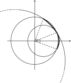
Figure 4. Parameterization of $1/k$ of $\partial E$ (bold line) for $k=4$. Here $B_{1}=B(C_{1},\frac{1}{h_{1}})$ and $B_{2}=B(C_{2},\frac{1}{h_{2}})$

Before proceeding with the proof of Theorem 6.1, we prove a lemma on the uniqueness of the optimal center for a strictly convex set, valid in any dimension $n$. We recall that $x\in{\mathbb{R}}^{n}$ is an optimal center for $E\in{\mathcal{S}}^{n}$ if $|B_{E}|{\alpha}(E)=|E\bigtriangleup(x+B_{E})|$, and that the set of all optimal centers for $E$ is denoted by ${\mathcal{Z}}(E)$.

Lemma 6.4.

Let $E$ be a strictly convex set in ${\mathbb{R}}^{n}$. Then the optimal center of $E$ is unique.

Proof.

Without loss of generality, we assume $B_{E}=B$. Arguing by contradiction, let $x_{1},\ x_{2}\in{\mathcal{Z}}(E)$ with $x_{1}\not=x_{2}$. By the very definition of Fraenkel asymmetry we have that, for $i\in\{1,2\}$,

$$|E\cap(x_{i}+B)|=|B|\left(1-\frac{{\alpha}(E)}{2}\right).$$ (49)

We now set, for $\lambda\in[0,1]$, $x_{\lambda}=\lambda x_{1}+(1-\lambda)x_{2}$ and we observe that

$$E\cap(x_{\lambda}+B)\supseteq\lambda\left(E\cap(x_{1}+B)\right)+(1-\lambda)\left(E\cap(x_{2}+B)\right).$$

Since $E\cap(x_{\lambda}+B)$ is a convex set, we can now exploit the Brunn-Minkowski inequality (see for example [6]) together with (49) to get

$$|E\cap(x_{\lambda}+B)|^{\frac{1}{n}} \geq |\lambda\left(E\cap(x_{1}+B)\right)+(1-\lambda)\left(E\cap(x_{2}+B)\right)|^{\frac{1}{n}}$$

$$\geq \lambda|E\cap(x_{1}+B)|^{\frac{1}{n}}+(1-\lambda)|E\cap(x_{2}+B)|^{\frac{1}{n}}$$

$$= |B|^{\frac{1}{n}}\left(1-\frac{{\alpha}(E)}{2}\right)^{\frac{1}{n}}.$$

The previous inequality shows that $|E\cap(x_{\lambda}+B)|\geq|B|(1-\frac{{\alpha}(E)}{2})$. By the definition of Fraenkel asymmetry, the opposite inequality holds true as well. Thus $|E\cap(x_{\lambda}+B)|=|B|(1-\frac{{\alpha}(E)}{2})$. Such an equality turns out to imply the equality in the Brunn-Minkowski inequality, which is equivalent to saying that, up to translation, the sets $E\cap(x_{\lambda}+B)$ are homotetic to $E\cap(x_{1}+B)$ for all $\lambda\in[0,1]$. Since they all have the same measure, they actually coincide up to translation. As a result, we obtain the flatness of $\partial E\cap(x_{\lambda}+B)$ in the direction of the vector $x_{2}-x_{1}$, but this is in contradiction with the strict convexity of $E$. ∎

Proof of Theorem 6.1.

By the Iterative Selection Principle, and assuming by induction that the coefficients $c_{i}=Q^{(i)}(B)$ are finite for all $i=1,\dots,m-1$, we obtain that ${Q^{(m)}}(B)=\lim\limits_{j}E^{(m)}_{j}$, with $E^{(m)}_{j}$ satisfying the thesis of Theorem 5.1.

Then, again by Theorem 5.1 we may suppose that, for $j$ sufficiently large, $H_{\partial E^{(m)}_{j}}(x)>{\frac{1}{2}}$ for $\mathcal{H}^{1}$-a.e. $x\in\partial E^{(m)}_{j}$, hence $E^{(m)}_{j}$ is a strictly convex set in ${\mathbb{R}}^{2}$. Therefore, by Lemma 6.4 we have ${\mathcal{Z}}(E^{(m)}_{j})=\{x_{0}\}$ and, up to a translation, we may assume that $x_{0}=0$. Therefore, $B$ and ${\mathbb{R}}^{2}\setminus B$ are free regions for $E^{(m)}_{j}$ in the sense of Remark 3.6. By Theorem 5.1 and Remark 3.6 we finally deduce that $E^{(m)}_{j}$ belongs to ${\mathcal{P}}(k)$ for some $k\geq 2$.

Now, by exploiting the annular symmetrization, we will show that necessarily $E^{(m)}_{j}$ is an oval, that is, $E^{(m)}_{j}\in{\mathcal{P}}(2)$. Indeed, assume by contradiction that $E^{(m)}_{j}\in{\mathcal{P}}(k)$ for some $k>2$. In order to simplify notation, we drop some indices and let $E=E^{(m)}_{j}$ be such that $\partial E$ is described by $\gamma_{k}$ given in (48). Then, we will prove that the annular symmetrized set $E^{as}$ with respect to the origin of the reference system satisfies

$$|E^{as}|=|E|,\quad{\alpha}(E^{as})={\alpha}(E),\quad P(E^{as})<P(E),$$

which would give the desired contradiction with the minimality of $E$. To this aim, let $\rho_{1},\rho_{2}>0$ be such that $B(0,\rho_{1})\subset E\subset B(0,\rho_{2})$ and that both $\partial B(0,\rho_{1})$ and $\partial B(0,\rho_{2})$ are tangent to $\partial E$. In other words, the annulus $C_{\rho_{1},\rho_{2}}=B(0,\rho_{2})\setminus B(0,\rho_{1})$ is the one of minimal thickness among those containing $\partial E$. Let us set $S$ as the circular sector which is given in polar coordinates $(r,\theta)$ by $S=[0,+\infty)\times[0,\frac{\pi}{k}]$. Given now $\rho\in(\rho_{1},\rho_{2})$ we set $A_{k}(\rho)$ to be the unique point of intersection of $\partial E$ with $\partial B(0,\rho)$ within the sector $S$, namely $\{A_{k}(\rho)\}=\partial E\cap\partial B(0,\rho)\cap S$. We now introduce the angle $\theta_{k}(\rho)\in[0,\frac{2\pi}{k}]$ such that, in polar coordinates, we can represent $A_{k}(\rho)=(\rho\cos\theta_{k}(\rho),\rho\sin\theta_{k}(\rho))$ and

$$\partial E\cap S=\bigcup_{\rho\in[\rho_{1},\rho_{2}]}A_{k}(\rho)$$

We now have

$${\mathcal{H}}^{1}(E\cap\partial B(0,\rho))=2k\rho\gamma_{k}(\rho).$$ (50)

By definition of the set $E^{as}$ we have that, for all $\rho\in[\rho_{1},\rho_{2}]$

$${\mathcal{H}}^{1}(E\cap\partial B(0,\rho))={\mathcal{H}}^{1}(E^{as}\cap\partial B(0,\rho))$$

and moreover that

$$|E^{as}\cap B|=|E\cap B|,\quad|E^{as}\cap({\mathbb{R}}^{2}\setminus B)|=|E\cap({\mathbb{R}}^{2}\setminus B)|.$$ (51)

By exploiting the same polar parameterization as before, we may write

$$\partial E^{as}=\bigcup_{\rho\in[\rho_{1},\rho_{2}]}A_{2}(\rho)$$

where $A_{2}(\rho)=(\rho\cos\theta_{2}(\rho),\rho\sin\theta_{2}(\rho))$ for $\rho\in[\rho_{1},\rho_{2}]$ and $\theta_{2}(\rho)$ is such that

$${\mathcal{H}}^{1}(E^{as}\cap\partial B(0,\rho))=4\rho\gamma_{2}(\rho).$$ (52)

Comparing (50) and (52) we obtain

$$\theta_{2}(\rho)={\frac{k}{2}}\theta_{k}(\rho)$$ (53)

We finally have

$$P(E^{as}) = 4\int_{\rho_{1}}^{\rho_{2}}\sqrt{1+\rho^{2}(\theta^{\prime}_{2})^{2}}\ d\rho=4\int_{\rho_{1}}^{\rho_{2}}\sqrt{1+\frac{k^{2}}{4}\rho^{2}(\theta^{\prime}_{k})^{2}}\ d\rho$$ (54)

$$< 2k\int_{\rho_{1}}^{\rho_{2}}\sqrt{1+\rho^{2}(\theta^{\prime}_{k})^{2}}\ d\rho=P(E),$$

where the last inequality follows since $k\geq 3$. To conclude the proof we show that the annular symmetrization preserves the strict convexity of our sets, i.e., that for ${\mathcal{H}}$-a.e.$x\in\partial E^{as}$ it holds

$$H_{\partial E^{as}}(x)>0.$$ (55)

In fact, were this the case, and arguing as in Step $1$, we would immediately get ${\mathcal{Z}}(E^{as})=\{x_{0}\}$. Then, by the symmetry of $E^{as}$, $x_{0}=0$ and finally, thanks to (51), we may conclude that ${\alpha}(E^{as})={\alpha}(E)$.

To prove (55) we observe that in $B$ and ${\mathbb{R}}^{2}\setminus\overline{B}$ we have that $H_{\partial E}$ can be computed through the parameterization $\theta_{k}=\theta_{k}(\rho)$ (with a slight abuse of notation, we understand $H_{\partial E}$ as a function of $\rho$) described before. More precisely, the well-known formula

$$0<H_{\partial E}(\rho)=-\frac{\rho^{2}(\theta_{k}^{\prime})^{3}+\rho\theta_{k}^{\prime\prime}+2\theta_{k}^{\prime}}{(1+(\rho\theta_{k}^{\prime})^{2})^{\frac{3}{2}}}$$

holds, and this turns out to imply that $\rho^{2}(\theta_{k}^{\prime})^{3}+\rho\theta_{k}^{\prime\prime}+2\theta_{k}^{\prime}<0$. This last inequality, together with (53) and the fact that, by construction, $\theta^{\prime}_{k}(\rho)<0$, gives

$$H_{\partial E^{as}}(\rho)=-\frac{k}{2}\cdot\frac{\frac{k^{2}}{4}\rho^{2}(\theta_{2}^{\prime})^{3}+\rho\theta_{2}^{\prime\prime}+2\theta_{2}^{\prime}}{(1+(\frac{k}{2}\rho\theta_{2}^{\prime})^{2})^{\frac{3}{2}}}\geq-\frac{k}{2}\cdot\frac{\rho^{2}(\theta_{k}^{\prime})^{3}+\rho\theta_{k}^{\prime\prime}+2\theta_{k}^{\prime}}{(1+(\frac{k}{2}\rho\theta_{2}^{\prime})^{2})^{\frac{3}{2}}}>0.$$

Thanks to (54) and by the definition of ${Q^{(m)}_{j}}$ in (35), we obtain that

$${Q^{(m)}_{j}}(E)>{Q^{(m)}_{j}}(E^{as}),$$ (56)

which is a contradiction with the minimality of $E=E^{(m)}_{j}$. This concludes the proof of the theorem. ∎

Acknowledgements

The research of the first author was partially supported by the European Research Council under FP7, Advanced Grant n. 226234 “Analytic Techniques for Geometric and Functional Inequalities” and by the Deutsche Forschungsgemeinschaft through the Sonderforschungsbereich 611. The second author thanks the Dipartimento di Matematica e Applicazioni “R. Caccioppoli” of the Università degli Studi di Napoli “Federico II”, where he was visiting scholar during the year 2009.

References

• [1] F. J. Almgren, Jr., Existence and regularity almost everywhere of solutions to elliptic variational problems with constraints, Mem. Amer. Math. Soc., 4 (1976), pp. viii+199.
• [2] A. Alvino, V. Ferone, and C. Nitsch, A sharp isoperimetric inequality in the plane, J. Eur. Math. Soc. (JEMS), 13 (2011), pp. 185–206.
• [3] L. Ambrosio, Corso introduttivo alla teoria geometrica della misura ed alle superfici minime, Appunti dei Corsi Tenuti da Docenti della Scuola. [Notes of Courses Given by Teachers at the School], Scuola Normale Superiore, Pisa, 1997.
• [4] L. Ambrosio, N. Fusco, and D. Pallara, Functions of bounded variation and free discontinuity problems, Oxford Mathematical Monographs, The Clarendon Press Oxford University Press, New York, 2000.
• [5] T. Bonnesen, Les Problèmes des isopérimètres et des isépiphanes, Gautier-Villars, Paris, 1929.
• [6] Y. D. Burago and V. A. Zalgaller, Geometric inequalities, vol. 285 of Grundlehren der Mathematischen Wissenschaften [Fundamental Principles of Mathematical Sciences], Springer-Verlag, Berlin, 1988. Translated from the Russian by A. B. Sosinskiĭ, Springer Series in Soviet Mathematics.
• [7] S. Campi, Isoperimetric deficit and convex plane sets of maximum translative discrepancy, Geom. Dedicata, 43 (1992), pp. 71–81.
• [8] A. Cianchi, N. Fusco, F. Maggi, and A. Pratelli, The sharp Sobolev inequality in quantitative form, J. Eur. Math. Soc. (JEMS), 11 (2009), pp. 1105–1139.
• [9]  , On the isoperimetric deficit in the gauss space, Amer. J. Math., (to appear).
• [10] M. Cicalese and G. P. Leonardi, On the absolute minimizers of the quantitative isoperimetric quotient in the plane, forthcoming.
• [11]  , A selection principle for the sharp quantitative isoperimetric inequality, preprint, (2010).
• [12] E. De Giorgi, Frontiere orientate di misura minima, Seminario di Matematica della Scuola Normale Superiore di Pisa, 1960-61, Editrice Tecnico Scientifica, Pisa, 1961.
• [13] A. Figalli, F. Maggi, and A. Pratelli, A mass transportation approach to quantitative isoperimetric inequalities, Invent. Math., 182 (2010), pp. 167–211.
• [14] N. Fusco, F. Maggi, and A. Pratelli, The sharp quantitative Sobolev inequality for functions of bounded variation, J. Funct. Anal., 244 (2007), pp. 315–341.
• [15]  , The sharp quantitative isoperimetric inequality, Ann. of Math. (2), 168 (2008), pp. 941–980.
• [16]  , Stability estimates for certain Faber-Krahn, isocapacitary and Cheeger inequalities, Ann. Sc. Norm. Super. Pisa Cl. Sci. (5), 8 (2009), pp. 51–71.
• [17]  , On the isoperimetric problem with respect to a mixed Euclidean-Gaussian density, preprint, 2010.
• [18] N. Fusco, V. Millot, and M. Morini, A quantitative isoperimetric inequality for fractional perimeters, preprint, 2010.
• [19] E. Giusti, Minimal surfaces and functions of bounded variation, vol. 80 of Monographs in Mathematics, Birkhäuser Verlag, Basel, 1984.
• [20] R. R. Hall, A quantitative isoperimetric inequality in $n$-dimensional space, J. Reine Angew. Math., 428 (1992), pp. 161–176.
• [21] R. R. Hall and W. K. Hayman, A problem in the theory of subordination, J. Anal. Math., 60 (1993), pp. 99–111.
• [22] R. R. Hall, W. K. Hayman, and A. W. Weitsman, On asymmetry and capacity, J. Anal. Math., 56 (1991), pp. 87–123.
• [23] F. Maggi, Some methods for studying stability in isoperimetric type problems, Bull. Amer. Math. Soc. (N.S.), 45 (2008), pp. 367–408.
• [24] U. Massari, Esistenza e regolarità delle ipersuperfici di curvatura media assegnata in $R^{n}$, Arch. Rational Mech. Anal., 55 (1974), pp. 357–382.
• [25] I. Tamanini, Boundaries of Caccioppoli sets with Hölder-continuous normal vector, J. Reine Angew. Math., 334 (1982), pp. 27–39.
• [26]  , Regularity results for almost minimal oriented hypersurfaces in ${R}^{n}$, Quaderni del Dipartimento di Matematica dell’ Università di Lecce, 1 (1984), pp. 1–92.