Amplified optomechanics in a unidirectional ring cavity

Abstract

We investigate optomechanical forces on a nearly lossless scatterer, such as an atom pumped far off-resonance or a micromirror, inside an optical ring cavity. Our model introduces two additional features to the cavity: an isolator is used to prevent circulation and resonant enhancement of the pump laser field and thus to avoid saturation of or damage to the scatterer, and an optical amplifier is used to enhance the effective $Q$-factor of the counterpropagating mode and thus to increase the velocity-dependent forces by amplifying the back-scattered light. We calculate friction forces, momentum diffusion, and steady-state temperatures to demonstrate the advantages of the proposed setup.

1 Introduction and Motivation

Free-space laser cooling [1] has proven to be remarkably successful in cooling simple atomic systems, especially alkali atoms [2]. Relying on the availability of a (quasi-)closed two-level [3] or multi-level [4, 5] system, however, only occasional successes were had with more complicated systems, such as molecules [6, 7]. An alternative to such schemes is cavity–mediated cooling [8, 9, 10, 11], where the interaction of a polarisable particle with a cavity field leads to a Sisyphus–type mechanism [12] that can cool the motion of the particle; no specific energy level scheme is required for this mechanism to operate. Much of this work has been focused on standing-wave (Fabry–Pérot) cavities, where high $Q$-factors can be achieved experimentally to significantly enhance optomechanical forces. However, in the limit of strong scatterers, friction forces in standing-wave cavities become increasingly position-dependent [13], which limits the overall, averaged cooling efficiency. This can be overcome by using ring cavities [14, 15, 16, 17, 18, 19, 20, 21] where the translational symmetry guarantees position-independent forces. On the other hand, ring cavities are usually much larger and of lower $Q$-factor than their standing-wave counterparts. Using a gain medium inside a ring cavity has been proposed [22, 23] to offset these losses, allowing one to effectively ‘convert’ a low-$Q$ cavity into a high-$Q$ one, and thus to increase the effective optomechanical interaction by orders of magnitude. This same concept has also been raised in connection with using optical parametric amplifiers in standard optomechanical systems [24]. Research is also being conducted into using nonlinear media inside cavities [25] as a tool to control the dynamics of a micromechanical oscillator. Another application of ring cavities is in the investigation of collective atomic recoil lasing (CARL) [26], which exploits the spontaneous self-organisation of an atomic ensemble within a ring cavity, induced by a strong pump beam, to amplify a probe beam through Doppler-shifted reflection of the pump. The gain medium is in this case the atomic ensemble itself.

Here, we investigate a different system that shares several features with the above mechanisms. In particular, we consider a particle inside a ring cavity that includes a gain medium, spatially separated from the particle. An isolator is also included in the ring cavity, in such a way as to prevent the pump beam from circulating in the cavity and being amplified; this ensures that the intensity of the field surrounding the particle is always low and thereby circumvents any problems caused by atomic saturation or mirror burning. The Doppler-shifted reflection of the pump from the particle is, on the other hand, allowed to circulate, and its amplification in turn enhances the velocity-dependent forces acting on the particle.

In such a situation, one is able to take advantage of properties inherent to the ring cavity system, such as the fact that the forces acting on the particle do not exhibit any sub-wavelength spatial modulation; this is due to the translational symmetry present in the system [14]. Moreover, modest amplification allows one to use optical fibres to form the ring cavity, opening the door towards increasing the optical length of such cavities. The optomechanical force is, as we will see and in the parameter domain of interest, linearly dependent on the cavity length; lengthening the cavity thus provides further enhancement of the interaction.

This paper is structured as follows. We shall first introduce the physical model, which we proceed to solve using the transfer matrix method (TMM) [27] to obtain the friction force and momentum diffusion acting on the particle. In the good-cavity limit, Section 2.1, simple expressions for these quantities can be obtained, yielding further insight into the system and allowing us to draw some parallels with traditional cavity cooling. In this limit, our model becomes equivalent to one based on a standard master equation approach [14] as outlined in Section 2.2. Realistic numerical values for the various parameters are then used in Section 3 to explore the efficiency and limits of the cooling mechanism. Finally, we will conclude by mentioning some possible extensions to the scheme.

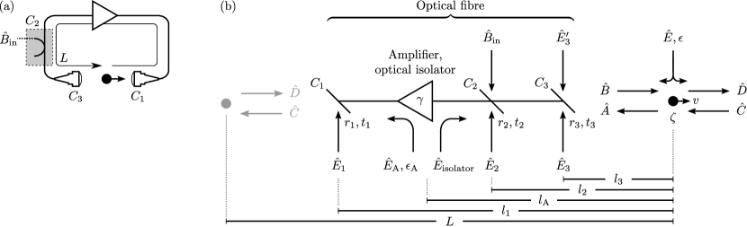
Figure 1: (a) Physical schematic of a polarisable particle in a unidirectional ring cavity, showing the input field $\hat{B}_{\text{in}}$. (b) Equivalent ‘transfer matrix’–style (unfolded) model; the particle is drawn on both sides of this schematic to illustrate the recursive nature of the cavity. The various components are defined in Section 2.

2 General expressions and equilibrium behaviour

The mathematical model of the ring cavity system, schematically drawn in Fig. 1(a), is shown in Fig. 1(b). A particle, characterised by its polarisability $\zeta$, is in a ring cavity of round-trip length $L$. $C_{1,3}$ are the couplers, between which the particle lies, that terminate the fibre-based cavity, and $C_{2}$ is the input coupler that injects a pump beam with wavenumber $k_{0}$ into one of the travelling modes of the cavity. The couplers $C_{i}$ ($i=1,2,3$) have (amplitude) reflection and transmission coefficients $r_{i}$ and $t_{i}=r_{i}+1$, respectively, and are associated with corresponding noise modes $\hat{E}_{i}$. Similarly, the particle itself couples a noise mode $\hat{E}$ into the system with an amplitude $\epsilon$ depending on $\zeta$. The length scales $l_{1}>l_{\text{A}}>l_{2}>l_{3}>0$ are introduced for clarity, but their values are not important for the results of this paper. The cavity contains an optical isolator which prevents the pumped mode from circulating inside the cavity. This avoids resonant enhancement of the pumped mode in the cavity and thus avoids saturating the particle. The backscattered counterpropagating mode, on the other hand, is amplified on every round trip by means of an optical amplifier with gain $\gamma\geq 1$. The amplifier also introduces a noise mode $\hat{E}_{\text{A}}$ with an amplitude $\epsilon_{\text{A}}$ which depends on $\gamma$. The TMM [27] is used to self-consistently solve for the two counterpropagating field amplitudes at every point in the cavity in the presence of the pump field and the noise modes. Note that in the limit where the amplifier is compensating for the ring cavity losses, the amplifier noise is also comparable to the loss-induced noise and must therefore be taken into account in our model.

Using the notation in Fig. 1(a) we can relate the expectation values of the amplitudes of the two input and two scattered field modes interacting with the particle in a one-dimensional scheme, $A(k)=\langle\hat{A}(k)\rangle$, $B(k)=\langle\hat{B}(k)\rangle$, $C(k)=\langle\hat{C}(k)\rangle$, and $D(k)=\langle\hat{D}(k)\rangle$, to $B_{\text{in}}(k)=\langle\hat{B}_{\text{in}}(k)\rangle$ by means of the relations

$$B=r_{2}t_{3}e^{ik_{0}l_{2}}B_{\text{in}}\,,\ C=\alpha A\,,\ \text{and}\ \begin{pmatrix}A\\ B\end{pmatrix}=\hat{M}\begin{pmatrix}C\\ D\end{pmatrix}\,,$$ (1)

where $\alpha(k)=t_{1}t_{2}t_{3}\gamma\exp(ikL)$ is the factor multiplied to the field amplitude every round trip. In the preceding equations, as well as in the following, we do not write the index $k$ for simplicity of presentation. The operators $\hat{A}(k)$, etc., denote the annihilation operators of the various field modes. The three equations Eqs. (1) have a readily apparent physical significance—respectively, they correspond to: the propagation of $\hat{B}_{\text{in}}$ to reach the particle; the feeding back of $\hat{A}$ to $\hat{C}$ through the ring cavity; and the usual transfer matrix relation for a particle interacting with the four fields surrounding it. The first two of these relations are substituted into the third, which subsequently simplifies to

$$\begin{pmatrix}A\\ B_{\text{in}}\end{pmatrix}=\Biggl{(}\begin{bmatrix}1&0\\ 0&r_{2}t_{3}e^{ik_{0}l_{2}}\end{bmatrix}-\hat{M}\begin{bmatrix}\alpha&0\\ 0&0\end{bmatrix}\Biggr{)}^{-1}\hat{M}\begin{pmatrix}0\\ D\end{pmatrix}$$ (2)

If we assume far off-resonant operation, i.e., $\partial\zeta/\partial k=0$, the velocity-dependent transfer matrix $\hat{M}$ can be written as [27, 28]

$$\begin{bmatrix}1+i\zeta&i\zeta-2i\zeta\tfrac{v}{c}+2ik_{0}\zeta\tfrac{v}{c}\partial_{k}\\ -i\zeta-2i\zeta\tfrac{v}{c}+2ik_{0}\zeta\tfrac{v}{c}\partial_{k}&1-i\zeta\end{bmatrix}\,.$$ (3)

The notation $\partial_{k}\equiv\tfrac{\partial}{\partial k}$ is used throughout; note that this partial derivative acts not only on $\alpha(k)$ but also on the field mode amplitudes it precedes. Eq. (2) can be inverted in closed form to first order in $v/c$, similarly to Ref. [28], and can thus be used to find $\mathcal{A}=\sqrt{2\epsilon_{0}S/(\hbar k_{0})}\int A(k)~{}\text{d}k$, $\mathcal{B}=\sqrt{2\epsilon_{0}S/(\hbar k_{0})}\int B(k)~{}\text{d}k$, $\mathcal{C}=\sqrt{2\epsilon_{0}S/(\hbar k_{0})}\int C(k)~{}\text{d}k$, and $\mathcal{D}=\sqrt{2\epsilon_{0}S/(\hbar k_{0})}\int D(k)~{}\text{d}k$, where the normalisation is with respect to the pump beam mode area $S$ and where a monochromatic pump is assumed: $B_{\text{in}}(k)=B_{0}\delta(k-k_{0})$. Here, $\lvert\mathcal{A}\rvert^{2}$, $\lvert\mathcal{B}\rvert^{2}$, etc., are the photon currents in units of photons per second. The expectation value of the force acting on the particle is then given by [27]:

$$\boldsymbol{F}_{\text{full}}=\hbar k_{0}\bigl{(}\lvert\mathcal{A}\rvert^{2}+\lvert\mathcal{B}\rvert^{2}-\lvert\mathcal{C}\rvert^{2}-\lvert\mathcal{D}\rvert^{2}\bigr{)}\,.$$ (4)

The values of $\mathcal{A}$, $\mathcal{B}$, etc., from the solution of Eq. (2) are then substituted into Eq. (4), which we evaluate to first order in $v/c$, in terms of $B_{0}$. After some algebra, we obtain the first main result of this paper—the friction force acting on the particle:

$$\boldsymbol{F}=-8\hbar k_{0}^{2}\tfrac{v}{c}\,\text{Re}\!\left\{\frac{\bigl{(}1-\alpha^{\ast}\bigr{)}\zeta\,\text{Re}\!\left\{\zeta\right\}+i\alpha^{\ast}\zeta\lvert\zeta\rvert^{2}}{1-\alpha-i\zeta}\frac{\partial\alpha}{\partial k}\right\}\frac{\bigl{|}r_{2}t_{3}B_{0}\bigr{|}^{2}}{\bigl{|}1-\alpha-i\zeta\bigr{|}^{2}}\,.$$ (5)

By extending the TMM appropriately, one can keep track of the various noise modes interacting with the system. Eqs. (1) then become

$$\hat{A}=\frac{i\zeta}{1-i\zeta}\hat{B}+\frac{1}{1-i\zeta}\hat{C}+\epsilon\hat{E}\,,$$ (6a)

$$\hat{B}=r_{2}t_{3}e^{ik_{0}l_{2}}\hat{B}_{\text{in}}+t_{2}t_{3}e^{ik_{0}l_{\text{A}}}\hat{E}_{\text{isolator}}+r_{3}e^{ik_{0}l_{3}}\hat{E}_{3}^{\prime}\,,\$$ (6b)

$$\hat{C}=\alpha\hat{A}+r_{1}e^{ik_{0}(L-l_{1})}\hat{E}_{1}+t_{1}r_{2}\gamma e^{ik_{0}(L-l_{2})}\hat{E}_{2}+t_{1}t_{2}r_{3}\gamma e^{ik_{0}(L-l_{3})}\hat{E}_{3}+t_{1}\epsilon_{\text{A}}e^{ik_{0}(L-l_{\text{A}})}\hat{E}_{\text{A}}\,,\text{ and}$$ (6c)

$$\hat{D}=\frac{1}{1-i\zeta}\hat{B}+\frac{i\zeta}{1-i\zeta}\hat{C}+\epsilon\hat{E}\,,$$ (6d)

with $\epsilon=\sqrt{1-\bigl{(}1+\lvert\zeta\rvert\bigr{)}/\lvert 1-i\zeta\rvert^{2}}$ [27] and $\epsilon_{\text{A}}=\sqrt{1-1/\lvert\gamma\rvert^{2}}$ [29]. These equations can be solved simultaneously for $\hat{A}$, $\hat{B}$, $\hat{C}$, and $\hat{D}$, and the solution used to evaluate the momentum diffusion constant, $\boldsymbol{D}$, defined as the two-time autocorrelation function of the force operator, to obtain

$$\boldsymbol{D}\,\delta(t-t^{\prime})=2\epsilon_{0}S\,\hbar k_{0}\Bigl{(} \bigl{[}\hat{A}(t),\hat{A}^{\dagger}(t^{\prime})\bigr{]}\lvert\mathcal{A}\rvert^{2}+\bigl{[}\hat{B}(t),\hat{B}^{\dagger}(t^{\prime})\bigr{]}\lvert\mathcal{B}\rvert^{2}$$

$$+\bigl{[}\hat{C}(t),\hat{C}^{\dagger}(t^{\prime})\bigr{]}\lvert\mathcal{C}\rvert^{2}+\bigl{[}\hat{D}(t),\hat{D}^{\dagger}(t^{\prime})\bigr{]}\lvert\mathcal{D}\rvert^{2}$$

$$+2\,\mathrm{Re}\Bigl{\{}\bigl{[}\hat{A}(t),\hat{B}^{\dagger}(t^{\prime})\bigr{]}\mathcal{A}^{\ast}\mathcal{B}-\bigl{[}\hat{A}(t),\hat{C}^{\dagger}(t^{\prime})\bigr{]}\mathcal{A}^{\ast}\mathcal{C}-\bigl{[}\hat{A}(t),\hat{D}^{\dagger}(t^{\prime})\bigr{]}\mathcal{A}^{\ast}\mathcal{D}$$

$$\qquad\qquad-\bigl{[}\hat{B}(t),\hat{C}^{\dagger}(t^{\prime})\bigr{]}\mathcal{B}^{\ast}\mathcal{C}-\bigl{[}\hat{B}(t),\hat{D}^{\dagger}(t^{\prime})\bigr{]}\mathcal{B}^{\ast}\mathcal{D}$$

$$\qquad\qquad+\bigl{[}\hat{C}(t),\hat{D}^{\dagger}(t^{\prime})\bigr{]}\mathcal{C}^{\ast}\mathcal{D}\Bigr{\}}\Bigr{)}\,,$$ (7)

keeping in mind that most of the noise modes, as well as $\hat{B}_{\text{in}}$, obey the commutation relation $\bigl{[}\hat{E}(t),\hat{E}^{\dagger}(t^{\prime})\bigr{]}=\hbar k_{0}/(2\epsilon_{0}S)\,\delta(t-t^{\prime})$. The sole exception is the noise introduced by the amplifier, $\hat{E}_{\text{A}}$, for which $\bigl{[}\hat{E}_{\text{A}}(t),\hat{E}_{\text{A}}^{\dagger}(t^{\prime})\bigr{]}=-\hbar k_{0}/(2\epsilon_{0}S)\,\delta(t-t^{\prime})$; this is due to the model of the amplifier as a negative temperature heat-bath, whereby the creation and annihilation operators effectively switch rôles. Further discussion of this model can be found in Ref. [29, §7.2]. All the noise modes are independent from one another and from $\hat{B}_{\text{in}}$, which simplifies the expressions considerably.

Finally, the fluctuation–dissipation theorem [3] can be used in conjunction with Eqs. (5) and (2) to estimate the equilibrium temperature that the motion of the particle will tend to:

$$k_{\text{B}}T_{\text{A}}=\frac{\boldsymbol{D}}{-\boldsymbol{F}/v}\,,$$ (8)

where $k_{\text{B}}$ is the Boltzmann constant.

2.1 The good-cavity limit as a simplified case

Before discussing the result of Eqs. (5) and (2), cf. Section 3, we shall make several approximations to obtain a transparent set of equations to briefly explore the equilibrium behaviour of the particle and to compare with a standard master equation approach. In particular, $\zeta$ is assumed to be real, which is tantamount to assuming that the particle suffers no optical absorption, i.e., if it is an atom, that it is pumped far off-resonance. Moreover, the cavity is assumed to be very good ($\lvert t_{1,2,3}\rvert\to 1$) and thus no gain medium is introduced in the cavity ($\gamma=1$). With these simplifications, Eq. (5) reduces to

$$\boldsymbol{F} \approx-8\hbar k_{0}^{2}\tfrac{v}{c}\frac{\zeta^{2}}{\lvert 1-\alpha\rvert^{4}}\,\text{Re}\!\left\{\bigl{(}1-\alpha^{\ast}\bigr{)}^{2}\frac{\partial\alpha}{\partial k}\right\}\bigl{|}r_{2}B_{0}\bigr{|}^{2}$$

$$\approx 16\hbar k_{0}^{2}\zeta^{2}v\frac{\kappa\Delta_{\text{C}}}{\bigl{(}\Delta_{\text{C}}^{2}+\kappa^{2}\bigr{)}^{2}}\frac{1}{\tau}\bigl{|}r_{2}B_{0}\bigr{|}^{2}\,.$$ (9)

In the preceding equations, $\Delta_{\text{C}}$ is the detuning of the pump from cavity resonance, $\kappa$ is the HWHM cavity linewidth,

$$\kappa=\frac{1}{\tau}\frac{1-\lvert t_{1}t_{2}t_{3}\rvert\gamma}{\sqrt{\lvert t_{1}t_{2}t_{3}\rvert\gamma}}\,,$$ (10)

and $\tau=L/c$ is the round-trip time. Using the same approximations as for Eq. (2.1), we also obtain the diffusion constant

$$\boldsymbol{D}\approx 8\hbar^{2}k_{0}^{2}\zeta^{2}\frac{\kappa}{\Delta_{\text{C}}^{2}+\kappa^{2}}\frac{1}{\tau}\bigl{|}r_{2}B_{0}\bigr{|}^{2}\,.$$ (11)

Note that $\gamma=1$ here and therefore $\hat{E}_{\text{A}}$ does not contribute to the diffusion constant. Eqs. (2.1) and (11) hold for the case where $\Delta_{\text{C}}/\kappa$ is not too large. The cavity can be fully described by means of $\kappa$ and the finesse $\mathcal{F}=\pi c/(2L\kappa)$. Let us now set $\Delta_{\text{C}}=-\kappa$ in Eqs. (2.1) and (11), whereby

$$\boldsymbol{F}=-\tfrac{8}{\pi}\hbar k_{0}^{2}\zeta^{2}v\frac{\mathcal{F}}{\kappa}\bigl{|}r_{2}B_{0}\bigr{|}^{2}\,,\text{ and }\boldsymbol{D}=\tfrac{8}{\pi}\hbar^{2}k_{0}^{2}\zeta^{2}\mathcal{F}\bigl{|}r_{2}B_{0}\bigr{|}^{2}\,.$$ (12)

These two expressions have a readily-apparent physical significance; at a constant finesse, decreasing the cavity linewidth by making the cavity longer is equivalent to increasing the retardation effects that underlie this cooling mechanism [30], leading to a stronger friction force. At the same time, this has no effect on the intracavity field strength and therefore does not affect the diffusion. On the other hand, improving the cavity finesse by reducing losses at the couplers increases the intracavity intensity, thereby increasing both the friction force and the momentum diffusion.

Using Eq. (8) together with Eqs. (2.1) and (11) we obtain, for $\Delta_{\text{C}}<0$,

$$T_{\text{A}}\approx\frac{\hbar}{k_{\text{B}}}\biggl{(}\frac{\lvert\Delta_{\text{C}}\rvert}{\kappa}+\frac{\kappa}{\lvert\Delta_{\text{C}}\rvert}\biggr{)}\frac{\kappa}{2}\geq\frac{\hbar}{k_{\text{B}}}\kappa\,,$$ (13)

with the minimum temperature occurring at $\Delta_{\text{C}}=-\kappa$. One notes that this expression is identical to the corresponding one for standard cavity–mediated cooling [12], and can be interpreted in a similar light as the Doppler temperature, albeit with the energy dissipation process shifted from the decay of the atomic excited state to the decay of the cavity field.

A particular feature to note in all the preceding expressions is that they are not spatial averages over the position of the particle, but they do not depend on this position either. As a result of this, the force, momentum diffusion and equilibrium temperature do not in any way depend on the position of the particle along the cavity field in a 1D model. The issue of sub-wavelength modulation of the friction force is a major limitation of cooling methods based on intracavity standing fields, in particular mirror–mediated cooling [28] and cavity–mediated cooling [13].

2.2 Comparison with a semiclassical model

In the good-cavity limit and without gain our TMM model is equivalent to a standard master equation approach with the Hamiltonian

$$\hat{H}= -\hbar\Delta_{\text{a}}\hat{\sigma}^{+}\hat{\sigma}^{-}-\hbar\Delta_{\text{C}}\hat{a}_{\text{C}}^{\dagger}\hat{a}_{\text{C}}$$

$$+\hbar g\bigl{(}\hat{a}_{\text{C}}^{\dagger}\hat{\sigma}^{-}e^{ik_{0}x}+\hat{\sigma}^{+}\hat{a}_{\text{C}}e^{-ik_{0}x}\bigr{)}+\hbar g\bigl{(}a_{\text{P}}^{\ast}\hat{\sigma}^{-}e^{-ik_{0}x}+\hat{\sigma}^{+}a_{\text{P}}e^{ik_{0}x}\bigr{)}\,,$$ (14)

and the Liouvillian terms

$$\mathcal{L}\hat{\rho}=-\Gamma\bigl{(}\hat{\sigma}^{+}\hat{\sigma}^{-}\hat{\rho}-2\hat{\sigma}^{-}\hat{\rho}\hat{\sigma}^{+}+\hat{\rho}\hat{\sigma}^{+}\hat{\sigma}^{-}\bigr{)}-\kappa\bigl{(}\hat{a}_{\text{C}}^{\dagger}\hat{a}_{\text{C}}\hat{\rho}-2\hat{a}_{\text{C}}\hat{\rho}\hat{a}_{\text{C}}^{\dagger}+\hat{\rho}\hat{a}_{\text{C}}^{\dagger}\hat{a}_{\text{C}}\bigr{)}\,,$$ (15)

as adapted from Ref. [14] and modified for a unidirectional cavity where only the unpumped mode is allowed to circulate. Here, $\hat{\rho}$ is the density matrix of the system, $g$ the atom–field coupling strength, $\hat{a}_{\text{C}}$ the annihilation operator of the cavity field, $\hat{\sigma}^{+}$ the atomic dipole raising operator, $\Delta_{\text{a}}$ the detuning from atomic resonance, $\Gamma$ the atomic upper state HWHM linewidth, and $x$ the coordinate of the atom inside the cavity. The pump field is assumed to be unperturbed by its interaction with the atom, and in the above is replaced by a c-number, $a_{\text{P}}$. Calculating the friction force form this model leads again to Eq. (2.1), thus confirming our TMM results by a more standard technique. The advantage of the TMM approach lies in the simplicity and generality of expressions such as Eq. (4), and the ease with which more optical elements can be introduced into the system. As shown above, Eq. (2), the momentum diffusion coefficient is easily calculated from the TMM.

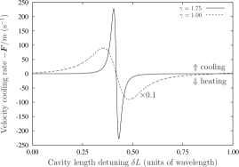
Figure 2: Cooling rate $-(\mathrm{d}v/\mathrm{d}t)/v$ for ⁸⁵Rb pumped $-10\Gamma$ from D₂ resonance inside a ring-cavity with a round-trip length $L=300$ m, for two different values of the amplifier gain $\gamma$. Note that the curve for $\gamma=1$, as drawn, is scaled up by a factor of $10$. The cavity waist is taken to be $10$ $\upmu$m. ($\lvert t_{1}\rvert^{2}=\lvert t_{3}\rvert^{2}=0.5$, $\lvert t_{2}\rvert^{2}=0.99$, $B_{0}$ is chosen such as to give an atomic saturation $s=0.1$.)

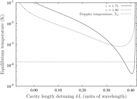
Figure 3: Equilibrium temperature predicted by the transfer matrix model for two values of the amplifier gain $\gamma$. The Doppler temperature for ⁸⁵Rb is also indicated. The horizontal axis differs from that in Fig. 2 mainly because the temperature is only well-defined for regions where the friction force promotes cooling. (Parameters are as in Fig. 2.)

3 Numerical results and discussion

We can use the conversion factor $\lvert B_{0}\rvert^{2}=P/(\hbar k_{0}c)$, where $P$ is the power of the input beam, to evaluate the above equations [notably Eqs. (5) and (2)] numerically in a physically meaningful way. Specifically, the particle is now assumed to be a (two–level) ⁸⁵Rb atom, pumped $-10\Gamma$ from D₂ resonance, where $\Gamma=2\pi\times 3.03$ MHz is the HWHM linewidth of this same transition at a wavelength of ca. $780$ nm; because the detuning is much larger than the linewidth, we simplify the calculations by setting $\partial\zeta/\partial\omega=0$. The beam waist where the particle interacts with the field is taken to be $10$ $\upmu$m. With the parameters in Fig. 2, the power is reduced by a factor of $1/\lvert t_{1}t_{2}t_{3}\rvert^{2}=4.04$ with each round-trip, in the presence of no gain in the amplifier. We shall compare this case to the low-gain case; the gain of the amplifier we consider is constrained to be small enough that $\lvert\alpha\rvert^{2}=\lvert t_{1}t_{2}t_{3}\gamma|^{2}<1$. Under these conditions, there is no exponential build-up of intensity inside the cavity and the system is stable. A cavity with a large enough gain that $\lvert\alpha\rvert^{2}>1$ would effectively be a laser cavity. Such a system would have no stable state in our model, since we assume that the gain medium is not depleted, and will therefore not be considered further in this paper.

Fig. 2 shows the friction force acting on the particle, and Fig. 3 the equilibrium temperature, as the length of the cavity is tuned on the scale of one wavelength. In each of these two figures two cases are shown, one representing no gain in the amplifier ($\gamma=1$) and one representing a low-gain amplifier ($\gamma=1.75$); note that in both cases the condition $\lvert\alpha\rvert^{2}<1$ is satisfied.

In order to provide a fair comparison between these two cases, we choose the pump amplitude $B_{\text{in}}$ such that the saturation of the particle is the same in the two cases. This ensures that any difference in cooling performance is not due to a simple increase in intensity. Since the TMM as presented here is based on a linear model of the particle, our results presented above are only valid in the limit of saturation parameter much smaller than $1$. Thus, as a basis for the numerical comparisons between the two different cases, we choose to set the saturation parameter to $0.1$. Fig. 2 shows that under these conditions the amplified system leads to a significant, approximately $25$-fold, enhancement of the maximum friction force. This can therefore be attributed unambiguously to the effective enhancement of the cavity $Q$-factor by the amplifier.

However, for the parameters considered here, in particular for small particle polarisability $\zeta$ and for $\lvert\alpha\rvert^{2}<1$, the counterpropagating mode intensity is much smaller than that of the pumped mode, even if the former is amplified. Thus, the intracavity field is always dominated by the pump beam, whereas the friction force is mostly dependent on the Doppler-shifted reflection of the pump from the particle. Specifically, for the parameters used above we find that the total field intensity changes by less than 1% when the gain is increased from 1 to 1.75. Hence, similar results to those of Fig. 2 are obtained even without pump normalisation.

The steady-state temperature, obtained by the ratio of diffusion and friction, Eq. (8), is shown in Fig. 3 for the same parameters as above. We observe that the broader resonance in the friction as a function of cavity detuning (i.e., of cavity length), shown in Fig. 2, also leads to a wider range of lower temperatures compared to the amplified case. However, as expected, within the narrower resonance of the amplified system where the friction is significantly enhanced, the stationary temperature is also significantly reduced. We see that while the maximum friction force is increased by a factor of $25.4$, the lowest achievable temperature is decreased by a factor of $19.9$ when switching from $\gamma=1$ to $\gamma=1.75$. While the overall cavity intensity is dominated by the pump field, and is therefore hardly affected by the amplifier, the diffusion is actually dominated by the interaction of the weak counterpropagating field with the pump field. This can be seen most clearly by the strong detuning dependence of the analytic expression for $\boldsymbol{D}$ in the good-cavity limit, Eq. (11). As a consequence, the lowest achievable temperature is improved by a slightly smaller factor than the maximum friction coefficient. This is consistent with the idea that the amplifier not only increases the cavity lifetime, but also adds a small amount of additional noise into the system. Nevertheless, a strong enhancement of the cooling efficiency is observed in the presence of the amplifier.

4 Conclusions and Outlook

We have presented a modified model for optomechanics inside ring cavities where only one of the counter-propagating fields in the cavity is allowed to circulate. By pumping the other mode and using a gain medium inside the cavity, one can greatly improve the optomechanical force acting on a polarisable particle inside the cavity, regardless of its energy level structure, without bringing about ill effects such as saturation or mirror burning. The conceptual introduction of a gain medium inside the cavity brings about several interesting possibilities. We have considered using this gain medium to offset losses inherent in the cavity, thereby improving its $Q$-factor significantly. This renders possible the use of optical fibres to build the cavity. One could also envisage using doped fibre amplifiers [31] to provide a distributed gain medium along the cavity. In this paper, we only considered low-gain media, such that the total losses in the cavity still exceeded the gain. Higher gains could be used to explore and exploit novel phenomena such as optomechanical interactions of weakly reflective micromirrors inside laser cavities and will be the subject of future work.

References

- [1] S. Chu, L. Hollberg, J. E. Bjorkholm, et al., Phys. Rev. Lett. 55 48 (1985).
- [2] S. Chu, Rev. Mod. Phys. 70 685 (1998).
- [3] H. J. Metcalf and P. van der Straten, J. Opt. Soc. Am. B 20 887 (2003).
- [4] J. Dalibard and C. Cohen-Tannoudji, J. Opt. Soc. Am. B 6 2023 (1989).
- [5] P. J. Ungar, D. S. Weiss, E. Riis, et al., J. Opt. Soc. Am. B 6 2058 (1989).
- [6] M. Zeppenfeld, M. Motsch, P. W. H. Pinkse, et al., Phys. Rev. A 80 041401 (2009).
- [7] E. S. Shuman, J. F. Barry and D. DeMille, Nature 467 820 (2010).
- [8] G. Hechenblaikner, M. Gangl, P. Horak, et al., Phys. Rev. A 58 3030 (1998).
- [9] P. Maunz, T. Puppe, I. Schuster, et al., Nature 428 50 (2004).
- [10] D. R. Leibrandt, J. Labaziewicz, V. Vuletić, et al., Phys. Rev. Lett. 103 103001 (2009).
- [11] M. Koch, C. Sames, A. Kubanek, et al., Phys. Rev. Lett. 105 173003 (2010).
- [12] P. Horak, G. Hechenblaikner, K. M. Gheri, et al., Phys. Rev. Lett. 79 4974 (1997).
- [13] A. Xuereb, P. Domokos, P. Horak, et al., submitted to Eur. Phys. J. D (2010).
- [14] M. Gangl and H. Ritsch, Phys. Rev. A 61 043405 (2000).
- [15] T. Elsässer, B. Nagorny and A. Hemmerich, Phys. Rev. A 67 051401 (2003).
- [16] D. Kruse, M. Ruder, J. Benhelm, et al., Phys. Rev. A 67 051802 (2003).
- [17] D. Nagy, J. K. Asbóth and P. Domokos, Acta Phys. Hung. B 26 141 (2006).
- [18] S. Slama, S. Bux, G. Krenz, et al., Phys. Rev. Lett. 98 053603 (2007).
- [19] M. Hemmerling and G. R. M. Robb, Phys. Rev. A 82 053420 (2010).
- [20] R. J. Schulze, C. Genes and H. Ritsch, Phys. Rev. A 81 063820 (2010).
- [21] W. Niedenzu, R. Schulze, A. Vukics, et al., Phys. Rev. A 82 043605 (2010).
- [22] V. Vuletić, Laser Physics at the Limits (Springer, 2001), chap. Cavity Cooling with a Hot Cavity, 67–74.
- [23] T. Salzburger and H. Ritsch, Phys. Rev. A 74 033806 (2006).
- [24] S. Huang and G. S. Agarwal, Phys. Rev. A 79 013821 (2009).
- [25] T. Kumar, A. B. Bhattacherjee and Manmohan, Phys. Rev. A 81 013835 (2010).
- [26] R. Bonifacio, L. De Salvo, L. M. Narducci, et al., Phys. Rev. A 50 1716 (1994).
- [27] A. Xuereb, P. Domokos, J. Asbóth, et al., Phys. Rev. A 79 053810 (2009).
- [28] A. Xuereb, T. Freegarde, P. Horak, et al., Phys. Rev. Lett. 105 013602 (2010).
- [29] C. W. Gardiner and P. Zoller, Quantum Noise (Springer, 2004).
- [30] A. Xuereb, P. Horak and T. Freegarde, Phys. Rev. A 80 013836 (2009).
- [31] P. C. Becker, N. A. Olsson and J. R. Simpson, Erbium-Doped Fiber Amplifiers: Fundamentals and Technology (Optics and Photonics) (Academic Press, 1999).