Exact exchange potential evaluated solely
from occupied Kohn-Sham and Hartree-Fock solutions

Abstract

The reported new algorithm determines the exact exchange potential $v_{\text{x}}$ in a iterative way using energy and orbital shifts (ES, OS) obtained — with finite-difference formulas — from the solutions (occupied orbitals and their energies) of the Hartree-Fock-like equation and the Kohn-Sham-like equation, the former used for the initial approximation to $v_{\text{x}}$ and the latter — for increments of ES and OS due to subsequent changes of $v_{\text{x}}$. Thus, solution of the differential equations for OS, used by Kümmel and Perdew (KP) [Phys. Rev. Lett. 90, 043004 (2003)], is avoided. The iterated exchange potential, expressed in terms of ES and OS, is improved by modifying ES at odd iteration steps and OS at even steps. The modification formulas are related to the OEP equation (satisfied at convergence) written as the condition of vanishing density shift (DS) — they are obtained, respectively, by enforcing its satisfaction through corrections to approximate OS and by determining optimal ES that minimize the DS norm. The proposed method, successfully tested for several closed-(sub)shell atoms, from Be to Kr, within the DFT exchange-only approximation, proves highly efficient. The calculations using pseudospectral method for representing orbitals give iterative sequences of approximate exchange potentials (starting with the Krieger-Li-Iafrate approximation) that rapidly approach the exact $v_{\text{x}}$ so that, for Ne, Ar and Zn, the corresponding DS norm becomes less than $10^{-6}$ after 13, 13 and 9 iteration steps for a given electron density. In self-consistent density calculations, orbital energies of $10^{-4}$ Hartree accuracy are obtained for these atoms after, respectively, 9, 12 and 12 density iteration steps, each involving just 2 steps of $v_{\text{x}}$ iteration, while the accuracy limit of $10^{-6}$–$10^{-7}$ Hartree is reached after 20 density iterations.

I Introduction

Modern ab initio calculations for molecular and condensed matter systems are most frequently based on the density functional theory (DFT), which gives the prescription for determining properties of an interacting $N$-electron system (in its ground state) with the aid of the Kohn-Sham (KS) scheme describing a corresponding system of non-interacting particles PY89 ; DG90 ; SGWKV05 ; PK03 ; HK64 . While the DFT approach simplifies enormously the description of many-electron systems, application of the KS scheme requires the knowledge of the exchange-correlation (xc) potential which is the part of the KS Hamiltonian that represents all complex correlations between electrons in the physical system (due to their fermionic character and Coulomb interactions). The xc potential is defined as the functional derivative $v_{\text{xc}\sigma}({\bm{r}})=\delta E_{\text{x}c}[n_{\uparrow},n_{\downarrow}]/\delta n_{\sigma}({\bm{r}})$ of the xc energy $E_{\text{xc}}$ with respect to the density $n_{\sigma}({\bm{r}})$ of electrons with spin $\sigma\ (=\uparrow,\downarrow)$ but its exact form remains unknown, so it is usually found using the local-density or generalized-gradient approximations (LDA, GGA) to the functional $E_{\text{xc}}[n_{\uparrow},n_{\downarrow}]$. Although this approach has proved to be highly successful in calculations of numerous physical properties, it fails in some cases (e.g., for energies of bound unoccupied states) due to the incomplete cancelation of Coulomb self-interaction in the KS potential including $v_{\text{xc}\sigma}$ obtained with LDA or GGA. Such shortcomings of these approximate xc potentials are largely removed when the exact exchange potential $v_{\text{x}\sigma}({\bm{r}})$, which is the dominant part of $v_{\text{xc}\sigma}=v_{\text{x}\sigma}+v_{\text{c}\sigma}$, is used. It is defined as $v_{\text{x}\sigma}({\bm{r}})=\delta E_{\text{x}}[n_{\sigma}]/\delta n_{\sigma}({\bm{r}})$ with the $\sigma$-subsystem exchange energy $E_{\text{x}}$ given explicitly in terms of the occupied KS orbitals which are obtained with the potential $v_{\text{s}\sigma}$ that corresponds to $n_{\sigma}$ (by virtue of the Hohenberg-Kohn theorem HK64 ). The KS potential $v_{\text{s}\sigma}({\bm{r}})$ including the so defined exact $v_{\text{x}\sigma}$ is free from self-interaction and, consequently, it has the proper asymptotic dependence ($-1/r$ for atoms), unlike $v_{\text{s}\sigma}({\bm{r}})$ obtained with LDA or GGA.

The KS orbitals $\phi_{a\sigma}({\bm{r}})$ and their energies $\epsilon_{a\sigma}$ are eigensolutions of the KS equation

$$\hat{h}_{\text{s}\sigma}({\bm{r}})\,\phi_{a\sigma}({\bm{r}})=\epsilon_{a\sigma}\,\phi_{a\sigma}({\bm{r}})\,,\ \ \epsilon_{a\sigma}<\epsilon_{a+1,\sigma}\,,$$ (1a)

where

$$\hat{h}_{\text{s}\sigma}({\bm{r}})=\hat{t}({\bm{r}})+v_{\text{s}\sigma}({\bm{r}})\,,\ \ \ \hat{t}({\bm{r}})=-{\textstyle\frac{1}{2}}\bm{\nabla}^{2}({\bm{r}})$$ (1b)

(atomic units used throughout the paper, orbitals chosen to be real) while the effective local KS potential $v_{\text{s}\sigma}(\bm{r})$ is the sum of the external, electrostatic and xc terms. This potential is modified, for convenience in theoretical considerations, by adding an infinitesimal symmetry-breaking term to remove any possible degeneracy (cf. Ref. KKGG99, ), and by enclosing the system in a large box to have fully discrete energy spectrum (and to guarantee convergence of spatial integrals). The latter modification of $v_{\text{s}\sigma}$ is not required for bound orbitals and it is not used by us in practical calculations of their wavefunctions and energies with the presently applied numerical method (Sec. VII.1). The spin-up, $n_{\uparrow}({\bf r})$, and spin-down, $n_{\downarrow}({\bf r})$, electron densities are determined with the occupied KS orbitals $\phi_{a\sigma}$ ($a=1,\ldots,N_{\sigma}$, $N_{\uparrow}+N_{\downarrow}=N$) through the relation

$$n_{\sigma}({\bm{r}})=n[\{\phi_{a\sigma}\}]({\bm{r}})\equiv\sum_{a=1}^{N_{\sigma}}\phi_{a\sigma}^{2}({\bm{r}})\,.$$ (2)

Since the exchange potential $v_{\text{x}\sigma}$ depends only on the density $n_{\sigma}$ and it is expressible in terms of $\sigma$-subsystem characteristics, the dependence on the spin index $\sigma$ in $v_{\text{x}\sigma}$, $n_{\sigma}$, $N_{\sigma}$, $\phi_{a\sigma}$ etc. can be suppressed hereafter and all following discussion refers to one of the spin-up or spin-down sub-systems separately.

The exact exchange potential $v_{\text{x}}({\bm{r}})=\delta E_{\text{x}}[n]/\delta n({\bm{r}})$, defined with exact $E_{\text{x}}$, satisfies an integral equation the kernel of which is the static KS linear response function involving all (occupied and unoccupied) KS orbitals of given spin. This equation was originally derived within the optimized-effective-potential (OEP) approach TSh76 ; WPC90 ; KLI92 ; E03 and it can be also obtained GL94 when $v_{\text{x}\sigma}(\bf r)$ is identified as the first-order term in the xc potential expansion resulting from adiabatic switching the electron-electron interaction in the many-electron Hamiltonian GL93 . The OEP equation for $v_{\text{x}}$ can be solved numerically within a spatial grid representation for atoms TSh76 ; KLI92 ; LKI93 ; EV93a ; ED99 ; EHD00 but the involved determination of the KS response function matrix makes this approach inefficient for larger systems. The solution of the OEP equation with a finite basis for orbitals and an auxiliary basis for the response function GL94 ; G99 ; IHB99 is usually very troublesome for atoms and molecules since it requires careful balancing of the two bases to avoid unphysical oscillations of $v_{\text{x}}({\bm{r}})$ HIGBBT01 ; DSG01 ; HGSG07 . Similar problems due to basis imbalance are encountered SSD06 ; HBBY07 ; HBY08 ; GHJL08 when the exact $v_{\text{x}}$, expressed in an auxiliary basis, is found by following directly the OEP approach, i.e., by minimizing the HF-like energy expression for total energy given in terms of occupied (KS) orbitals obtained with a local potential $v_{\text{s}}$; see Ref. YW02, . An alternative method of solving the OEP equation in orbital basis representation, which avoids the use of an auxiliary basis by expressing potentials in terms of the products of occupied and unoccupied KS orbitals, has been proposed very recently FKF10 .

A different approach to determination of the exact $v_{\text{x}}$, introduced by Kümmel and Perdew (KP) KP03 , uses the OEP equation rewritten in terms of the occupied KS orbitals and the corresponding orbital shifts (OS) KLI92 ; GKKG00 ; see Sec. III.1. The latter are solutions of $N$ non-homogeneous linear differential equations, hearafter called the KP equations, which depend on the unknown $v_{\text{x}}$. The so posed problem of determining $v_{\text{x}}$ (for a given density) has so far been solved in two ways (Sec. III.3): (i) by iterating $v_{\text{x}}$ and the OS KP03 , (ii) with our previously developed algorithm CH07 where $v_{\text{x}\sigma}$ is found without any iteration, using the solution of the system of equations (algebraic and differential) obtained by a suitable combination of the OEP and KP equations. A further discussion on the exact exchange potential and its orbital-dependent approximations, methods of their determination and applications can be found in the recent review KK08 by Kümmel and Kronik.

In the present work, we determine the exact exchange potential with a novel iterative method based on the representation of approximate $v_{\text{x}}$ (at each iteration step) in terms of the corresponding OS and energy shifts (ES). Such representation was previously derived in Refs. KLI92, ; GKKG00, ; KP03, for the exact $v_{\text{x}}$, but it is now recognized to be an identity relation holding for any local multiplicative potential (Sec. II), in a similar way as the relations previously found in Ref. HC05, . Our new algorithm, summarized in Sec. VI, consists of (i) calculating the OS and ES with a finite-difference formula from solutions of the KS(-like) and Hartree-Fock(HF)-like equations (Sec. IV), and (ii) iterating $v_{\text{x}}$ (for a given density) by modification of its ES and OS terms with an appropriate use of the OEP equation (Secs. III.4, V), (iii) iterating the KS potential $v_{\text{s}}$ to obtain the convergent density. Thus, solution of the KP equations is avoided, while the iteration of $v_{\text{x}}$ is done in a different way than in Ref. KP03, . The method for calculating of the OS and ES follows a recent finding that the OS are well represented by the differences of the respective occupied KS and HF orbitals, see Table I in Ref. C10, (note that in the latter work HF orbital-specific exchange potentials are shown to map very accurately onto $v_{\text{x}}$ and thus the outstanding proximity between the HF and KS orbitals is explained).

The efficiency of the proposed algorithm is tested (Sec. VII) for several closed-(sub)shell atoms from Be to Kr within the exchange-only KS scheme where the correlation energy $E_{\text{c}}$ is neglected together with the potential $v_{\text{c}}$, a part of the xc potential, thus leaving only $v_{\text{x}}$. In the performed tests, the obtained exchange potentials, which are, in fact, very accurate approximations to the exact $v_{\text{x}}$, are compared with the exact exchange potential (used as a reference) determined with extremely high accuracy using our non-iterative algorithm CH07 . Similar comparison is done between the corresponding electron densities and orbital energies.

II Identity satisfied by any local potential

We find it useful to begin our presentation of a new algorithm for the exact exchange potential $v_{\text{x}}({\bm{r}})\equiv v_{\text{x}}^{\text{E}}({\bm{r}})$ by our reformulation of the investigation of Krieger et al. KLI92 , continued next by Grabo et al. GKKG00 and by Kümmel and Perdew KP03 . It is given in a form of an identity satisfied by an arbitrary local (multiplicative) potential $v_{\text{x}}^{\text{L}}({\bm{r}})$ [some restriction on it will be indicated below Eq. (11c)]. This identity is written in terms of the occupied KS orbitals $\{\phi_{a}({\bm{r}})\}_{a=1}^{N}$, Eq. (1a) [directly and via the density $n({\bm{r}})$, Eq. (2)], auxiliary constants — the energy shifts (ES) $\{D_{aa}^{\text{L}}\}_{a=1}^{N}$ and auxiliary functions — the orbital shifts (OS) $\{\delta\phi_{a}^{\text{L}}({\bm{r}})\}_{a=1}^{N}$, namely

$$v_{\text{x}}^{\text{L}}({\bm{r}}) = v_{\text{x}}^{\text{Sl}}[\{\phi_{a}\}]({\bm{r}})+v_{\text{x}}^{\text{ES}}[\{D_{aa}^{\text{L}}\},\{\phi_{a}\}]({\bm{r}})$$ (3)

$$\mbox{}+v_{\text{x}}^{\text{OS}}[\{\delta\phi_{a}^{\text{L}}\},\{\phi_{a}\}]({\bm{r}})\,,$$

where

$$v_{\text{x}}^{\text{Sl}}[\{\phi_{a}\}]({\bm{r}})=\frac{1}{n({\bm{r}})}\sum_{a=1}^{N}\phi_{a}({\bm{r}})\hat{v}_{\text{x}}^{\text{F}}[\{\phi_{b}\}]({\bm{r}})\phi_{a}({\bm{r}})$$ (4)

is known as the Slater potential, while

$$v_{\text{x}}^{\text{ES}}[\{D_{aa}^{\text{L}}\},\{\phi_{a}\}]({\bm{r}})\equiv v_{\text{x}}^{\text{ESL}}({\bm{r}})=\sum_{a=1}^{N}v_{\text{x}}^{aa}({\bm{r}})D_{aa}^{\text{L}}\,,$$ (5a)

where

$$v_{\text{x}}^{aa}({\bm{r}})=\frac{\phi_{a}^{2}({\bm{r}})}{n({\bm{r}})}\,,$$ (5b)

and

$$v_{\text{x}}^{\text{OS}}[\{\delta\phi_{a}^{\text{L}}\},\{\phi_{a}\}]({\bm{r}})\equiv v_{\text{x}}^{\text{OSL}}({\bm{r}})=\sum_{a=1}^{N}\hat{v}_{\text{x}a}^{\text{OS}}({\bm{r}})\,\delta\phi_{a}^{\text{L}}({\bm{r}})\equiv$$

$$\frac{1}{n({\bm{r}})}\sum_{a=1}^{N}\biglb\{\delta\phi_{a}^{\text{L}}({\bm{r}})\,\hat{t}({\bm{r}})\phi_{a}({\bm{r}})-\phi_{a}({\bm{r}})\,\hat{t}({\bm{r}})\delta\phi_{a}^{\text{L}}({\bm{r}})\bigrb\}\,,$$ (6)

are the ES and OS components of the potential. The OS operator $\hat{v}_{\text{x}a}^{\text{OS}}$ [occurring in Eq. (6)] includes a differential operator $\hat{t}({\bm{r}})$, while the Fock exchange operator $\hat{v}_{\text{x}}^{\text{F}}$ [occurring in Eq. (4)] is a non-local integral one defined by

$$\hat{v}_{\text{x}}^{\text{F}}[\{\phi_{a}\}]({\bm{r}})\,\varphi({\bm{r}})=-\int\text{d}^{3}r^{\prime}\sum_{a=1}^{N}\frac{\phi_{a}({\bm{r}})\,\phi_{a}({\bm{r}}^{\prime})\,\varphi({\bm{r}}^{\prime})}{|{\bm{r}}-{\bm{r}}^{\prime}|}\,.$$ (7)

The ES and OS for the potential $v_{\text{x}}^{\text{L}}$ are given by

$$D_{aa}^{\text{L}} = D_{aa}[v_{\text{x}}^{\text{L}}-\hat{v}_{\text{x}}^{\text{F}}]\,,$$ (8)

$$\delta\phi_{a}^{\text{L}}({\bm{r}}) = \delta\phi_{a}[v_{\text{x}}^{\text{L}}-\hat{v}_{\text{x}}^{\text{F}}]({\bm{r}})\,,$$ (9)

where for any potentials difference $\delta\hat{v}({\bm{r}})$ the ES $D_{aa}[\delta\hat{v}]$ are defined as its matrix elements

$$D_{aa}[\delta\hat{v}]=\langle\phi_{a}|\delta\hat{v}|\phi_{a}\rangle\,,$$ (10)

while the OS $\delta\phi_{a}[\delta\hat{v}]({\bm{r}})$ are solutions of the differential equation involving $\delta\hat{v}({\bm{r}})$

$$\Bigl{[}\hat{t}({\bm{r}})+{v}_{\text{s}}({\bm{r}})-\epsilon_{a}\Bigr{]}\delta\phi_{a}[\delta\hat{v}]({\bm{r}})=-\hat{w}_{a}[\delta\hat{v}]({\bm{r}})\,\phi_{a}({\bm{r}})\,,$$ (11a)

where the right-hand side operator is

$$\hat{w}_{a}[\delta\hat{v}]({\bm{r}})=\delta\hat{v}({\bm{r}})-\langle\phi_{a}|\delta\hat{v}|\phi_{a}\rangle\,.$$ (11b)

These solutions must satisfy the same boundary conditions as orbitals. In addition, they must satisfy the orthogonality requirement

$$\langle\phi_{a}|\delta\phi_{a}[\delta\hat{v}]\rangle=0\,.$$ (11c)

The identity (3) concerns only such potentials $$v_{\text{x}}^{\text{L}} \delta\phi_{a}[v_{\text{x}}^{\text{L}}-\hat{v}_{\text{x}}^{\text{F}}] \langle\phi_{a}|\hat{w}_{a}|\phi_{a}\rangle=0 \hat{w}_{a}[\delta\hat{v}] c$$ that the solution of Eq. (11) exists. Note that , and that is invariant with respect to a constant shift of its argument, therefore

$$\delta\phi_{a}[\delta\hat{v}+c]({\bm{r}})=\delta\phi_{a}[\delta\hat{v}]({\bm{r}})\,.$$ (11d)

As we see, all terms on the right-hand side of the identity (3) can be evaluated knowing only $v_{\text{x}}^{\text{L}}$, the occupied KS solutions $\{\phi_{a},\epsilon_{a}\}_{a=1}^{N}$ and the KS potential ${v}_{\text{s}}$. The dependence on $v_{\text{x}}^{\text{L}}$ enters via the functionals ES and OS, Eqs. (8) and (9). The dependence on ${\bm{r}}$ enters the separate components via $\{\phi_{a}({\bm{r}})\}$, $n({\bm{r}})$, $\hat{v}_{\text{x}}^{\text{F}}({\bm{r}})$ and $\{\delta\phi_{a}^{\text{L}}({\bm{r}})\}$. The identity (3) is similar to other three identities obtained by us in our paper HC05 . Any local potential potential expressed according to the the identity (3) will be named to have the canonical form. This identity will be used by us for $v_{\text{x}}^{\text{L}}$ representing an approximate exchange potential in the process of iterative improvement leading to the exact one.

The validity of Eq. (3) can be proven quite simply. For $\delta\hat{v}=v_{\text{x}}^{\text{L}}-\hat{v}_{\text{x}}^{\text{F}}$ one should multiply both sides of Eq. (11a) by $\phi_{a}({\bm{r}})$, sum up over $a$ from 1 to $N$, use definitions (2) and (1b), and utilize Eq. (1a) to replace $\epsilon_{a}\,\phi_{a}$ by the equivalent expression. Locality of $v_{\text{x}}^{\text{L}}$ and $v_{\text{s}}$ is to be taken into account. It should be noted that the requirement (11c) is not involved in this procedure. However, it defines uniquely the particular solution of Eq. (11a) that allows for expressing $\delta\phi_{a}^{\text{L}}$ in the equivalent perturbation-theory form, Sec. IV. A general solution is $\delta\phi_{a}^{\text{L}}+c_{a}\phi_{a}$, with an arbitrary constant $c_{a}$.

There are interesting properties of the canonical representation of a local potential. The replacement $\delta\phi_{a}^{\text{L}}\rightarrow\delta\phi_{a}^{\text{L}}+c_{a}\phi_{a}$ (with $c_{a}$ — a constant) does not change the OS potential, Eq. (6). While the OS, Eq. (9), are insensitive to the replacement $v_{\text{x}}^{\text{L}}\rightarrow v_{\text{x}}^{\text{L}}+c_{\text{x}}^{\text{L}}$ (with $c_{\text{x}}^{\text{L}}$ — a constant), see Eq. (11d), the ES, Eq. (8), are changed by this replacement

$$D_{aa}^{\text{L}}\rightarrow D_{aa}^{\text{L}}+c_{\text{x}}^{\text{L}}\,.$$ (12)

Therefore, due to the obvious identity [see Eq. (5b)]

$$\forall{\bm{r}}\,,\ \ \sum_{a=1}^{N}v_{\text{x}}^{aa}({\bm{r}})=1\,,$$ (13)

the ES potential, Eq. (5a), transforms as

$$v_{\text{x}}^{\text{ES}}({\bm{r}})\rightarrow v_{\text{x}}^{\text{ES}}({\bm{r}})+c_{\text{x}}^{\text{L}}\,.$$ (14)

Thus, the identity (3) remains valid for the potential $v_{\text{x}}^{\text{L}}$ replaced by $(v_{\text{x}}^{\text{L}}+c_{\text{x}}^{\text{L}})$ on both sides of the identity.

It proves convenient for further applications to fix the additive constant of an approximate exchange potential $v_{\text{x}}^{\text{L}}({\bm{r}})$ by the replacement

$$D_{aa}^{\text{L}}:=D_{aa}^{\text{L}}-D_{NN}^{\text{L}}\,,$$ (15)

resulting in

$$D_{NN}^{\text{L}}=0\,.$$ (16)

With Eq. (16) satisfied, the potential $v_{\text{x}}^{\text{ES}}[\{D_{aa}^{\text{L}}\},\{\phi_{a}\}]({\bm{r}})$ is exponentially small in the large-$r$ region for a general direction ${\bm{r}}/r$ (i.e. for ${\bm{r}}$ not laying on the nodal surface of $\phi_{N}({\bm{r}})$, if this orbital possesses such surface extending to the asymptotic region, see Della Sala and Görling, DSG02 ). The Slater potential $v_{\text{x}}^{\text{Sl}}({\bm{r}})$ is known to behave asymptotically as $-1/r$. Thus, the asymptotic behavior of the OS potential is needed to find the asymptotic form of $v_{\text{x}}^{\text{L}}({\bm{r}})$ from its canonical representation.

For the exact (E) exchange potential, $v_{\text{x}}^{\text{L}}=v_{\text{x}}^{\text{E}}$, its OS part $v_{\text{x}}^{\text{OSE}}({\bm{r}})$, Eq. (6), exponentially vanishes at $r\rightarrow\infty$, so it is asymptotically smaller than $v_{\text{x}}^{\text{Sl}}({\bm{r}})$. This is a consequence of the OEP equation [see Eq. (18a) below] which implies the OS $\delta\phi_{N-1}^{\text{E}}$ and $\delta\phi_{N}^{\text{E}}$ in the large-$r$ region must behave (with accuracy to their leading exponential factors) as $-C_{N}\phi_{N}$ and $C_{N}\phi_{N-1}$, respectively, in order to satisfy $\sum_{a=1}^{N}2\phi_{a}\,\delta\phi_{a}^{\text{E}}=0$. Then $v_{\text{x}}^{\text{OSE}}$ will be dominated by the terms with $a=N-1$ and $a=N$, each as small as $\phi_{N-1}/\phi_{N}$.

However, for an arbitrary local potential $v_{\text{x}}^{\text{L}}$, which does not satisfy the OEP equation, the respective OS potential $v_{\text{x}}^{\text{OSL}}({\bm{r}})$ may be finite at $r\rightarrow\infty$. In this case, imposing the condition (16) — though it results in the asymptotically vanishing term $v_{\text{x}}^{\text{ESL}}$ (for a general direction) — leads to $v_{\text{x}}^{\text{L}}({\bm{r}})$ that tends to a finite value $v_{\text{x}}^{\text{L}}(\infty)=v_{\text{x}}^{\text{OSL}}(\infty)$.

III Exact exchange potential

III.1 Density shift and the OEP equation

Considering the exchange potential to be a functional of the given density of the KS system, we will suppress often the dependence of various objects on the fixed KS characteristics $\{\phi_{b},\epsilon_{b}\},v_{\text{s}}$. As a tool to define the exact exchange potential, we introduce the (first-order in OS) density shift (DS) induced by $\phi_{a}\rightarrow\phi_{a}+\delta\phi_{a}^{\text{L}}$ in Eq. (2)

$$\delta n^{\text{L}}({\bm{r}}) \equiv \delta n[\{\delta\phi_{b}^{\text{L}}\}]({\bm{r}})=\sum_{a=1}^{N}2\,\phi_{a}({\bm{r}})\,\delta\phi_{a}^{\text{L}}({\bm{r}})$$

$$\equiv \delta\breve{n}[v_{\text{x}}^{\text{L}}]({\bm{r}})=\sum_{a=1}^{N}2\,\phi_{a}({\bm{r}})\,\delta\phi_{a}[v_{\text{x}}^{\text{L}}-\hat{v}_{\text{x}}^{\text{F}}]({\bm{r}})\,,$$

where the OS $\delta\phi_{a}$ are defined in Eqs. (9) and (11).

As well known, the exact (E) exchange potential, to be denoted here $v_{\text{x}}({\bm{r}})\equiv v_{\text{x}}^{\text{E}}({\bm{r}})$, can be found as the solution of the so called “optimized effective potential” (OEP) equation KLI92 ; GKKG00 ; KP03

$$\forall{\bm{r}}\,,\ \ \ \delta\breve{n}[v_{\text{x}}^{\text{E}}]({\bm{r}})=0\,.$$ (18a)

But this solution can be determined only with accuracy to an additive constant. Therefore, to make it unique, the additional requirement on $$v_{\text{x}}^{\text{E}}$$ is imposed

$$\lim_{r\rightarrow\infty}v_{\text{x}}^{\text{E}}({\bm{r}})=0\,,\ \ \text{for a general direction\ }{\bm{r}}/r\,.$$ (18b)

Then $D_{NN}^{\text{E}}=0$ is satisfied.

III.2 Singular components of OS potential

Since the identity (3) will be helpful in finding the solution of the OEP Eq. (18a), we make use of the DS $\delta n({\bm{r}})$ to rewrite the OS potential, Eq. (6), in two forms:

$$v_{\text{x}}^{\text{OSa}}[\{\delta\phi_{a}^{\text{L}}\},\delta n^{\text{a}}]({\bm{r}})$$ (19b)

$$= \frac{1}{n({\bm{r}})}\Biggl{(}\,\sum_{a=1}^{N}\biglb\{-\bm{\nabla}\bigl{(}\delta\phi_{a}^{\text{L}}({\bm{r}})\bm{\nabla}\phi_{a}({\bm{r}})\bigr{)}\bigrb\}$$

$$\hskip 30.00005pt\mbox{}-{\textstyle\frac{1}{2}}\,\hat{t}\,\delta n^{\text{a}}({\bm{r}})\Biggr{)}\,,$$

$$v_{\text{x}}^{\text{OSb}}[\{\delta\phi_{a}^{\text{L}}\},\delta n^{\text{b}}]({\bm{r}})$$

$$= \frac{1}{n({\bm{r}})}\Biggl{(}\,\sum_{a=1}^{N}\biglb\{2\epsilon_{a}\phi_{a}({\bm{r}})-\bigl{(}\bm{\nabla}\phi_{a}({\bm{r}})\bigr{)}\!\cdot\!\bm{\nabla}\bigrb\}\delta\phi_{a}^{\text{L}}({\bm{r}})$$

$$\hskip 30.00005pt\mbox{}-\bigl{(}v_{\text{s}}({\bm{r}})+{\textstyle\frac{1}{2}}\,\hat{t}\,\bigr{)}\,\delta n^{\text{b}}({\bm{r}})\Biggr{)}\,,$$

equivalent to the original OS potential only when $$\delta n^{\text{a}} \delta n^{\text{b}}$$ and are appropriate [i.e., given by Eq. (III.1)]

$$\!\!\!\!\!\!v_{\text{x}}^{\text{OS}}[\{\delta\phi_{a}^{\text{L}}\}]({\bm{r}}) \equiv v_{\text{x}}^{\text{OSa}}\Bigl{[}\{\delta\phi_{a}^{\text{L}}\},\delta n\bigl{[}\{\delta\phi_{a}^{\text{L}}\}\bigr{]}\Bigr{]}({\bm{r}})$$ (19c)

$$\equiv v_{\text{x}}^{\text{OSb}}[\{\delta\phi_{a}^{\text{L}}\},\delta n\bigl{[}\{\delta\phi_{a}^{\text{L}}\}\bigr{]}\Bigr{]}({\bm{r}}).$$

For any $v_{\text{x}}^{\text{L}}({\bm{r}})$ represented by the identity (3), finite everywhere, three components $v_{\text{x}}^{\text{Sl}}({\bm{r}})$, $v_{\text{x}}^{\text{ES}}[\{D_{aa}^{\text{L}}\}]({\bm{r}})$, $v_{\text{x}}^{\text{OS}}[\{\delta\phi_{a}^{\text{L}}\}]({\bm{r}})$ are also finite when calculated with the KS characteristics. But this may be not true for separate terms of $v_{\text{x}}^{\text{OS}}$ represented in Eq. (19). Coulombic singularity of the KS potential at each nucleus position results in kinks of KS orbitals and density (Kato cusp), and also in kinks of $\delta\phi_{a}^{\text{L}}({\bm{r}})$ [when determined from Eqs. (9) and (11)] and, therefore, in kinks of $\delta n[\{\delta\phi_{a}^{\text{L}}\}]({\bm{r}})$. It can be easily verified by expansions (in displacements from the point of singularity) that $v_{\text{s}}({\bm{r}})\,\delta n[\{\delta\phi_{a}^{\text{L}}\}]({\bm{r}})$ and ${\textstyle\frac{1}{2}}\,\hat{t}({\bm{r}})\,\delta n[\{\delta\phi_{a}^{\text{L}}\}]({\bm{r}})$ taken separately are singular, while their sum $\bigl{(}v_{\text{s}}({\bm{r}})+{\textstyle\frac{1}{2}}\,\hat{t}({\bm{r}})\,\bigr{)}\,\delta n[\{\delta\phi_{a}^{\text{L}}\}]({\bm{r}})$ remains finite due to cancelation of singularities. Therefore the finite potentials $v_{\text{x}}^{\text{OSa}}$ and $v_{\text{x}}^{\text{OSb}}$ with arguments indicated in Eq. (19c) behave differently after truncation by means of inserting $\delta n\equiv 0$. The truncated OS potential $v_{\text{x}}^{\text{OSa}}[\{\delta\phi_{a}^{\text{L}}\},0\,]({\bm{r}})$ is singular at nucleus position (because the neglected term was singular), while $v_{\text{x}}^{\text{OSb}}[\{\delta\phi_{a}^{\text{L}}\},0\,]({\bm{r}})$ is finite (because the neglected term was finite).

III.3 Two known approaches to solve OEP equation in terms of orbital shifts

There are known two approaches to solve the OEP Eq. (18a) for $v_{\text{x}}^{\text{E}}({\bm{r}})$ by evaluating the OS as auxiliary functions: the iterative procedure, and the one-step procedure. In the last case, conceived by us and described in Ref. CH07, , one solves the following system of $(2N+1)$ equations: (i) one functional Eq. (18a) [with Eq. (III.1) inserted], (ii) one functional equation [Eq. (3) for L=E]

$$v_{\text{x}}^{\text{E}}({\bm{r}})=v_{\text{x}}^{\text{Sl}}({\bm{r}})+v_{\text{x}}^{\text{ES}}[\{D_{aa}^{\text{E}}\}]({\bm{r}})+v_{\text{x}}^{\text{OS}}[\{\delta\phi_{a}^{\text{E}}\}]({\bm{r}})\,,$$ (20)

(iii) $(N-1)$ functional differential Eqs. (11a), (iv) $(N-1)$ scalar Eqs. (11c) [in (iii) and (iv), for $a=2,3,\ldots,N$, and for L=E], (v) one scalar equation $D_{NN}^{\text{E}}=0$. [Since Eq. (18a) is included, the OS potential in the form $v_{\text{x}}^{\text{OSb}}[\{\delta\phi_{a}^{\text{E}}\},0\,]$, Eq. (19b), is the most convenient.] The enumerated system of equations can be solved uniquely for one function $v_{\text{x}}^{\text{E}}({\bm{r}})$, for $N$ functions $\delta\phi_{a}^{\text{E}}({\bm{r}}),\,a=1,2,\ldots,N$, and for $N$ constants $D_{aa}^{\text{E}},\,a=1,2,\ldots,N$. These constants satisfy Eq. (8).

The iterative approach was devised, in fact, earlier than ours, by Kümmel and Perdew (KP) KP03 . The improved approximate exchange potential $v_{\text{x}}^{\text{new}}({\bm{r}})$ is calculated from the current approximate exchange potential $v_{\text{x}}^{\text{old}}({\bm{r}})$ according to the equation

$$v_{\text{x}}^{\text{new}}({\bm{r}})=v_{\text{x}}^{\text{Sl}}({\bm{r}})+v_{\text{x}}^{\text{ES}}[\{D_{aa}^{\text{old}}\}]({\bm{r}})+v_{\text{x}}^{\text{OSa}}[\{\delta\phi_{a}^{\text{old}}\},0\,]({\bm{r}})$$ (21)

(with $D_{NN}^{\text{old}}=0$ imposed). This equation follows from the identity (3) (valid for arbitrary local potential) “spoiled” by inserting the target relation $\delta n^{\text{a}}({\bm{r}})=\delta\breve{n}({\bm{r}})=0$ — the OEP Eq. (18a) for the exact exchange potential — into the version $v_{\text{x}}^{\text{OSa}}$ of the OS potential. As follows from our analysis given below Eq. (19c), the OS term in Eq. (21) calculated for $v_{\text{x}}^{\text{old}}({\bm{r}})\neq v_{\text{x}}^{\text{E}}({\bm{r}})$ (i.e., before convergence) is divergent at nucleus position. KP do not comment this feature. According to KP, the iteration cycle based on Eq. (21) converged quite well to the exact potential for extended electronic systems, but there were numerical difficulties with evaluating the OS potential term for finite systems in the large-$r$ region. Therefore alternative recurrence relation was proposed and applied by KP

$$v_{\text{x}}^{\text{new}}({\bm{r}})=v_{\text{x}}^{\text{old}}({\bm{r}})+c\,\delta n\bigl{[}\{\delta\phi_{a}[v_{\text{x}}^{\text{old}}-\hat{v}_{\text{x}}^{\text{F}}]\}\bigr{]}({\bm{r}})\,,$$ (22)

(here a constant $c>0$ is a system dependent parameter), see Eq. (III.1) for the density shift definition. At convergence, the second term vanishes, which indicates that the obtained potential satisfies the OEP Eq. (18a). In each step of the cycle, the OS are calculated by solving a system of differential equations, see Eq. (11).

III.4 New approach proposed

Proposed by us in the present paper method of determining the exact exchange potential is also iterative and makes use of the identity (3). Three essential novelties are introduced: (i) calculation of the OS that avoids solving the specific differential equation — it will be described in Sec. IV, (ii) variational determination of the optimal ES described in Sec. V, and (iii) a new recurrence relation for improving potential, where the OS potential is evaluated with the help of the modified OS vector $(\delta\phi_{1}^{\text{L}\perp},\delta\phi_{2}^{\text{L}\perp},\ldots,\delta\phi_{N}^{\text{L}\perp})$ — the component of the original OS vector $(\delta\phi_{1}^{\text{L}},\delta\phi_{2}^{\text{L}},\ldots,\delta\phi_{N}^{\text{L}})$ perpendicular to the orbitals vector $(\phi_{1},\phi_{2},\ldots,\phi_{N})$, namely, $\forall{\bm{r}}$,

$$\delta\phi_{a}^{\text{L}\perp}({\bm{r}})=\delta\phi_{a}^{\text{L}}({\bm{r}})-\phi_{a}({\bm{r}})\,\delta n[\{\delta\phi_{b}^{\text{L}}\}]({\bm{r}})/\bigl{(}2n({\bm{r}})\bigr{)}\,.$$ (23)

By construction, the modified OS satisfy the OEP equation

$$\forall{\bm{r}}\,,\ \ \ \delta n[\{\delta\phi_{b}^{\text{L}\perp}\}]({\bm{r}})=\sum_{a=1}^{N}2\phi_{a}({\bm{r}})\,\delta\phi_{a}^{\text{L}\perp}({\bm{r}})=0\,.$$ (24)

Therefore, at convergence (L=E), the second term in Eq. (23), i.e., the modification to $\delta\phi_{a}^{\text{L}}$, vanishes. Of course, before the convergence is achieved, $\delta\phi_{a}^{\text{L}\perp}$ does not satisfy Eq. (9), therefore the identity (3) is “spoiled” by using $\delta\phi_{a}^{\text{L}\perp}$ instead of $\delta\phi_{a}^{\text{L}}$. The proposed by us recurrence relation

$$v_{\text{x}}^{\text{new}}({\bm{r}})=v_{\text{x}}^{\text{Sl}}({\bm{r}})+v_{\text{x}}^{\text{ES}}[\{D_{aa}^{\text{old}}\}]({\bm{r}})+v_{\text{x}}^{\text{OS}}[\{\delta\phi_{a}^{\text{old}\perp}\}]({\bm{r}})$$ (25)

converges fast but only when it is used in combination with another step in the recurrence formula — the mentioned optimization of ES; otherwise the convergence is very slow or the iterated $v_{\text{x}}$ diverges. The relation (25) modifying the OS term is a necessary ingredient in our approach since the potential $v_{\text{x}}$ with optimized ES cannot be further improved by mere repeating the ES optimization (see Sec. V.2).

Due to the satisfaction of Eq. (24), the OS potential entering the expression (25) for $v_{\text{x}}^{\text{new}}$ can be evaluated more conveniently as $v_{\text{x}}^{\text{OSb}}[\{\delta\phi_{a}^{\text{old}\perp}\}\,,0\,]$, Eq. (19b), the equivalent form, according to Eq. (19c). There are two main advantages of using the modified OS: (i) the OEP equation is taken into account in the original (full) OS potential expression at each step, and (ii) this modification reduces numerical difficulties (faced by KP) with evaluating the OS potential term.

IV Orbital shifts and energy shifts by the new method

It can be easily checked (see, e.g., in GKKG00 ) that the definition of the OS given in Eq. (11) is equivalent to

$$\delta\phi_{a}[\delta\hat{v}]({\bm{r}})=\sum_{j=1,\,j\neq a}^{\infty}\phi_{j}({\bf r})\,c_{ja}[\delta\hat{v}]\,,$$ (26a)

where

$$c_{ja}[\delta\hat{v}] = -\frac{D_{ja}[\delta\hat{v}]}{\epsilon_{j}-\epsilon_{a}}\,,$$ (26b)

$$D_{ja}[\delta\hat{v}] = \langle\phi_{j}|\delta\hat{v}|\phi_{a}\rangle\,.$$ (26c)

It is worth noting that the ES defined in Eq. (10) agree with the definition (26c) of $D_{ja}[\delta\hat{v}]$.

But the expressions given in Eqs. (26) for {OS , ES}$\equiv\{\delta\phi_{a}[\delta\hat{v}]({\bm{r}}),D_{aa}[\delta\hat{v}]\}$ can be interpreted as the first-order perturbation-theory corrections to the KS solutions $\{\phi_{a}({\bm{r}}),\epsilon_{a}\}$, stemming from the perturbation $\delta\hat{v}({\bm{r}})$ of the KS Hamiltonian $\hat{h}_{\text{s}}({\bm{r}})$. So they can be evaluated also as the first derivatives, with respect to the perturbation-strength (real) parameter $\lambda$, of the solutions $\{\phi_{a}^{\lambda}[\delta\hat{v}]({\bm{r}}),\epsilon_{a}^{\lambda}[\delta\hat{v}]\}$ of the following one-particle Schrödinger equation — the perturbed KS Eq. (1a):

$$\{\hat{h}_{\text{s}}({\bm{r}})+\lambda\,\delta\hat{v}({\bm{r}})\}\,\phi_{a}^{\lambda}[\delta\hat{v}]({\bm{r}})=\epsilon_{a}^{\lambda}[\delta\hat{v}]\,\phi_{a}^{\lambda}[\delta\hat{v}]({\bm{r}})\,,\ \epsilon_{a}^{\lambda}<\epsilon_{a+1}^{\lambda}\,,$$ (27)

namely

$$\delta\phi_{a}[\delta\hat{v}]({\bm{r}}) = \left.\bigl{(}\partial\phi_{a}^{\lambda}[\delta\hat{v}]({\bm{r}})/\partial\lambda\bigr{)}\right|_{\lambda=0}\equiv\overset{\circ}{\phi}_{a}[\delta\hat{v}]({\bm{r}})\,,$$ (28)

$$D_{aa}[\delta\hat{v}] = \left.\bigl{(}\partial\epsilon_{a}^{\lambda}[\delta\hat{v}]/\partial\lambda\bigr{)}\right|_{\lambda=0}\equiv\overset{\circ}{\epsilon}_{a}[\delta\hat{v}]\,.$$ (29)

The crucial for our algorithm Eq. (27) for $\delta\hat{v}=v_{\text{x}}^{\text{L}}-\hat{v}_{\text{x}}^{\text{F}}$ will be named the HF-like equation, because its Hamiltonian can be viewed as a modified HF Hamiltonian:

$$\hat{h}_{\text{s}}({\bm{r}})+\lambda\,\bigl{(}v_{\text{x}}^{\text{L}}({\bm{r}})-\hat{v}_{\text{x}}^{\text{F}}({\bm{r}})\bigr{)}$$

$$=\hat{t}({\bm{r}})+\bigl{(}v_{\text{s}}({\bm{r}})+\lambda\,v_{\text{x}}^{\text{L}}({\bm{r}})\bigr{)}-\lambda\,\hat{v}_{\text{x}}^{\text{F}}({\bm{r}})\,,$$ (30)

containing, besides a local potential, the (scaled by $-\lambda$) characteristic Fock exchange potential operator, Eq. (7). Therefore, after minor adaptation, standard HF codes are suitable for numerical solving Eq. (27) at any finite $\lambda$. We will also calculate the OS and ES generated by some local perturbing potential $\delta\bar{v}({\bm{r}})$ instead of nonlocal $\delta\hat{v}({\bm{r}})$. The corresponding perturbed KS equation [like Eq. (27), but with $\delta\hat{v}$ replaced by $\delta\bar{v}$] will be named the KS-like equation.

Having solutions of Eq. (27) for a series of $\lambda$ values, e.g., $\lambda=\ldots,-2\kappa,-\kappa,0,\kappa,2\kappa,\ldots,$ (the $\lambda=0$ solutions mean the original KS solutions) the derivatives of orbital energies, Eq. (29), can be found with sufficiently high accuracy by applying a finite-difference (FD) formula of numerical differentiation:

$$\overset{\circ}{\epsilon}_{a}[\delta\hat{v}] = {}^{[p,\kappa]}\overset{\circ}{\epsilon}_{a}[\delta\hat{v}]+O(\kappa^{p}),$$ (31a)

$${}^{[1,\kappa]}\overset{\circ}{\epsilon}_{a} = (\epsilon_{a}^{\kappa}-\epsilon_{a})/\kappa,$$ (31b)

$${}^{[2,\kappa]}\overset{\circ}{\epsilon}_{a} = (\epsilon_{a}^{\kappa}-\epsilon_{a}^{-\kappa})/(2\kappa),$$ (31c)

$${}^{[3,\kappa]}\overset{\circ}{\epsilon}_{a} = (-2\epsilon_{a}^{-\kappa}-3\epsilon_{a}+6\epsilon_{a}^{\kappa}-\epsilon_{a}^{2\kappa})/(6\kappa),$$ (31d)

$${}^{[4,\kappa]}\overset{\circ}{\epsilon}_{a} = (8\epsilon_{a}^{\kappa}\!-8\epsilon_{a}^{-\kappa}\!-\epsilon_{a}^{2\kappa}\!+\epsilon_{a}^{-2\kappa})/(12\kappa),$$ (31e)

and so on. The derivatives of orbitals, Eq. (28), can be found from analogous expressions for a particular ${}^{[p,\kappa]}\overset{\circ}{\phi}_{a}$

$$\overset{\circ}{\phi}_{a}[\delta\hat{v}]({\bm{r}})=\,^{[p,\kappa]}\overset{\circ}{\phi}_{a}[\delta\hat{v}]({\bm{r}})+O(\kappa^{p})\,.$$ (32)

Here $p$ represents the number of the HF-like equations to be solved, and, simultaneously, the power of $\kappa$ in the error term, see Eqs. (31a) and (32).

When performing numerical differentiation of $\phi_{a}^{\lambda}({\bm{r}})$ with respect to $\lambda$, one must take care to choose consistently phase factors of involved wave functions with various $\lambda$. If $\phi_{a}^{\lambda}$ is a real eigenfunction of Eq. (27), then $(-\phi_{a}^{\lambda})$ is also a valid real eigenfunction. To see if the given $\phi_{a}^{\lambda}$ is close to $\phi_{a}^{0}$, let us express it as $\phi_{a}^{\lambda}=C\,(\phi_{a}^{0}+\delta\phi_{a}^{\lambda})$ (the allowed $C$ is $+1$ or $-1$) and calculate the integral $I^{\lambda}=\int\text{d}^{3}r\,(\phi_{a}^{\lambda}-\phi_{a}^{0})^{2}=2(1-C)+C\int\text{d}^{3}r\,(\delta\phi_{a}^{\lambda})^{2}$ ($\phi_{a}^{0}$ and $\phi_{a}^{\lambda}$ were assumed normalized). We see that when $\phi_{a}^{\lambda}$ and $\phi_{a}^{0}$ match ($C=+1$), the result is $I^{\lambda}=\int\text{d}^{3}r\,(\delta\phi_{\lambda})^{2}$, while in the opposite case ($C=-1$), we find $I^{\lambda}=4-\int\text{d}^{3}r\,(\delta\phi_{a}^{\lambda})^{2}$. Taking a ‘conservative’ estimate that $0<\int\text{d}^{3}r\,(\delta\phi_{a}^{\lambda})^{2}<2$, we recommend to transform $\phi_{a}^{\lambda}\rightarrow-\phi_{a}^{\lambda}$ if $I^{\lambda}$ is found to exceed $2$. Then $\phi_{a}^{\lambda}$ and $\phi_{a}^{0}$ can be partners in FD formulas.

V Variational determination of model potential
parameters

V.1 Minimization of density-shift-finiteness indicator

While the exact exchange potential $v_{\text{x}}^{\text{E}}({\bm{r}})$ is defined by vanishing of the density shift in the whole space, Eq. (18a), the density shift due to some approximate exchange potential $v_{\text{x}}^{\text{L}}({\bm{r}})$, Eq. (III.1), remains finite. As a convenient global indicator of density shift finiteness (DSF), we define the functional

$$\Delta_{\text{DSF}}[\delta n]=\|\delta n\|_{w}\,,$$ (33)

in terms of the functional norm

$$\|f\|_{w}=\biggl{\{}\int\text{d}^{3}r\,w({\bm{r}})\,\biglb(f({\bm{r}})\bigrb)^{2}\biggr{\}}^{1/2}\,.$$ (34)

The weighting function $w({\bm{r}})>0$ may be helpful in selecting regions of special importance for the DSF indicator, e.g., $w({\bm{r}})=n^{p}({\bm{r}})/\int\text{d}^{3}r^{\prime}\,n^{p}({\bm{r}}^{\prime})$ enhances contributions in the low-density regions when $1>p>0$. We use $w=1/N^{2}$ (unless stated otherwise).

Let us construct a model (m) exchange potential $v_{\text{x}}^{\text{m}}$ as a function of some parameters. Since, obviously,

$$\Delta_{\text{DSF}}\bigl{[}\delta\breve{n}[v_{\text{x}}^{\text{m}}]\bigr{]}>\Delta_{\text{DSF}}\bigl{[}\delta\breve{n}[v_{\text{x}}^{\text{E}}]\bigr{]}=0\,,$$ (35)

the minimization of $\Delta_{\text{DSF}}\bigl{[}\delta\breve{n}[v_{\text{x}}^{\text{m}}]\bigr{]}$ with respect to these parameters leads to an improved potential, closer to $v_{\text{x}}^{\text{E}}$, because the corresponding $\Delta_{\text{DSF}}$ becomes closer to zero.

V.2 Optimization of $N-1$ parameters

Having some approximate exchange potential $v_{\text{x}}^{\text{L}}$ written in its canonical form, Eqs. (3)–(6), we are going to define a model exchange potential $v_{\text{x}}^{\text{m}}$ by replacing the $v_{\text{x}}^{\text{L}}$-dependent ES $\{D_{aa}^{\text{L}}\}_{a=1}^{N}$ with the model ones $\{D_{aa}^{\text{m}}\}$ (they will play the role of variational parameters for the mentioned minimization; at convergence, they will become $\{D_{aa}^{\text{E}}\}$):

$$v_{\text{x}}^{\text{m}}({\bm{r}})=v_{\text{x}}^{\text{Sl}}({\bm{r}})+\sum_{a=1}^{N}v_{\text{x}}^{aa}({\bm{r}})\,D_{aa}^{\text{m}}+v_{\text{x}}^{\text{OSL}}({\bm{r}})\,.$$ (36)

In fact, $v_{\text{x}}^{\text{m}}$ can be expressed as a corrected $v_{\text{x}}^{\text{L}}$, namely

$$v_{\text{x}}^{\text{m}}({\bm{r}})=v_{\text{x}}^{\text{L}}({\bm{r}})+\sum_{a=1}^{N}v_{\text{x}}^{aa}({\bm{r}})\,d_{aa}^{\,\text{m}}$$ (37)

where $\{d_{aa}^{\,\text{m}}\}$ can play the role of new model parameters, replacing previous ones by

$$d_{aa}^{\,\text{m}}=D_{aa}^{\text{m}}-D_{aa}^{\text{L}}\,.$$ (38)

The task of finding the model ES $\{D_{aa}^{\text{m}}\}$ that minimize the DSF indicator $\Delta_{\text{DSF}}[\delta n^{\text{m}}]$ for $\delta n^{\text{m}}=\delta n\bigl{[}\{\delta\phi_{a}[v_{\text{x}}^{\text{m}}-\hat{v}_{\text{x}}^{\text{F}}]\}\bigr{]}$, Eq. (III.1), is equivalent to minimization of this $\Delta_{\text{DSF}}$ with respect to parameters $\{d_{aa}^{\,\text{m}}\}$, Eq. (38), since the ES $\{D_{aa}^{\text{L}}\}$ are fixed during the minimization.

Due to the linearity of the left-hand side of the differential Eq. (11a) in the OS and the linearity of its right-hand side in the potential shift, we can evaluate the total OS [yielding $\delta n^{\text{m}}$ from Eq. (III.1)] as a sum of their constituents

$$\delta\phi_{a}[v_{\text{x}}^{\text{m}}-\hat{v}_{\text{x}}^{\text{F}}]({\bm{r}})=\delta\phi_{a}^{\text{L}}({\bm{r}})+\sum_{b=1}^{N}\delta\phi_{a}^{bb}({\bm{r}})\,d_{bb}^{\,\text{m}}\,,$$ (39a)

where the partial OS, i.e.,

$$\delta\phi_{a}^{\text{L}}({\bm{r}}) = \delta\phi_{a}[v_{\text{x}}^{\text{L}}-\hat{v}_{\text{x}}^{\text{F}}]({\bm{r}})\,,$$ (39b)

$$\delta\phi_{a}^{bb}({\bm{r}}) = \delta\phi_{a}[v_{\text{x}}^{bb}]({\bm{r}})\,,$$ (39c)

are the solutions of the differential equation (11a) in which the functional argument of $$\hat{w}_{a}[.] \delta\phi_{a}[.]$$ is the same as the argument of seen in Eq. (39b) or (39c). In practice, the partial OS are determined from the solutions of the perturbed KS equations, see Sec. IV.

The optimal parameters $\{d_{aa}^{\,\text{m}}=d_{aa}^{\,\text{L}}\}$, determined by minimization, are solutions of the set of algebraic equations $\partial\Delta_{\text{DSF}}[\delta n]/\partial d_{aa}^{\,\text{m}}=0$, i.e.,

$$\sum_{c=1}^{N}A_{ac}\,d_{cc}^{\,\text{L}}=b_{a}^{\text{L}}\,,\ \ \ a=1,2,\ldots,N\,,$$ (40a)

where

$$A_{ac} = \int\text{d}^{3}r\,w({\bm{r}})\,\delta n^{aa}({\bm{r}})\,\delta n^{cc}({\bm{r}})=A_{ca}\,,$$ (40b)

$$b_{a}^{\text{L}} = -\int\text{d}^{3}r\,w({\bm{r}})\,\delta n^{aa}({\bm{r}})\,\delta n^{\text{L}}({\bm{r}})\,,$$ (40c)

with [cf. Eq. (III.1)]

$$\delta n^{\text{L}}({\bm{r}}) = \sum_{a=1}^{N}2\phi_{a}({\bm{r}})\,\delta\phi_{a}^{\text{L}}({\bm{r}})\,,$$ (40d)

$$\delta n^{cc}({\bm{r}}) = \sum_{a=1}^{N}2\phi_{a}({\bm{r}})\,\delta\phi_{a}^{cc}({\bm{r}})\,.$$ (40e)

Let us note that $\sum_{b=1}^{N}A_{bc}=0$. The following steps lead to this result: $\sum_{b}\delta\phi_{a}^{bb}=\sum_{b}\delta\phi_{a}[v_{\text{x}}^{bb}]=\delta\phi_{a}[\sum_{b}v_{\text{x}}^{bb}]=\delta\phi_{a}[1]=0$, due to identity (13); therefore $\sum_{b}\delta n^{bb}=\sum_{a}2\phi_{a}\sum_{b}\delta\phi_{a}^{bb}=0$. With the singular coefficient matrix, $\det(\{A_{ac}\})=0$, the solution of the system (40a) is not unique. By choosing (arbitrarily) $d_{NN}^{\,\text{L}}=0$ and taking $a=1,2,\ldots,(N-1)$, we obtain a truncated system

$${\bf{\sf A}}\,{\bf{\sf d}}^{\,\text{L}}={\bf{\sf b}}^{\,\text{L}}$$ (41)

having a unique solution

$$\bf{\sf d}^{\,\text{L}}={\bf{\sf A}}^{-1}\,{\bf{\sf b}}^{\,\text{L}}\,.$$ (42)

Here ${\bf{\sf A}}$ is $(N-1)\times(N-1)$ square matrix $\{A_{ac}\}_{a,c=1}^{N-1}$, while ${\bf{\sf b}}^{\,\text{L}}$ and ${\bf{\sf d}}^{\,\text{L}}$ are $(N-1)\times 1$ column matrices $\{b_{c}^{\,\text{L}}\}_{c=1}^{N-1}$ and $\{d_{cc}^{\,\text{L}}\}_{c=1}^{N-1}$. The possibility of arbitrary choice for $d_{NN}^{\,\text{L}}$ reflects the fact that optimized $v_{\text{x}}^{\text{m}}({\bm{r}})$ can be found only with accuracy to an additive constant.

Finally, the approximate exchange potential $v_{\text{x}}^{\text{L}}$ optimized with respect to $(N-1)$ parameters is

$$v_{\text{x}}^{\text{L},N-1}({\bm{r}})=v_{\text{x}}^{\text{L}}({\bm{r}})+\sum_{a=1}^{N-1}v_{\text{x}}^{aa}({\bm{r}})\,d_{aa}^{\,\text{L}}\,.$$ (43)

Because of the factual definition (37) of the model potential, no particular (like canonical) form of $v_{\text{x}}^{\text{L}}$ was needed to obtain the last result. At the given step of iterations, we need to calculate only the column ${\bf{\sf b}}^{\,\text{L}}$ (as dependent on $v_{\text{x}}^{\text{L}}$), while the matrices ${\bf{\sf A}}$ and ${\bf{\sf A}}^{-1}$ can be prepared in advance (as common to all iterations at fixed density). From the above form of $v_{\text{x}}^{\text{L},N-1}$ it follows that $[v_{\text{x}}^{\text{L},N-1}({\bm{r}})-v_{\text{x}}^{\text{L}}({\bm{r}})]$ is exponentially small in the large-$r$ region for a general direction ${\bm{r}}/r$.

Once the optimized model exchange potential $v_{\text{x}}^{\text{L},N-1}$ is found, one may be tempted to repeat immediately such optimization procedure by starting with $v_{\text{x}}^{\text{L},N-1}$ as a potential playing the role of $v_{\text{x}}^{\text{L}}$. However, the corresponding new model potential $v_{\text{x}}^{\text{m}^{\prime}}$ with the new variational parameters $d_{aa}^{\,\text{m}^{\prime}}$ could then be represented, according to Eq. (37) with $d_{NN}^{\,\text{L}}=0$, as

$$v_{\text{x}}^{\text{m}^{\prime}}({\bm{r}}) = v_{\text{x}}^{\text{L},N-1}({\bm{r}})+\sum_{a=1}^{N}v_{\text{x}}^{aa}({\bm{r}})\,d_{aa}^{\,\text{m}^{\prime}}$$ (44)

$$= v_{\text{x}}^{\text{L}}({\bm{r}})+\sum_{a=1}^{N}v_{\text{x}}^{aa}({\bm{r}})(d_{aa}^{\,\text{L}}+d_{aa}^{\,\text{m}^{\prime}})\,.$$

Since the above potential $v_{\text{x}}^{\text{m}^{\prime}}$ has exactly the same functional form as $v_{\text{x}}^{\text{m}}$, Eq. (37), but with parameters $d_{aa}^{\,\text{m}}$ replaced by $(d_{aa}^{\,\text{L}}+d_{aa}^{\,\text{m}^{\prime}})$, the indicators $\Delta_{\text{DSF}}$ corresponding to $v_{\text{x}}^{\text{m}}$ and to $v_{\text{x}}^{\text{m}^{\prime}}$ attain the same minimum, first one at $d_{aa}^{\,\text{m}}=d_{aa}^{\,\text{L}}$, second one at $d_{aa}^{\,\text{m}^{\prime}}=d_{aa}^{\,\text{L}^{\prime}}=0$. This means that the two optimized model potentials are identical, $v_{\text{x}}^{\text{L}^{\prime}\!,N-1}=v_{\text{x}}^{\text{L},N-1}$, so no further improvement of $v_{\text{x}}^{\text{m}}$ can be obtained by repeating the described minimization of $\Delta_{\text{DSF}}$.

V.3 Optimization of $N$ parameters

As an improvement to the model potential (36) used in Sec. V.2, we propose to include a new parameter for optimization — the “strength” $\tilde{C}^{\text{OSm}}$ of the model OS potential, in addition to $N$ parameters — the ES $\{\tilde{D}_{aa}^{\text{m}}\}_{a=1}^{N}$. Namely we define a model exchange potential

$$\tilde{v}_{\text{x}}^{\text{m}}({\bm{r}})=v_{\text{x}}^{\text{Sl}}({\bm{r}})+\sum_{a=1}^{N}v_{\text{x}}^{aa}({\bm{r}})\,\tilde{D}_{aa}^{\text{m}}+\tilde{C}^{\text{OSm}}v_{\text{x}}^{\text{OSL}}({\bm{r}})$$ (45)

by replacing in Eq. (3) the L-dependent objects $\{D_{aa}^{\text{L}}\}_{a=1}^{N}$, $v_{\text{x}}^{\text{OSL}}({\bm{r}})$, with the model ones $\{\tilde{D}_{aa}^{\text{m}}\}_{a=1}^{N}$, $\tilde{C}^{\text{OSm}}v_{\text{x}}^{\text{OSL}}({\bm{r}})$, which, at convergence, will become $\{D_{aa}^{\text{E}}\}$, $v_{\text{x}}^{\text{OSE}}({\bm{r}})$. It will be convenient to change the notation

$$\tilde{D}_{00}^{\text{m}}\equiv\tilde{C}^{\text{OSm}}\,,\ \ v_{\text{x}}^{00}({\bm{r}})\equiv v_{\text{x}}^{\text{OSL}}({\bm{r}})\,,$$ (46)

to have the model exchange potential in a simple form

$$\tilde{v}_{\text{x}}^{\text{m}}({\bm{r}})=v_{\text{x}}^{\text{Sl}}({\bm{r}})+\sum_{a=0}^{N}v_{\text{x}}^{aa}({\bm{r}})\,\tilde{D}_{aa}^{\text{m}}\,.$$ (47)

which can be further rewritten as

$$\tilde{v}_{\text{x}}^{\text{m}}({\bm{r}})=v_{\text{x}}^{\text{L}}({\bm{r}})+\sum_{a=0}^{N}v_{\text{x}}^{aa}({\bm{r}})\,\tilde{d}_{aa}^{\,\text{m}}\,.$$ (48)

where $\tilde{d}_{aa}^{\,\text{m}}$ are given analogously as in Eq. (38), now valid also for $a=0$ if we set $\tilde{D}_{00}^{\text{L}}=1$. The best model parameters are determined by minimization of the DSF indicator $\Delta_{\text{DSF}}[\delta n]$. The same equations as in Sec. V.2 are obtained, only the range of indices is extended now from the initial $a,c=1$ to $a,c=0$. Due to singularity of the coefficient matrix, we again choose $\tilde{d}_{NN}^{\,\text{L}}=0$. The following (truncated) system of equations

$${\bf{\sf A}}^{{}^{\prime}}\,{\bf\tilde{\sf d}}^{{}^{\prime}\text{L}}={\bf{\sf b}}^{{}^{\prime}\text{L}}$$ (49)

is obtained, having a unique solution

$${\bf\tilde{\sf d}}^{{}^{\prime}\text{L}}=\bigl{(}{\bf{\sf A}}^{{}^{\prime}}\bigr{)}^{-1}\,{\bf{\sf b}}^{{}^{\prime}\text{L}}\,.$$ (50)

Here ${\bf{\sf A}}^{{}^{\prime}}$ is $N\times N$ square matrix $\{A_{ac}\}_{a,c=0}^{N-1}$, while ${\bf{\sf b}}^{{}^{\prime}\text{L}}$ and ${\bf\tilde{\sf d}}^{{}^{\prime}\text{L}}$ are $N\times 1$ column matrices $\{b^{\,\text{L}}_{c}\}_{c=0}^{N-1}$ and $\{{\tilde{d}}^{\,\text{L}}_{cc}\}_{c=0}^{N-1}$. It should be noted that the elements $A_{0c}=A_{c0}$ and $A_{00}$ are specific to $v_{\text{x}}^{\text{L}}$, because they depend on $v_{\text{x}}^{00}\equiv v_{\text{x}}^{\text{OSL}}$ via $\delta n^{00}$. Therefore, they, ${\bf{\sf b}}^{{}^{\prime}\text{L}}$, and $\bigl{(}{\bf{\sf A}}^{{}^{\prime}}\bigr{)}^{-1}$ need to be calculated anew at each step of iterations. However, as shown in Appendix, costly evaluation of $\bigl{(}{\bf{\sf A}}^{{}^{\prime}}\bigr{)}^{-1}$ at each step can be avoided when a special method of solving Eq. (49) is applied, using ${\bf{\sf A}}^{-1}$ prepared in advance.

Finally, the approximate exchange potential $v_{\text{x}}^{\text{L}}$ optimized with respect to $N$ parameters is

$$v_{\text{x}}^{\text{L},N}({\bm{r}})=v_{\text{x}}^{\text{L}}({\bm{r}})+\sum_{a=0}^{N-1}v_{\text{x}}^{aa}({\bm{r}})\,{\tilde{d}}^{\,\text{L}}_{aa}\,.$$ (51)

The OS potential $v_{\text{x}}^{\text{OSL}}$ of the canonical form of $v_{\text{x}}^{\text{L}}$ is needed to obtain and write down this result, since it is involved in Eq. (46). It should be noted that costly evaluation of $v_{\text{x}}^{\text{OSL}}$ according to the definition (6) can be avoided, if the identity character of Eq. (3) is used. Then

$$v_{\text{x}}^{\text{OSL}}({\bm{r}})=v_{\text{x}}^{\text{L}}({\bm{r}})-v_{\text{x}}^{\text{Sl}}({\bm{r}})-\sum_{a=1}^{N}v_{\text{x}}^{aa}({\bm{r}})\,D_{aa}^{\text{L}}\,.$$ (52)

The ES $\{D_{aa}^{\text{L}}\}$ are easily evaluated as matrix elements, Eq. (8) with (10), or with the help of the method described in Sec. IV).

VI Iterative algorithm leading to the exact exchange
potential and selfconsistent density

VI.1 Iteration improving density: step $\ell=0$

When demonstrating efficiency of our algorithm for determination of the exact exchange potential $v_{\text{x}}^{\text{E}}$ of DFT, two loops of iterations leading to self-consistency are employed: the external loop for improving the density (labeled by $\{\ell\}$, $\ell=0,1,\ldots$) and the internal loop for improving the exchange potential (labeled by $[k]$, $k=0,1,\ldots$). At fixed $\{\ell\}$, all iterations are performed for the given density $n^{\{\ell\}}$ of the KS system (and, therefore, for its fixed characteristics $\{\phi_{b},\epsilon_{b}\},v_{\text{s}}$).

As a starting approximation to the exact exchange potential at $\ell=0$ we choose the Krieger-Li-Iafrate (KLI) potential KLI92 which can be defined as having the canonical form with the OS component equal zero

$$v_{\text{x}}^{\text{KLI}}[n]({\bm{r}})=v_{\text{x}}^{\text{Sl}}({\bm{r}})+\sum_{a=1}^{N-1}v_{\text{x}}^{aa}({\bm{r}})\,D_{aa}^{\text{KLI}}$$ (53)

and the ES of the ES component satisfying

$$D_{aa}^{\text{KLI}}=D_{aa}\left[v_{\text{x}}^{\text{KLI}}-\hat{v}_{\text{x}}^{\text{F}}\right]\,,$$ (54)

[see Eqs. (8) and (10)]. Therefore $\{D_{aa}^{\text{KLI}}\}$ can be determined from a system of algebraic equations, $a=1,2,\ldots,N-1$,

$$D_{aa}^{\text{KLI}}=D_{aa}\left[v_{\text{x}}^{\text{Sl}}-\hat{v}_{\text{x}}^{\text{F}}\right]+\sum_{b=1}^{N-1}D_{aa}\left[v_{\text{x}}^{bb}\right]\,D_{bb}^{\text{KLI}}\,.$$ (55)

Note that $D_{NN}^{\text{KLI}}\equiv\langle\phi_{N}|v_{\text{x}}^{\text{KLI}}-\hat{v}_{\text{x}}^{\text{F}}|\phi_{N}\rangle=0$ is satisfied.

The KS solutions are determined next self-consistently with this $v_{\text{x}}^{\text{KLI}}[n]$ playing the role of the exchange contribution to the total KS potential $v_{\text{s}}[n]=v_{\text{ext}}+v_{\text{es}}[2n]+v_{\text{x}}[n]$ (the exchange-only approximation of DFT is applied by us to spin-compensated systems where $n=n_{\uparrow}=n_{\downarrow}$). In this way for $\ell=0$ the starting exchange potential and KS system are constructed with

$$v_{\text{x}}^{[0]}[n^{\{0\}}]=v_{\text{x}}^{\text{KLI}}[n^{\{0\}}]\,,\ \ v_{\text{s}}^{\{0\}}=v_{\text{ext}}+v_{\text{es}}[2n^{\{0\}}]+v_{\text{x}}^{[0]}\,,$$ (56)

based on the self-consistent solutions.

Before entering calculations at $(\ell=0,\ k=0)$ one should choose values of some general parameters: $p,\kappa$ — for numerical differentiation in Eqs. (31), (32), $k_{0}>1$ — the final iteration step, $\alpha_{\text{mix}}$ — for mixing KS potentials in Eq. (77) (applied by us value is 0.4), $\eta_{\text{DSF}}$ and $\eta_{\text{DV}}$ — thresholds of accuracy [see Eq. (78)], $w({\bm{r}})$ — weight function used in Eq. (34) and elsewhere; $w=1/N^{2}$ is applied here.

VI.2 Iteration improving exchange potential: step $k=0$

Quantities depending only on the fixed characteristics of the actual $\ell$th KS system are calculated:  $v_{\text{x}}^{\text{Sl}}({\bm{r}})$, Eq. (4);  $v_{\text{x}}^{bb}({\bm{r}})$, $\delta\phi_{a}^{bb}({\bm{r}})\equiv\delta\phi_{a}[v_{\text{x}}^{bb}]({\bm{r}})=\,^{[p,\kappa]}\overset{\circ}{\phi}_{a}[v_{\text{x}}^{bb}]({\bm{r}})$, Eqs. (5b), (32), for $a=1,\ldots,N$, $b=1,\ldots,N-1$ (KS-like equations are to be solved, see Sec. IV);  $\delta n^{bb}({\bm{r}})$, $A_{bc}$, Eqs. (40e), (40b), for $b,c=1,\ldots,N-1$;  ${\bf{\sf A}}^{-1}$ as reciprocal to ${\bf{\sf A}}$ — the matrix $\{A_{bc}\}_{b,c=1}^{N-1}$. In fact, all these calculations can be performed at $\ell=0$ only, [see the comment below Eq. (65)], while at $\ell>0$ solely $v_{\text{x}}^{\text{Sl}}({\bm{r}})$ and $\{v_{\text{x}}^{bb}({\bm{r}})\}$ are to be calculated. Set $k=0$.

VI.3 Iteration improving exchange potential: step $k+1$

VI.3.1 Initialization

For given $v_{\text{x}}^{[k]}$, using Eqs. (28), (32), (29) and (31), OS and ES are calculated (for $a=1,\ldots,N$)

$$\delta\phi_{a}^{[k]} \equiv \delta\phi_{a}[v_{\text{x}}^{[k]}-\hat{v}_{\text{x}}^{\text{F}}]=\,^{[p,\kappa]}\overset{\circ}{\phi}_{a}[v_{\text{x}}^{[k]}-\hat{v}_{\text{x}}^{\text{F}}]\,,$$ (57)

$$D_{aa}^{[k]} \equiv D_{aa}[v_{\text{x}}^{[k]}-\hat{v}_{\text{x}}^{\text{F}}]=\,^{[p,\kappa]}\overset{\circ}{\epsilon}_{a}[v_{\text{x}}^{[k]}-\hat{v}_{\text{x}}^{\text{F}}]\,,$$ (58)

— the HF-like equations are to be solved, see Sec. IV. Such situation occurs at $k=0$. However, for $k>0$, when the potential is known to be the sum

$$v_{\text{x}}^{[k]}=v_{\text{x}}^{[k-1]}+\delta v_{\text{x}}^{[k]}$$ (59)

and the quantities $\delta\phi_{a}^{[k-1]}\equiv\delta\phi_{a}[v_{\text{x}}^{[k-1]}-\hat{v}_{\text{x}}^{\text{F}}]$ and $D_{aa}^{[k-1]}\equiv D_{aa}[v_{\text{x}}^{[k-1]}-\hat{v}_{\text{x}}^{\text{F}}]$ are available from the previous step, then

$$\delta\phi_{a}^{[k]} = \delta\phi_{a}^{[k-1]}+\,^{[p,\kappa]}\overset{\circ}{\phi}_{a}[\delta v_{\text{x}}^{[k]}]\,,$$ (60)

$$D_{aa}^{[k]} = \,D_{aa}^{[k-1]}+\,^{[p,\kappa]}\overset{\circ}{\epsilon}_{a}[\delta v_{\text{x}}^{[k]}]\,,$$ (61)

so the less expensive KS-like equations are to be solved because the potential $\delta v_{\text{x}}^{[k]}$ is local.

The obtained OS and ES are used in further calculations of the step. In particular, the ES potential is determined as

$$v_{\text{x}}^{\text{ES}[k]}({\bm{r}})=\sum_{a=1}^{N}v_{\text{x}}^{aa}({\bm{r}})\,D_{aa}^{[k]}\,,$$ (62)

allowing to determine the OS potential directly, see Eq. (52), as

$$v_{\text{x}}^{\text{OS}[k]}({\bm{r}})=v_{\text{x}}^{[k]}({\bm{r}})-v_{\text{x}}^{\text{Sl}}({\bm{r}})-v_{\text{x}}^{\text{ES}[k]}({\bm{r}})\,.$$ (63)

In this way all terms of the canonical form of $v_{\text{x}}^{[k]}({\bm{r}})$ are available.

Next, a modification of $v_{\text{x}}^{[k]}({\bm{r}})$ is to be calculated. If $k$ is even, the modified ES term is determined: either via $(N-1)$-parameter optimization performed in Sec. VI.3.2, or via $N$-parameter one in Sec. VI.3.3. Otherwise (for odd $k$) the OS term is modified in Sec. VI.3.4.

VI.3.2 Optimization of ES term: $(N-1)$-parameter version

Optimization step discussed in Sec. V.2 is implemented. The OS $\{\delta\phi_{a}^{[k]}\}$ calculated in Sec. VI.3.1 are used. Applying Eqs. (40d), (40c), (42) for $\text{L}=[k]$ calculate $\delta n^{[k]}$, $\{b_{a}^{[k]}\}$, and finally ${\bf{\sf d}}^{[k]}$ (note that $\{\delta\phi_{a}^{bb}\}$ and ${\bf{\sf A}}^{-1}$ were obtained at the step $k=0$). The optimized potential, see Eq. (43),

$$v_{\text{x}}^{[k],N-1}({\bm{r}})=v_{\text{x}}^{[k]}({\bm{r}})+\sum_{a=1}^{N-1}v_{\text{x}}^{aa}({\bm{r}})\,d_{aa}^{\,[k]}\,,$$ (64)

represents the $[k+1]$th potential, which is characterized by the modifying term

$$\delta v_{\text{x}}^{[k+1]}({\bm{r}})=\sum_{a=1}^{N-1}v_{\text{x}}^{aa}({\bm{r}})d_{aa}^{\,[k]}$$ (65)

(here $k+1$ is odd), see Eq. (73).

It is worth noting in passing that it is sufficient to use $\delta\phi_{a}^{bb}$, $\delta n^{bb}$ and ${\bf{\sf A}}^{-1}$ obtained at the starting step $\ell=0,k=0$ (instead of calculating these objects at the actual $\ell,k=0$), because this simplification introduces to ${\bf{\sf d}}^{[k]}$ an error ${\bf\delta{\sf d}}^{[k]\{\ell\}}$ linear in a small KS potential modification $\delta v_{\text{s}}^{\{\ell\}}({\bm{r}})=v_{\text{s}}^{\{\ell\}}({\bm{r}})-v_{\text{s}}^{\{0\}}({\bm{r}})$, resulting, therefore, in an error of the DSF indicator minimum $\Delta_{\text{DSF}}$ that is quadratic in ${\bf\delta{\sf d}}^{[k]\{\ell\}}$, so quadratic in $\delta v_{\text{s}}^{\{\ell\}}$. We observe no appreciable effect of this simplification on the convergence rate.

Go to Sec. VI.3.5 — the closing subsection.

VI.3.3 Optimization of ES term: $N$-parameter version

Alternatively to previous Sec. VI.3.2, the optimization step discussed in Sec. V.3 is implemented here. The OS $\{\delta\phi_{a}^{[k]}\}$ and OS potential $v_{\text{x}}^{\text{OS}[k]}$, calculated in Sec. VI.3.1, are used. For $\text{L}=[k]$ calculate $v_{\text{x}}^{00}$, Eq. (46); $\{\delta\phi_{a}^{00}\equiv\delta\phi_{a}[v_{\text{x}}^{00}]=\,^{[p,\kappa]}\overset{\circ}{\phi}_{a}[v_{\text{x}}^{00}]\}_{a=1}^{N}$, Eqs. (28), (32); $\delta n^{00}$, Eq. (40e); $A_{0c}=A_{c0}$, $A_{00}$, Eq. (40b); $b_{0}^{[k]}$, Eq. (40c).

Solve the system of equations

$${\bf{\sf A}}^{{}^{\prime}}\,{\bf\tilde{\sf d}}^{{}^{\prime}[k]}={\bf{\sf b}}^{{}^{\prime}[k]}$$ (66)

for unknown vector ${\bf\tilde{\sf d}}^{{}^{\prime}[k]}$ [see definitions of ${\bf{\sf A}}^{{}^{\prime}}$, ${\bf{\sf b}}^{{}^{\prime}[k]}$, ${\bf\tilde{\sf d}}^{{}^{\prime}[k]}$ below Eq.  (50)]. Inexpensive method of solving this system is shown in Appendix, where the matrix ${\bf{\sf A}}^{-1}$ (calculated once at the $k=0$ step) is used.

The optimized potential, see Eq. (51),

$$v_{\text{x}}^{[k],N}({\bm{r}})=v_{\text{x}}^{[k]}({\bm{r}})+\sum_{a=0}^{N-1}v_{\text{x}}^{aa}({\bm{r}})\,{\tilde{d}}_{aa}^{\,[k]}\,,$$ (67)

represents the $[k+1]$th potential, which is characterized by the modifying term

$$\delta v_{\text{x}}^{[k+1]}({\bm{r}})=\sum_{a=0}^{N-1}v_{\text{x}}^{aa}({\bm{r}}){\tilde{d}}_{aa}^{\,[k]}$$ (68)

(here $k+1$ is odd). The simplification mentioned below Eq. (65) concerning $\delta\phi_{a}^{bb}$, $\delta n^{bb}$ and ${\bf{\sf A}}^{-1}$ is applicable here too.

Warning: at the starting step $(\ell=0,\ k=0)$ the $N$-parameter optimization is impossible because $v_{\text{x}}^{00}=v_{\text{x}}^{\text{OS\,KLI}}=0$. This is a specific property of the chosen initial exchange potential $v_{\text{x}}^{[0]}=v_{\text{x}}^{\text{KLI}}$, see Eq. (53). The $(N-1)$-parameter optimization should be applied instead.

Go to Sec. VI.3.5 — the closing subsection.

VI.3.4 Modification of OS term

The recurrence relation, Eq. (25), proposed earlier in Sec. III.4, is implemented. We transform the OS $\delta\phi_{a}^{[k]}$ [obtained in Sec. VI.3.1] into the modified OS according to Eq. (23), $\forall{\bm{r}}$, for $a=1,\ldots,N$:

$$\delta\phi_{a}^{[k]\perp}({\bm{r}})=\delta\phi_{a}^{[k]}({\bm{r}})-\phi_{a}({\bm{r}})\,\delta n^{[k]}({\bm{r}})/\bigl{(}2n^{\{\ell\}}({\bm{r}})\bigr{)}\,,$$ (69)

to obtain the new OS potential

$$v_{\text{x}}^{\text{OS}[k+1]}({\bm{r}})=v_{\text{x}}^{\text{OSb}}[\{\delta\phi_{a}^{[k]\perp}\}\,,0\,]({\bm{r}})$$ (70)

[Eq. (19b)], for the use in the recurrence relation

$$v_{\text{x}}^{[k+1]}({\bm{r}})=v_{\text{x}}^{\text{Sl}}({\bm{r}})+v_{\text{x}}^{\text{ES}}[\{D_{aa}^{[k]}\}]({\bm{r}})+v_{\text{x}}^{\text{OS}[k+1]}({\bm{r}})\,.$$ (71)

The modifying term is therefore

$$\delta v_{\text{x}}^{[k+1]}({\bm{r}})=v_{\text{x}}^{\text{OS}[k+1]}({\bm{r}})-v_{\text{x}}^{\text{OS}[k]}({\bm{r}})$$ (72)

(here $k+1$ is even). Note that the OS potential $v_{\text{x}}^{\text{OS}[k]}$ was calculated in Sec. VI.3.1.

VI.3.5 Closing

The new exchange potential is obtained as

$$v_{\text{x}}^{[k+1]}({\bm{r}})=v_{\text{x}}^{[k]}({\bm{r}})+\delta v_{\text{x}}^{[k+1]}({\bm{r}})\,.$$ (73)

The steps for optimization of the ES term and modification of the OS term have implemented fully our new ideas how to update the approximate exchange potential $v_{\text{x}}^{[k]}({\bm{r}})$. Therefore, these steps should be repeated to gain further improvement. Due to the modification of the OS potential, optimization of the model ES parameters can be effective in the next $k$ step.

Perform the replacement $k:=k+1$ to update the step number. If $k\neq k_{0}$, go to Sec. VI.3 to perform a consecutive $k$ step, otherwise continue as below.

VI.4 Iteration improving density: step $\ell+1$, termination

When the exchange potential iterations are terminated at $k=k_{0}$ (quite small values can be taken, like $k_{0}=2$ or $k_{0}=3$) the accuracy of $v_{\text{x}}^{[k]}$ may be still low, but it is already sufficient to improve the density in the next, $(\ell+1)$th step. This accuracy can be measured by (smallness of)

$$\Delta_{\text{DSF}}^{[k]}\equiv\Delta_{\text{DSF}}[\delta n^{[k]}]$$ (74)

[see Eq. (33)], where $\delta n^{[k]}$ is calculated from $\{\delta\phi_{a}^{[k]}\}$ (obtained in Sec. VI.3.1) by applying Eq. (40d) for $\text{L}=[k]$.

In order to fix the arbitrary additive constant of the obtained $v_{\text{x}}^{[k_{0}]}$ in agreement with Eq. (15), calculate [see Eqs. (8) and (10)]

$$D_{NN}^{[k_{0}]}=\langle\phi_{N}|v_{\text{x}}^{[k_{0}]}-\hat{v}_{\text{x}}^{\text{F}}|\phi_{N}\rangle\,,$$ (75)

and, next, noting that $\sum_{a=1}^{N}v_{\text{x}}^{aa}({\bm{r}})=1$, perform the replacement

$$v_{\text{x}}^{[k_{0}]}({\bm{r}}):=v_{\text{x}}^{[k_{0}]}({\bm{r}})-D_{NN}^{[k_{0}]}\,.$$ (76)

For the $(\ell+1)$th step, the potential $v_{\text{x}}^{[k_{0}]}[n^{\{\ell\}}]({\bm{r}})$ is used to construct the new KS potential as a mixture of potentials (regulated by a parameter $0\leq\alpha_{\text{mix}}\leq 1$)

$$v_{\text{s}}^{\{\ell+1\}} = \alpha_{\text{mix}}\left(v_{\text{ext}}+v_{\text{es}}[2n^{\{\ell\}}]+v_{\text{x}}^{[k_{0}]}[n^{\{\ell\}}]\right)+$$ (77)

$$(1-\alpha_{\text{mix}})\,v_{\text{s}}^{\{\ell\}}\,.$$

The KS solutions with this KS potential are obtained. They define the density $n^{\{\ell+1\}}({\bm{r}})$.

At this point one should check, using some criteria, if the density $n^{\{\ell+1\}}$ approximates the selfconsistent density within some presumed accuracy limits. In our example for this check (discussed later on), the indicator of density values (DV) discrepancy $\Delta_{\text{DV}}[n_{1},n_{2}]=\|n_{1}-n_{2}\|_{w}$ is introduced and $\Delta_{\text{DV}}^{\{\ell+1\}\{\ell\}}=\Delta_{\text{DV}}[n^{\{\ell+1\}},n^{\{\ell\}}]$ is calculated. If

$$(\Delta_{\text{DSF}}^{[k_{0}]}<\eta_{\text{DSF}})\wedge(\Delta_{\text{DV}}^{\{\ell+1\}\{\ell\}}<\eta_{\text{DV}})$$ (78)

is true, iterations over $\ell$ are to be terminated. Here the parameters $0<\eta_{\text{DSF}}\ll 1$ and $0<\eta_{\text{DV}}\ll 1$ represent the chosen thresholds of accuracy. The determined exact exchange potential is $v_{\text{x}}^{\text{E}}({\bm{r}})\approx v_{\text{x}}^{[k_{0}]}({\bm{r}})$ for all ${\bm{r}}$ [the correct large-$r$ behavior is guaranteed due to the replacement (76)].

But if the expression (78) is false, iterations over $\ell$ are to be continued. Define the initial exchange potential as

$$v_{\text{x}}^{[0]}[n^{\{\ell+1\}}]({\bm{r}})=v_{\text{x}}^{[k_{0}]}[n^{\{\ell\}}]({\bm{r}})\,,$$ (79)

perform the replacement $\ell:=\ell+1$, and go to Sec. VI.2 — the exchange potential iteration step $k=0$.

VII Results of tests

VII.1 Numerical method

The algorithm described in the previous section is successfully applied to several spin-compensated closed-(sub)shell atoms, from Be up to Kr. Similarly as in our previous work CH07 , the calculations are performed using the highly accurate pseudospectral (PS) method in which KS and HF orbitals $\phi_{a}({\bm{r}})=R_{nl}(r)Y_{lm}(\hat{\bm{r}})$ (where $a=(nlm)$ is specified with the main $n$, angular momentum $l$ and magnetic $m$ quantum numbers) are represented with the values of the radial functions $\chi_{nl}(r)=r\,R_{nl}(r)$ at $M+2$ discrete points (nodes) $r_{i}=r(x_{i})$ which correspond to an increasing sequence $x_{0}=-1,x_{1},\ldots,x_{M},x_{M+1}=1$ via the scaling $r(x)=L(1+x)/(1-x)$ (the parameter $L=0.3$ is used). Simultaneously, the KS- and HF-like equations are transformed into eigenvalue algebraic equations for the orbital energies $\epsilon_{nl}$ and the corresponding eigenvectors $[u_{i}^{nl}]\equiv[g(r_{i})\chi_{nl}(r_{i})]_{i=1}^{M}$ which are solved using standard techniques; note that $\chi_{nl}(r_{i})$=0 for $r_{0}=0$ and $r_{M+1}=\infty$. The form of orbital-independent function $g(r)$ and other details on the application of the PS method to the KS equation are given in Refs. WCL94, ; RC01, . With the presently chosen scaling $r(x)$, it is also possible to fully implement the PS representation in numerical solution of the HF(-like) equation for atoms, i.e., to use — like for the KS equation — solely the radial function values $\{\chi_{nl}(r_{i})\}_{i=1}^{M}$ at the nodes. This novel technique, to be reported elsewhere MC11 , differs from Friesner’s approach Fr85 ; Fr86 where the HF equation is solved by combined use of orbital basis and the PS representation of applied functions. In the present calculations applying the PS method, a very moderate number of $M=120$ nodes is used and it is found to be sufficient for the accuracy $10^{-10}\;\text{Hartree}$ of the occupied orbital energies obtained for given one-electron Hamiltonian (it is true for both the KS(-like) and HF-like equations) while the self-consistent orbital energy values are two or more orders less accurate due to inaccuracies of $v_{\text{x}}$ of the FD origin (even at convergence) as it is discussed later on.

In the PS method the exchange potential $v_{\text{x}}(r)$ needs to be known only at the nodes $r=r_{i}$ ($i=1,\ldots,M$). Thus, it is also true for the constituent terms of $v_{\text{x}}(r)$ in the canonical representation and to its increments determined in the iteration algorithm. The ES term $v_{\text{x}}^{\text{ES}}(r_{i})$ is readily calculated with $\{\chi_{nl}(r_{i})\}$, $nl\in\text{occ}$, while the Slater potential $v_{\text{x}}^{\text{Sl}}(r_{i})$ is obtained with all values $\{\chi_{nl}(r_{j})\}$ when expressing the action of the Fock exchange operator on the orbitals in the PS representation MC11 . Also the radial OS functions $\delta\chi_{nl}(r)$ and their derivatives $d[\delta\chi_{nl}(r)]/dr$, used to modify the OS term of the iterated $v_{\text{x}}(r)$ (Sec. VI.3.4), need to be determined only at $r=r_{i}$. This is done with the (modified) FD formula (32) using [instead of $\phi_{a}^{\lambda}(r_{i})$] the values $\chi_{nl}^{\lambda}(r_{i})$ which are found directly by diagonalizing the matrix of the HF-like hamiltonian (30). In calculation of the Slater, ES and OS terms of $v_{\text{x}}(r)$, the KS functions $\chi_{nl}(r)$ — which are not accurately represented for large $r$ in the PS method CH07 — are approximated for $r>r_{01}$ with the asymptotic form $\chi_{nl}^{\text{(as)}}(r)=C_{nl}r^{1/\beta_{nl}}e^{-\beta_{nl}r}$ where $\beta_{nl}=\sqrt{-2\epsilon_{nl}}$; the parameters $C_{nl}$ are found by matching $\chi_{nl}(r)$ and $\chi_{nl}^{\text{(as)}}(r)$ at the radius $r=r_{01}$, chosen by our code individually for each orbital $(nl)$ (e.g., for Ne, $r_{01}=2.85,\,11.76,\,16.89\,\text{a.u.}$ for $(nl)=1s,\,2s,\,2p$). The effect of similar inaccuracies of the OS determined with the FD formula at large $r$ can be avoided by setting the exponentially decaying OS term $v_{\text{x}}^{\text{OS}}({\bm{r}})$ to 0 for $r$ larger than some cut-off radius $r_{02}$ (e.g., $9,\,12,\,14\,\text{a.u.}$ for Ne, Ar and Zn), without affecting the high accuracy of the calculated orbitals and their energies CH07 .

The PS nodes $r_{i}$ are also used in (a variant of) the highly accurate Gauss-Legendre quadrature applied to calculate integrals representing various quantities applied in our method, including the DSF and DV indicators or the elements of the matrix $\bf\sf A$ and the vector ${\bf\sf b}^{\,\text{L}}$ used in the ES optimization.

VII.2 Efficiency of present algorithm for exact exchange potential

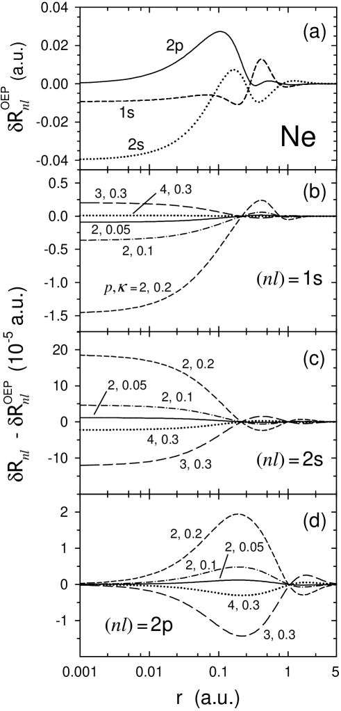
Figure 1: Approximate radial OS $\delta R_{nl}=\delta\chi_{nl}/r=\,^{[p,\kappa]}\overset{\circ}{\chi}_{nl}/r$ calculated for the Ne atom with the FD formulas for various $p,\kappa$ and compared with the exact OEP OS $\delta R_{nl}^{\text{OEP}}$, all obtained for the the exchange-only OEP density $n^{\text{OEP}}$ and the corresponding exact exchange potential $v_{\text{x}}^{\text{E}}[n^{\text{OEP}}]$ determined with the non-iterative method of Ref. CH07, .

To test one of the key elements of the present algorithm, the approximate ES $\delta\epsilon_{nl}\equiv D_{nl,nl}=\,^{[p,\kappa]}\overset{\circ}{\epsilon}_{nl}$ and radial OS $\delta R_{nl}=\,^{[p,\kappa]}\overset{\circ}{R}_{nl}$ are calculated for the exchange-only OEP density $n^{\text{OEP}}$ and the corresponding exact exchange potential $v_{\text{x}}^{\text{E}}[n^{\text{OEP}}]$ (as well as the respective orbitals and their energies) by using the FD formulas (31) and (32) with different $p$ and $\kappa$. The obtained results are compared — in Table 1 and Fig. 1 — with the exact ES and OS, i.e., $\delta\epsilon_{nl}^{\text{E}}\equiv D_{nl,nl}^{\text{OEP}}$ and $\delta R_{nl}^{\text{OEP}}$ determined with our method of Ref. CH07, . For given order $p$ of the FD formula (31), the approximate ES $\delta\epsilon_{nl}=^{[p,\kappa]}\overset{\circ}{\epsilon}_{nl}[v_{\text{x}}^{\text{E}}-\hat{v}_{\text{x}}^{\text{F}}]$ and OS $\delta R_{nl}=\,^{[p,\kappa]}\overset{\circ}{R}_{nl}[v_{\text{x}}^{\text{E}}-\hat{v}_{\text{x}}^{\text{F}}]$ become closer to $\delta\epsilon_{nl}^{\text{E}}$ and $\delta R_{nl}^{\text{E}}$ when $\kappa$ becomes smaller. For $p=1$ and $p=2$, the discrepancies $\delta\epsilon_{nl}-\delta\epsilon_{nl}^{\text{E}}$ well obey the predicted power law $\kappa^{p}$, but they decrease so quickly with increasing $p$ for each considered $\kappa=0.05,\;0.1,\;0.2$ (Table 1) that for $p=3$, $p=4$ they approach the accuracy limit, and, in consequence, their $\kappa^{p}$ dependence is not clearly seen for these $p$. The accuracy of the calculated ES $\delta\epsilon_{nl}$ (and their accuracy limit) is a combined effect of the $\kappa^{p}$ non-numerical error of the corresponding FD formula (31) and numerical inaccuracies of $\epsilon_{nl}^{\lambda}$ leading to an additional error in the ES, proportional to $1/\kappa$ (which is a factor present in FD formula (31)). Similar conclusions hold for the accuracy of the OS calculated with the FD formula (32). Hereafter, the OS and ES (as well as their increments) used in determination of $v_{\text{x}}^{[k]}$ are normally calculated with the FD formulas (31), (32) for $p=2$, $\kappa=0.05$ (invoking only two terms $\epsilon_{nl}^{\lambda}$ or $R_{nl}^{\lambda}$, with $\lambda=-\kappa,\,\kappa$), unless the dependence of the result accuracy on $p$ and $\kappa$ is studied, as in Tables 1, 3 and Fig. 1. Note that the FD formulas of higher order $p$ (3 or 4) — though requiring calculation of more terms $\epsilon_{nl}^{\lambda}$ and $R_{nl}^{\lambda}$ — should be applied when inaccuracies of these terms become larger since this adverse effect can be compensated with use of larger $\kappa$ without losing the accuracy of the resultant ES and OS.

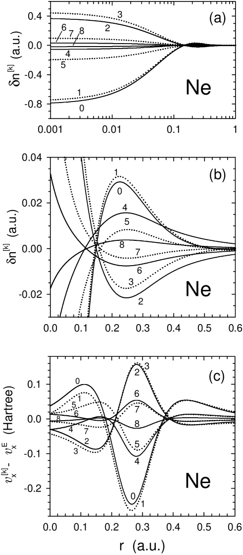
Figure 2: (a,b) Density shift $\delta n^{[k]}$ for the approximate exchange potential $v_{\text{x}}^{[k]}$ , (c) difference between $v_{\text{x}}^{[k]}$ and the exact exchange potential $v_{\text{x}}^{\text{E}}$, all obtained for the the exchange-only OEP density $n^{\text{OEP}}$ in the Ne atom. The plots are shown for $k=0,2,4,6,8$ (solid lines) and $k=1,3,5,7$ (dotted lines) and each of them is labeled with the corresponding $k$ value. For even $k$, the respective $v_{\text{x}}^{[k]}$ is obtained by modifying the OS term in $v_{\text{x}}^{[k-1]}$ while for odd $k$ it is found by $(N-1)$-parameter optimization of the ES of $v_{\text{x}}^{[k-1]}$. For better comparison with $v_{\text{x}}^{\text{E}}$ an additional constant shift is applied to $v_{\text{x}}^{[k]}$ at each iteration step $k$ to obtain $D_{NN}^{[k]}=0$, the same as $D_{NN}^{\text{E}}=0$.

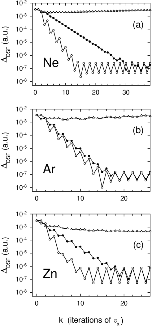
Figure 3: DSF indicator $\Delta_{\text{DSF}}^{[k]}=\|\delta n^{[k]}\|$ vs. the index $k$ of the iterative approximation $v_{\text{x}}^{[k]}$ to the exact exchange potential for the exchange-only OEP density $n^{\text{OEP}}$ in (a) Ne, (b) Ar and (c) Zn atoms. The respective $v_{\text{x}}^{[k]}$ is determined with the algorithm of Sec. VI, for even $k$ — by modifying the OS term in $v_{\text{x}}^{[k-1]}$, for odd $k$ — by the ES term modification: the $(N-1)$-parameter optimization of the ES (solid circles), the $N$-parameter optimization (open circles), no optimization, i.e., empty step (open triangles).

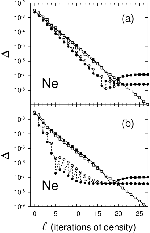
Figure 4: DSF indicators $\Delta_{\text{DSF}}^{[0]}=\|\delta n^{[0]}\|$ (open circles), $\Delta_{\text{DSF}}^{[k_{0}]}=\|\delta n^{[k_{0}]}\|$ (solid circles) and DV indicators $\Delta_{\text{DV}}^{\{\ell\},\text{OEP}}=\|n^{\{\ell\}}-n^{\text{OEP}}\|$ (solid squares), $\Delta_{\text{DV}}^{\{\ell\},\{\ell-1\}}=\|n^{\{\ell\}}-n^{\{\ell-1\}}\|$ (open squares) for consecutive approximations $n^{\{\ell\}}$ to the exchange-only OEP electron density $n^{\text{OEP}}$ in the Ne atom. The results are obtained for the approximate exchange potentials $v_{\text{x}}^{[k]}$ found — for each $n^{\{\ell\}}$ — with the algorithm of Sec. VI using $k_{0}=2$ steps in the iteration of $v_{\text{x}}^{[k]}$ and employing (a) the $(N-1)$-parameter optimization of the ES, and (b) the $N$-parameter optimization. The starting density $n^{\{0\}}$ is found with the self-consistent KLI exchange potential $v_{\text{x}}^{\text{KLI}}$. The dotted line follows the path of the the $v_{\text{x}}$ iteration.

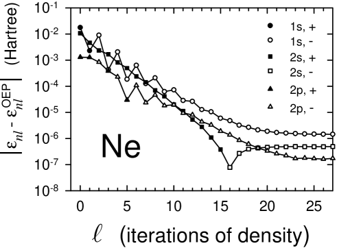
Figure 5: The absolute differences between the approximate orbital energies $\epsilon_{nl}$ obtained for the Ne atom with the KS potential $v_{\text{s}}^{\{\ell\}}$, Eq. (77), at the $\ell$-th density iteration step, and the respective energies $\epsilon_{nl}^{\text{OEP}}$ (equal to $-30.8200039329,\,-1.7181258001,\,-0.8507101622\,\text{Hartree}$ for $(nl)=1s,2s,2p$) found with the exact exchange potential for $n^{\text{OEP}}$. The exchange potential $v_{\text{x}}^{[k_{0}]}$ entering $v_{\text{s}}^{\{\ell\}}$ is found (for $n^{\{\ell-1\}}$) with $k_{0}=2$ steps of iteration which employs the $(N-1)$-parameter optimization of the ES. The results for $nl=1s$ (circles), $2s$ (squares) and $2p$ (triangles) are marked with solid symbols for positive values of $\epsilon_{nl}-\epsilon_{nl}^{\text{OEP}}$ and with open symbols for negative ones.

The efficiency of the algorithm for self-consistent determination of $n$ and $v_{\text{x}}$ has been tested for closed-(sub)shell atoms from Be to Kr and the selected results for the Ne, Ar and Zn atoms are presented in Figs. 2–5 and Tables 2, 3. The quality of the approximate exchange potential $v_{\text{x}}^{[k]}$ obtained for a given electron density ($n^{\text{OEP}}$ is used in this test) is first assessed for the Ne atom by direct comparison of $v_{\text{x}}^{[k]}$ with the exact exchange potential $v_{\text{x}}^{\text{E}}[n^{\text{OEP}}]$ (its plot is given in Fig. 1 of Ref. KP03, (a)). The iterated potential $v_{\text{x}}^{[k]}$ converges quickly to $v_{\text{x}}^{\text{E}}$ (Fig. 2(c)), so that (the maximum magnitude of) the discrepancy $\Delta v_{\text{x}}^{[k]}\equiv v_{\text{x}}^{[k]}-v_{\text{x}}^{\text{E}}$ is reduced 10, $10^{2}$, $10^{3}$ and $10^{4}$ times after $k=9,\,16,\,22,\,29$ iteration steps, respectively, in comparison to $\Delta v_{\text{x}}^{[0]}=v_{\text{x}}^{\text{KLI}}-v_{\text{x}}^{\text{E}}$ (equal to $-0.25\,\text{Hartree}$ for $r=0.26\,\text{a.u.}$). Largest discrepancies $|\Delta v_{\text{x}}^{[k]}|$ are found in the interval $0.2\,\text{a.u.}<r<0.35\,\text{a.u.}$ corresponding to the $KL$ intershell region where the characteristic bump in the $r$-dependence of $v_{\text{x}}^{\text{E}}$ is located in the Ne atom. In this region the iterated potentials $v_{\text{x}}^{[k]}$ change most significantly at even iteration steps $k$ when $v_{\text{x}}^{[k]}$ is obtained by modifying the OS term of $v_{\text{x}}^{[k-1]}$ — this leads the sign change of $\Delta v_{\text{x}}^{[k]}$ in comparison to $\Delta v_{\text{x}}^{[k-1]}$. The $(N-1)$-parameter ES optimization of $v_{\text{x}}^{[k-1]}$ — applied in this test for Ne to calculate $v_{\text{x}}^{[k]}$ at odd steps $k$ — has much smaller effect in the intershell region. However, it leads to much larger changes of the exchange potential $v_{\text{x}}^{[k]}$ for $0\leq r\leq 0.2\,\text{a.u.}$ (the $K$ shell region) which may be comparable to those induced by the OS modification at even iteration steps. The figure 2(a),(b) demonstrates that diminishing of extremal $|\delta n^{[k]}|$ is in accord with diminishing of extremal $|\Delta v_{\text{x}}^{[k]}|$, Fig. 2(c).

In practical calculations, when the exact potential $v_{\text{x}}^{\text{E}}$ is not known beforehand and thus cannot be used as a reference, the assessment of the $v_{\text{x}}^{[k]}$ quality (suggested by the comparison of Fig. 2(c) with Fig. 2(a),(b)) is done with aid of the DSF indicator $\Delta_{\text{DSF}}^{[k]}=\|\delta n^{[k]}\|$, Eq. (74), which is a suitable measure of how well the OEP equation (18a) is satisfied by $v_{\text{x}}^{[k]}$ approximating $v_{\text{x}}^{\text{E}}$. In tests for Ne, Ar, and Zn (Fig. 3), the indicator $\Delta_{\text{DSF}}^{[k]}$ calculated for a fixed density ($n^{\text{OEP}}$ is used) decreases rapidly during iteration, roughly as $ck^{-\gamma}$ ($c$, $\gamma$ — constants), until a minimum level $\Delta_{\text{DSF}}^{\text{min}}$ is reached after some number $k_{1}$ of iteration steps. This corresponds to obtaining convergence of $v_{\text{x}}^{[k]}$ for $k=k_{1}$ since $\Delta_{\text{DSF}}^{[k]}$ changes in oscillatory manner for $k>k_{1}$, with amplitude of the order of $\Delta_{\text{DSF}}^{\text{min}}$. The decrease of $\Delta_{\text{DSF}}^{[k]}$ is faster for the $N$-parameter ES optimization than for its $(N-1)$-parameter variant though the very similar $\Delta_{\text{DSF}}^{\text{min}}$ level is achieved in both cases. Its value depends on the accuracy of the ES and OS obtained with the FD formulas and it is around $10^{-7}$ for presently used $p=2$, $\kappa=0.05$ but it can be reduced below $10^{-8}$ for suitably chosen $p$, $\kappa$ (e.g., $p=2$, $\kappa=0.02$ or $p=4$, $\kappa=0.1$). The number of steps required to obtain $\Delta_{\text{DSF}}^{[k]}\approx 10^{-7}$, corresponding to convergent $v_{\text{x}}^{[k]}$ in the present test, is $k_{1}=30,\,17,\,21$ with $(N-1)$-parameter optimization and $k_{1}=13,\,13,\,11$ with $N$-parameter optimization for the Ne, Ar, and Zn atoms, respectively. However, note that the found difference in the speed of convergence of $v_{\text{x}}^{[k]}$ — especially evident, in our test, for Ne and Zn — occurs only when we consider $v_{\text{x}}^{[k]}$ calculated for a given density. This advantage of $N$-parameter ES optimization is not retained in the practical calculations when both the electron density and the exchange potential are found iteratively; see later on.

Note also that for all even $k$ the values $\Delta_{\text{DSF}}^{[k]}$ are smaller than $\Delta_{\text{DSF}}^{[k-1]}$ (see Fig. 3) since the corresponding $v_{\text{x}}^{[k]}$ are obtained by minimizing $\Delta_{\text{DSF}}$ of $v_{\text{x}}^{[k-1]}$ by treating the ES (and $D_{00}$) of this potential as $N-1$ (or $N$) variational parameters. For odd $k$, we find that $\Delta_{\text{DSF}}^{[k]}$ are often larger than $\Delta_{\text{DSF}}^{[k-1]}$, despite the mentioned overall rapid decrease of $\Delta_{\text{DSF}}^{[k]}$.

If the ES optimization is not used, the corresponding DSF indicator (marked with triangles in Fig. 3) does not decrease with $k$ (or decrease very slowly, e.g., for Zn) so that the iteration of $v_{\text{x}}^{[k]}$ does not converge. In particular, it is found that, with increasing $k$, the potential $v_{\text{x}}^{[k]}$ oscillates around $v_{\text{x}}^{\text{E}}$ in the $KL$ intershell region, changing the sign of $\Delta v_{\text{x}}^{[k]}$ after every the OS modification step, but $|\Delta v_{\text{x}}^{[k]}|$ does not decrease during iteration. This adverse behavior cannot be remedied with (often used in similar cases) mixing of the current $v_{\text{x}}$ with the one obtained in the previous step: thus the inclusion of the ES optimization step becomes essential to obtain convergence of the iterated exchange potential.

VII.3 Efficiency of present algorithm for self-consistent determination of density

Further calculations are performed using the iterations described in Sec. VI, within the exchange-only KS scheme. The convergence of the iterated density $n=n^{\{\ell\}}$ is monitored using the DV indicator $\Delta_{\text{DV}}^{\{\ell\},\{\ell-1\}}=\|n^{\{\ell\}}-n^{\{\ell-1\}}\|$. The discrepancy of $n^{\{\ell\}}$ from the exact OEP density $n^{\text{OEP}}$ is measured with another DV indicator $\Delta_{\text{DV}}^{\{\ell\},\text{OEP}}=\|n^{\{\ell\}}-n^{\text{OEP}}\|$. It is found in our test for Ne (Fig. 4) that both indicators $\Delta_{\text{DV}}^{\{\ell\},\{\ell-1\}}$, $\Delta_{\text{DV}}^{\{\ell\},\text{OEP}}$ decrease rapidly with $\ell$ (like $\ell^{-\zeta}$ where $\zeta$ – constant) and they are of the same order at each step $\ell$ of the density iteration up to $\ell=\ell_{1}=20$ where $\Delta_{\text{DV}}^{\{\ell\},\text{OEP}}$ starts to saturate at a very small value of the order of $10^{-7}$. Therefore, a further decrease of $\Delta_{\text{DV}}^{\{\ell\},\{\ell-1\}}$ for $l>l_{1}$, seen in Fig. 4, and indicating a seemingly better convergence of $n^{\{\ell\}}$, is not accompanied by further improving of the density (lowering of $\Delta_{\text{DV}}^{\{\ell\},\text{OEP}}$) for $l>l_{1}$. Similar $\ell$-dependence of the DV indicators is found for other closed-shell atoms. Thus, we conclude that the DV indicator $\Delta_{\text{DV}}^{\{\ell\},\{\ell-1\}}$ is a suitable tool to assess the quality of the consecutive approximations $n^{\{\ell\}}$ to $n^{\text{OEP}}$, provided that $\ell\leq\ell_{1}$. In practice, the value of $\ell_{1}$ is close to the crossing point of the $\Delta_{\text{DV}}^{\{\ell\},\{\ell-1\}}$ vs $\ell$ line with the $\Delta_{\text{DSF}}^{[0]}$ vs $\ell$ line; see discussion below. With this definition, we find $\ell_{1}=21,\,20,\,17$ for Ne, Ar, Zn.

In the reported test for the Ne atom, the exchange potential is calculated using only $k_{0}=2$ iteration steps for each approximate density $n=n^{\{\ell\}}$. Despite so small $k_{0}$, the DSF indicator $\Delta_{\text{DSF}}^{[0]}$ decays quickly, like $\ell^{-\zeta_{1}}$ (where $\zeta_{1}$ — constant) with increasing $\ell$ during the density iteration and it approaches a limiting value, less than $10^{-7}$, after some number of steps close to $\ell_{1}$ (but, a few steps earlier for other atoms, like Ar and Zn). The partner indicator $\Delta_{\text{DSF}}^{[k_{0}]}$ reaches the same limiting level in the same range of $\ell$.

The speed of convergence of iterated density does not depend on the type of the ES optimization used in calculation of $v_{\text{x}}$, as it is seen in Fig. 4(a),(b) for Ne and in Table 2 for Zn. It is also found that increasing the number $k_{0}$ of steps in the iteration of the exchange potential — although leading to smaller $\Delta_{\text{DSF}}^{[k_{0}]}$ for each density $n^{\{\ell\}}$ — does not accelerates the overall convergence in the density iteration. In the test for Zn (Table 2), the DV indicator $\Delta_{\text{DV}}^{\{\ell\},\text{OEP}}$ obtained for $k_{0}\geq 3$ is even slightly larger, than for $k_{0}=2$; it is true for each $\ell>0$ and both types of the ES optimization. Thus, $k_{0}=2$ and $(N-1)$-parameter ES modification is recommended as an optimal choice.

Summarizing the discussion on the use of the DSF and DV indicators we conclude that the condition (78), with suitably chosen accuracy thresholds $\eta_{\text{DSF}}$ and $\eta_{\text{DV}}$, can indeed be used for termination of the combined iteration of $n^{\{\ell\}}$ and $v_{\text{x}}^{[k]}$. In particular, in the discussed test for Ne (with $k_{0}=2$ and the $(N-1)$-parameter ES optimization) choosing $\eta_{\text{DSF}}=\eta_{\text{DV}}=10^{-4},\,10^{-5},\,10^{-6},\,10^{-7}$ leads to termination after, respectively, $\ell=6,\,10,\,15,\,20$ steps of the density iteration while the resultant $n^{\{\ell\}}$ becomes increasingly accurate since we find $\Delta_{\text{DV}}^{\{\ell\},\text{OEP}}\approx\Delta_{\text{DV}}^{\{\ell\},\{\ell-1\}}\approx\eta_{\text{DV}}$.

The occupied orbital energies $\epsilon_{nl}$, obtained with the KS potential $v_{\text{s}}^{\{\ell\}}$ at consecutive iteration steps $\ell$, converge to the corresponding OEP values $\epsilon_{nl}^{\text{OEP}}$ at similar speed as $\Delta_{\text{DV}}^{\{\ell\},\text{OEP}}$. For the Ne atom (Fig. 5), the discrepancies $|\epsilon_{nl}-\epsilon_{nl}^{\text{OEP}}|$ decrease with $\ell$ roughly as $\ell^{-\zeta}$ (i.e., with similar exponential decay as $\Delta_{\text{DV}}^{\{\ell\},\text{OEP}}$) and saturate at around the $10^{-6}-10^{-7}\,\text{Hartree}$ level after a number of steps close to $\ell_{1}=21$. Note that $\epsilon_{nl}$ may oscillate around $\epsilon_{nl}^{\text{OEP}}$ during iteration, which leads to changing the sign of $\epsilon_{nl}-\epsilon_{nl}^{\text{OEP}}$, like for $(nl)=2p$ orbital in the Ne atom.

The discrepancy of $\epsilon_{nl}$ from $\epsilon_{nl}^{\text{OEP}}$ becomes less than $10^{-4}\,\text{Hartree}$ for all occupied orbitals $nl$ after 9 density iterations for Ne, and 12 steps for Ar and Zn while using only $k_{0}=2$ steps in iteration of $v_{\text{x}}$ for each density. Thus, the 0.1 mHartree accuracy of orbital energies is obtained after a similar number of iterations as in Ref. KP03, , where a different method of $v_{\text{x}}$ iteration is applied and the OS are found by solving the KP differential equations.

The accuracy of calculated energies $\epsilon_{nl}$ depends on the choice of $p$ and $\kappa$ in the FD formulas (31), (32) used to determine the approximate ES and OS applied in the iteration of $v_{\text{x}}$. Indeed, in the test for Zn (Table 3), the discrepancy of $\epsilon_{nl}$ from $\epsilon_{nl}^{\text{OEP}}$ decreases rapidly with $\kappa$, especially for $p=3,\,4$. The discrepancy magnitudes depend on $\kappa$ roughly as $\kappa^{p}$ so that they obey the same power law as the ES and OS errors corresponding to the type of the FD formula applied in the calculations. The accuracy of the occupied orbital energies obtained for Zn is $10^{-5}$ and $10^{-6}$ Hartree for $p=2,\kappa=0.05$ and $p=4$, $\kappa=0.1$, while it reaches $10^{-7}\,\text{Hartree}$ for $p=4$, $\kappa=0.05$. Note that the choice of $p$, $\kappa$, though determining the final accuracy of $\epsilon_{nl}$, does not affect the rate of convergence of the orbital energies during density iteration.

VIII Conclusions

The performed calculations for closed-(sub)shell atoms prove that the exact exchange potential can be determined very accurately with the presently proposed algorithm using only the occupied solutions of the perturbed KS equations. Since the respective perturbation is given by the (scaled) DFT exchange potential or the (scaled) difference between this potential and the non-local Fock exchange operator (built with the KS orbitals), the perturbed KS equations have a similar form as the KS or HF equations. Thus, these KS-like and HF-like equations can be solved with (only slightly modified) standard numerical methods applicable to the KS and HF equations. Therefore, the present algorithm for determination of the exact exchange potential, shown in this work to be effective and very accurate in the spatial-grid representation (with the pseudospectral method), is plausibly suitable for its implementation within standard codes using an orbital basis to represent the KS orbitals as well as the KS-like and HF-like orbitals applied in the iteration of $v_{\text{x}}$.

The applied method of iterating the exchange potential, which is the second new element of our algorithm, is found to be convergent only if the modification of its OS term, performed at even iteration steps, is accompanied by the optimization of the ES term at odd steps. With both ES and OS modifications included, the rapid convergence of the obtained DS norm, decreasing below $10^{-6}$ in less than 20 iteration steps, proves high efficiency of the algorithm and very high accuracy of $v_{\text{x}}$ at convergence (as the DS norm vanishes for exact $v_{\text{x}}$ due to the OEP equation). Since the iteration of the exchange potential can be reduced to only 2 steps (for each density) in the self-consistent density calculations within the exchange-only KS scheme, without affecting the quick convergence of the iterated density, the orbital energies of $10^{-6}-10^{-7}\,\text{Hartree}$ accuracy are obtained for atoms with only the total number of $20\times 2=40$ iterations of $v_{\text{x}}$ (starting with the KLI approximation).

Finally, we expect that the proposed algorithm for determination of the exact exchange potential, successfully tested in calculations for atoms in a spatial-grid representation, should also be equally efficient for molecules, and that it could be applied within an orbital-basis representation.

Appendix A Reduction of $N$-dimensional algebraic problem
to $(N-1)$-dimensional one

The $N$-dimensional system of algebraic equations for unknown ${\bf{\sf d}}^{{}^{\prime}}$, represented by a matrix equation

$${\bf{\sf A}}^{{}^{\prime}}\,{\bf{\sf d}}^{{}^{\prime}}={\bf{\sf b}}^{{}^{\prime}}$$ (80)

where ${\bf{\sf A}}^{{}^{\prime}}$ is $N\times N$ square symmetric matrix $\{A_{ac}\}_{a,c=0}^{N-1}$, while ${\bf{\sf d}}^{{}^{\prime}}$ and ${\bf{\sf b}}^{{}^{\prime}}$ are $N\times 1$ column matrices $\{d_{c}\}_{c=0}^{N-1}$ and $\{b_{c}\}_{c=0}^{N-1}$, can be rewritten equivalently as a system of the following two equations

$$A_{00}\,d_{0}+{\bf{\sf A}}_{0}^{\text{{\sf T}}}\,{\bf{\sf d}} = b_{0}\,,$$ (81)

$${\bf{\sf A}}\,{\bf{\sf d}}+{\bf{\sf A}}_{0}\,d_{0} = {\bf{\sf b}}\,,$$ (82)

where ${\bf{\sf A}}$ is $(N-1)\times(N-1)$ square matrix $\{A_{ac}\}_{a,c=1}^{N-1}$, ${\bf{\sf d}}$, ${\bf{\sf b}}$ and ${\bf{\sf A}}_{0}$ are $(N-1)\times 1$ column matrices $\{d_{c}\}_{c=1}^{N-1}$, $\{b_{c}\}_{c=1}^{N-1}$, $\{A_{c0}\}_{c=1}^{N-1}$, while $A_{00}$, $d_{0}$ and $b_{0}$ are separate elements. The solution of the system of Eqs. (81) and (82) is found to be

$$d_{0}=\frac{b_{0}-{\bf{\sf A}}_{0}^{\text{{\sf T}}}\,{\bf{\sf A}}^{-1}\,{\bf{\sf b}}}{A_{00}-{\bf{\sf A}}_{0}^{\text{{\sf T}}}\,{\bf{\sf A}}^{-1}\,{\bf{\sf A}}_{0}}\,,$$ (83)

$${\bf{\sf d}}={\bf{\sf A}}^{-1}\,({\bf{\sf b}}-{\bf{\sf A}}_{0}\,d_{0})\,.$$ (84)

As we see, for its evaluation it is sufficient to determine the $(N-1)\times(N-1)$ matrix ${\bf{\sf A}}^{-1}$ instead of the $N\times N$ matrix $\bigl{(}{\bf{\sf A}}^{{}^{\prime}}\bigr{)}^{-1}$, necessary in the case of direct solution of the original Eq. (80). And what is more, in our application the matrix ${\bf{\sf A}}^{-1}$ is common for all steps of iterations at fixed density, while the matrix $\bigl{(}{\bf{\sf A}}^{{}^{\prime}}\bigr{)}^{-1}$ is specific to each step separately.

Table 1: The approximate ES $\delta\epsilon_{nl}=\,^{[p,\kappa]}\overset{\circ}{\epsilon}_{nl}$ obtained with the FD formulas (31) for various $p\,,\kappa$. The calculations use the exchange-only OEP density $n^{\text{OEP}}$ in the Ne atom and the corresponding exact exchange potential $v_{\text{x}}^{\text{E}}=v_{\text{x}}^{\text{E}}[n^{\text{OEP}}]$, both determined with the non-iterative method of Ref. CH07, . The shown values are discrepancies of $\delta\epsilon_{nl}$ from the ES $D_{nl,nl}^{\text{OEP}}=D_{nl,nl}[v_{\text{x}}^{\text{E}}]$ (given in the last row).

		$\delta\epsilon_{nl}-D_{nl,nl}^{\text{OEP}}$ $\;\;(10^{-4}\text{Hartree})$
$p$	$\kappa$	$\;\;(nl)\,=\;1s$	$\;\;\;2s$	$\;\;2p$
$1$	$0.2$	$-0.811010$	$-0.182120$	$-0.245732$
$1$	$0.1$	$-0.403044$	$-0.090118$	$-0.122396$
$1$	$0.05$	$-0.200911$	$-0.044839$	$-0.061091$
$2$	$0.2$	$-0.009635$	$-0.003484$	$-0.001826$
$2$	$0.1$	$-0.002408$	$-0.000879$	$-0.000458$
$2$	$0.05$	$-0.000601$	$-0.000220$	$-0.000116$
$3$	$0.2$	$0.000282$	$0.000435$	$0.000086$
$3$	$0.1$	$0.000035$	$0.000049$	$0.000008$
$3$	$0.05$	$0.000006$	$0.0000002$	$-0.000006$
$4$	$0.2$	$0.000008$	$0.000054$	$0.000010$
$4$	$0.1$	$0.0000003$	$0.000004$	$-0.000002$
$4$	$0.05$	$0.000001$	$-0.000004$	$-0.000002$
$D_{nl.nl}^{\text{OEP}}$		$1.950\,526\,191\,9$	$0.210\,906\,681\,7$	$\;0$
$\;\;(\text{Hartree})$

Table 2: The indicator $\Delta_{\text{DV}}^{\{\ell\},\text{OEP}}=\|n^{\{\ell\}}-n^{\text{OEP}}\|$ of the discrepancy between the approximate electron density $n^{\{\ell\}}$ at the $\ell$-th iteration step and the exchange-only OEP density $n^{\text{OEP}}$ for the Zn atom. The shown results are obtained for each density $n^{\{\ell\}}$ with $k_{0}$ steps in the iteration of the exchange potential $v_{\text{x}}^{[k]}$ and either $(N-1)$- or $N$-parameter ES optimization.

	$\Delta_{\text{DV}}^{\{\ell\},\text{OEP}}$ $\;\;(\times 10^{-3})$
	$(N-1)$-parameter			$N$-parameter
$\ell$	$k_{0}=2$	$k_{0}=3$	$k_{0}=7$	$k_{0}=2$	$k_{0}=3$	$k_{0}=7$
0	3.07390	3.07390	3.07390	3.07390	3.07390	3.07390
1	1.27749	1.71563	1.82028	1.27749	1.84049	1.83820
2	0.95047	1.06142	1.07960	0.79210	1.09074	1.08965
3	0.49044	0.61554	0.64348	0.46845	0.65009	0.64967
5	0.17837	0.21939	0.22823	0.16534	0.23049	0.23052
10	0.01355	0.01659	0.01724	0.01242	0.01739	0.01742
20	0.00049	0.00060	0.00060	0.00049	0.00060	0.00060
30	0.00047	0.00057	0.00057	0.00047	0.00057	0.00057

Table 3: The orbital energies $\epsilon_{nl}$ vs. $p\,,\kappa$ for the Zn atom obtained — after 25 iterations of $n^{\{\ell\}}$ — with the algorithm of Sec. VI using $k_{0}=2$ iteration steps and $(N-1)$-parameter ES optimization in determination of the exchange potential $v_{\text{x}}^{[k]}$ for each $n^{\{\ell\}}$. The applied OS and ES are found with the FD formulas (31), (32) using the chosen $p\,,\kappa$. The shown values are discrepancies of $\epsilon_{nl}$ from the orbital energies $\epsilon_{nl}^{\text{OEP}}$ (given in the last row) calculated with the exact exchange potential $v_{\text{x}}^{\text{E}}[n^{\text{OEP}}]$ determined with the non-iterative method of Ref. CH07, .

		$\epsilon_{nl}-\epsilon_{nl}^{\text{OEP}}$ $\;\;(10^{-4}\text{Hartree})$
$p$	$\kappa$	$(nl)\,=\;\;1s$	$2s$	$3s$	$4s$	$2p$	$3p$	$3d$
1	$0.2$	$-10.640$	$-9.992$	$-12.802$	$3.106$	$-8.231$	$-12.603$	$-10.352$
1	$0.1$	$-5.192$	$-4.714$	$-6.001$	$1.474$	$-3.813$	$-5.889$	$-4.808$
1	$0.05$	$-2.575$	$-2.296$	$-2.912$	$0.719$	$-1.842$	$-2.853$	$-2.323$
2	$0.2$	$-0.056$	$-1.075$	$-1.885$	$0.308$	$-0.981$	$-1.957$	$-1.816$
2	$0.1$	$-0.019$	$-0.268$	$-0.466$	$0.077$	$-0.246$	$-0.484$	$-0.449$
2	$0.05$	$-0.005$	$-0.066$	$-0.116$	$0.019$	$-0.061$	$-0.121$	$-0.112$
3	$0.2$	$0.126$	$0.661$	$0.927$	$-0.131$	$0.640$	$0.963$	$0.914$
3	$0.1$	$0.010$	$0.065$	$0.091$	$-0.013$	$0.062$	$0.095$	$0.090$
3	$0.05$	$0.001$	$0.009$	$0.011$	$-0.002$	$0.007$	$0.011$	$0.010$
4	$0.2$	$0.041$	$0.170$	$0.225$	$-0.031$	$0.165$	$0.233$	$0.222$
4	$0.1$	$0.002$	$0.011$	$0.013$	$-0.002$	$0.010$	$0.013$	$0.013$
4	$0.05$	$-0.0005$	$0.0015$	$0.0007$	$-0.0004$	$0.0006$	$0.0005$	$0.0007$
$\epsilon_{nl}^{\text{OEP}}$		$-345.755720523$	$-41.714189169$	$-4.796168733$	$-0.292805644$	$-36.742098912$	$-3.210661901$	$-0.537803838$
$\;\;(\text{Hartree})$

References

- (1) P. Hohenberg and W. Kohn, Phys. Rev. 136, B864 (1964).
- (2) R. G. Parr, W. Yang, Density-Functional Theory of Atoms and Molecules (Oxford University Press, Oxford, 1989).
- (3) R. M. Dreizler, E. K. U. Gross, Density Functional Theory (Springer, Berlin, 1990).
- (4) D. R. Salahub, A. Goursot, J. Weber, A. M. Köster and A. Vela, in Theory and Applications of Computational Chemistry: The First Forty Years, edited by C. E. Dykstra, G. Frenking, K. S. Kim and G. E. Scuseria, (Elsevier, Amsterdam, 2005), p. 1079.
- (5) J. P. Perdew and S. Kurth, in A Primer in Density Functional Theory, edited by C. Fiolhais, F. Nogueira, M. Marques, Lecture Notes in Physics 620 (Springer, Berlin, 2003), p. 1.
- (6) T. Kreibich, S. Kurth, T. Grabo, and E. K. U. Gross, Adv. Quantum Chem. 33, 31 (1999).
- (7) J. D. Talman and W. F. Shadwick, Phys. Rev. A 14, 36 (1976).
- (8) Y. Wang, J. P. Perdew, J. A. Chevary, L. D. Macdonald, and S. H. Vosko, Phys. Rev. A 41, 78 (1990).
- (9) J. B. Krieger, Y. Li, and G. J. Iafrate, Phys. Rev. A 45, 101 (1992); ibid. 46, 5453 (1992).
- (10) E. Engel, as in PK03 , p. 56.
- (11) A. Görling and M. Levy, Phys. Rev. A 50, 196 (1994).
- (12) A. Görling and M. Levy, Phys. Rev. B 47, 13105 (1993).
- (13) Y. Li, J. B. Krieger, and G. J. Iafrate, Phys. Rev. A 47, 165 (1993).
- (14) E. Engel and S. H. Vosko, Phys. Rev. A 47, 2800 (1993).
- (15) E. Engel, and and R. M. Dreizler, J. Comp. Chem. 20, 31 (1999).
- (16) E. Engel, A. Höck, and R. M. Dreizler, Phys. Rev. A 62, 042502 (2000), ibid. 63, 039901 (2001) (E).
- (17) A. Görling, Phys. Rev. Lett. 83, 5459 (1999).
- (18) S. Ivanov, S. Hirata, and R. J. Bartlett, Phys. Rev. Lett. 83, 5455 (1999).
- (19) S. Hirata, S. Ivanov, I. Grabowski, and R. J. Bartlett, K. Burke, and J. D. Talman, J. Chem. Phys. 115, 1635 (2001).
- (20) F. Della Sala and A. Görling, J. Chem. Phys. 115, 5718 (2001).
- (21) A. Heßelmann, A. W. Götz, F. Della Sala, and A. Görling, J. Chem. Phys. 127, 054102 (2007).
- (22) V. N. Staroverov, G. E. Scuseria, and E. R. Davidson, J. Chem. Phys. 124, 141103 (2006).
- (23) T. Heaton-Burgess, F. A. Bulat, and W. Yang, Phys. Rev. Lett. 98, 256401 (2007).
- (24) T. Heaton-Burgess and W. Yang, J. Chem. Phys. 129, 194102 (2008).
- (25) A. Görling, A. Heßelmann, M. Jones and M. Levy, J. Chem. Phys. 128, 104104 (2008).
- (26) W. Yang and Q. Wu, Phys. Rev. Lett. 89, 143002 (2002).
- (27) J. J. Fernandez, C. Kollmar, and M. Filatov, Phys. Rev. A 82, 022508 (2010).
- (28) S. Kümmel and J. P. Perdew, Phys. Rev. Lett. 90, 043004 (2003), Phys. Rev. B 68, 035103 (2003).
- (29) T. Grabo, T. Kreibich, S. Kurth and E. K. U. Gross, in Strong Coulomb Correlations in Electronic Structure Calculations: Beyond the Local Density Approximation, edited by V. I. Anisimov, (Gordon and Breach, 2000), pp. 203–311.
- (30) M. Cinal and A. Holas, Phys. Rev. A 76, 042510 (2007).
- (31) S. Kümmel and L. Kronik, Rev. Mod. Phys. 80, 3 60 (2008).
- (32) A. Holas and M. Cinal, Phys. Rev. A 72, 032504 (2005).
- (33) M. Cinal, J. Chem. Phys. 132, 014101 (2010).
- (34) F. Della Sala and A. Görling, (a) Phys. Rev. Lett. 89, 033003 (2002); (b) J. Chem. Phys. 116, 5374 (2002).
- (35) J. Wang, Shih-I Chu, and C. Laughlin, Phys. Rev. A 50, 3208 (1994).
- (36) A. K. Roy and Shih-I Chu, Phys. Rev. A 65, 052508 (2002).
- (37) R. A. Friesner, Chem. Phys. Lett. 116, 39 (1985).
- (38) R. A. Friesner, J. Chem. Phys. 85, 1462 (1986).
- (39) M. Cinal, in preparation.