Tailoring photon emission patterns in nanostructures

Abstract

We investigate the photon emission in coupled quantum dots based on symmetry considerations. With the help of a new theorem we proved, we reveal the origin of the various emission patterns, which is the combinative symmetry in the time domain and spectrum domain. We are able to tailor the emission patterns and obtain emission spectra with odd harmonics only, even harmonics only, both odd and even harmonic components, or even the quenching of all components. These interesting emission patterns can be obtained in experiments by careful design of the nanostructures, which are of many applications in optical-electric nanodevices.

I Introduction

Photon emission in nanostructures plays a crucial role in modern electronic/optical devices. Generating high-order harmonics is one efficient up-conversion method for obtaining desired spectra (for example, THz spectra) from sources with lower frequencies. During the last several decades, much effort was made in the study of generation of high-order harmonics in atomic/molecular systems and nanostructures 1Ahn2007PRL ; 2Chassagneux2009Nature ; 3zhang2009PRB ; agdot04 ; terzis ; moiseyev2001 , as well as their applications. For instance, Ahn et al recently proposed an approach for THz wave generation by high-order harmonic wave based on semiconductor nanostructures driven by acoustic wave 1Ahn2007PRL . A scheme of electrically pumped photonic-crystal THz laser 2Chassagneux2009Nature was developed by Chassagneux et al. A method for THz wave generation by Gigahertz wave was also suggested in 3zhang2009PRB .

Different harmonic components have interesting applications. For example, even harmonics were used as a test wave to diagnose the fast time evolution of the current density 4Ferrante2005PLA . Yet odd harmonics were often observed in experiments in atomic and molecular systems. The appearance of odd harmonics was attributed to the particular inversion symmetry in central potential. There have been several studies on the dynamical symmetry symmetry and related selection rules select in high-order harmonics generation. People have tried to get even harmonics by avoiding the selection rule 5Xie2002PRA ; 6Ferrante2004PLA ; 8Pietro2007MO ; 9Bavli1993PRA ; 10Thomas2001PRL . Some studies focused on the symmetry breaking for obtaining the even harmonics in molecules and atoms 9Bavli1993PRA ; 10Thomas2001PRL ; 8Pietro2007MO . The symmetry breaking may be realized in the molecule with two nucleus of different masses10Thomas2001PRL . The even harmonics were found to appear in driven double quantum wells, where the potential was not of inversion symmetry. Also the radiation may occur at non-integer multiples of the fundamental frequency.

There have been many theoretical and experimental studies on high-order harmonics, and most of them focused on the atomic and molecular systems 11Wu2008OLA ; 12Zhou2008PRA ; 13Heslar2007IJQC ; 14Le2007PRA ; 15F2006PRL ; 16McPherson1987OSAB ; 17Huillier1991PhysB ; 18Protopapas1997RPP ; 19Salieres1999AAMOP ; 20Chang1997PRL ; 21Schnurer1998PRL ; 22Salieres1998PRL ; corso98 . In spite of many studies on even harmonics generation, it appears that the deep origin of different emission patterns is still unclear, and an effective way of generating emission spectra of specific pattern is lack. In this paper, we study the emission spectra of coupled quantum dots (QDs), and find the symmetry origin of various emission patterns, as well as methods for generating different emission patterns including those with even harmonics. The main advantage of QD (artificial atom) and coupled quantum dots (CQDs) (artificial molecules) is their tunability. By carefully designing the material, the growth process, or adding appropriate gate voltages etc., one is able to adjust the energy levels/energy gaps in CQDs. One can further design the structure of CQDs (the relative position of QDs, the inter-dot distances, the hight and width of the tunneling barriers) to tune the optical dipole between QDs. The optical coupling between QDs can also be changed by tuning the polarization of the incident light. Compared with one quantum dot with multiple energy levels, the CQD system has the advantage of more tunability. By making full use of the tunability of coupled nanostructures, we propose an effective approach to tailor emission patterns. We reveal the origin of appearance of odd/enen harmonics based on the symmetry considerations. It turns out that the emission pattern is determined not just by the inverse symmetry, but by a new type of symmetry, which is the combinative symmetry in the time domain and spectrum domain. Based on our findings, we are able to obtain emission patterns with even harmonics only, odd harmonics only, or both even and odd harmonics, and even disappearance of all harmonic components. Our methods of generation of various emission patterns in nanostructures have important applications.

II THEORETICAL FORMULISM

We consider a CQD system with one energy level for each dot. The energy is $E_{i}$ for the state $|i\rangle$ in the dot $i$, $i=1...N$. This CQD is driven by an external field $E=F\cos(\omega_{0}t){\vec{u}}$, ${\vec{u}}$ unit vector.

Under the dipole approximation, our system is described by the Hamiltonian

$$H=\sum_{i}E_{i}|i\rangle\langle i|+\sum_{i\neq j}G_{ij}\cos(\omega_{0}t)|i\rangle\langle j|,$$ (1)

where $G_{ij}=F{\vec{u}}\cdot{\vec{\mu}_{ij}}$ are Rabi frequencies, ${\vec{\mu}_{ij}}=\langle i|e{\vec{r}}|j\rangle$ the dipole between dot $i$ and dot $j$. The equation of motion for the density matrix is written in the form 23Narducci1990PRA

$$\frac{\partial\rho}{\partial t}=-\frac{i}{\hbar}[H,\rho]-\Gamma\cdot\rho,$$ (2)

where the last term describes possible dissipation effects (for instance that from the spontaneous phonon emission). We set $\hbar=1$ in the following. The time-dependent mean dipole moment can be calculated as $P(t)=\langle er\rangle=\sum_{ij}\mu_{ij}\rho_{ij}(t)$. With the help of Fourier transformation we can obtain the emission spectrum $S(\omega)=|\int dt\exp(i\omega t)P(t)|^{2}$. Now we present a theorem on the origin of the various emission patterns. Several examples will be given.

Theorem For a quantum system described by the Hamiltonian (1), if there exists one symmetric operation Q, which is the time shift $\theta:t\rightarrow t+T/2$ (or $-t+T/2$, $T=2\pi/\omega_{0}$) combined with another operation $\Omega$ in spatial/spectrum domain, i.e. $Q=\Omega\cdot\theta\$, such that the initial condition and the Hamiltonian are invariant (or $H\rightarrow-H$), and the dipole operator $\hat{P}$ has a definite parity, then the emission spectrum contains no odd/even component if operator $\hat{P}$ is even/odd.

The proof goes as following:

Proof We first consider the case: under the operation Q, $H$ $\rightarrow$ $H$. The schrodinger equation $i\frac{d}{dt}|\psi\rangle=H|\psi\rangle$ remains invariant under Q transformation. If the initial condition remains unchanged (up to a phase), that is, the initial condition $|\psi(t=0)\rangle$ satisfies $|\widetilde{\psi}(t=0)\rangle\equiv Q|{\psi}(t=0)\rangle=e^{-i\gamma}|{\psi}(t=0)\rangle$, then we have $|\widetilde{\psi}(t)\rangle=e^{-i\gamma}|{\psi}(t)\rangle$. Therefore $P(t)=\langle\psi(t)|\hat{P}|\psi(t)\rangle=\langle\widetilde{\psi(t)}|\hat{P}|\widetilde{\psi(t)}\rangle=\langle\psi(t+T/2)|\Omega^{-1}\hat{P}\Omega|\psi(t+T/2)\rangle=\langle\psi(t+T/2)|\pm\hat{P}|\psi(t+T/2)\rangle=\pm P(t+T/2)$, where ”+” for even $\hat{P}$ and ”-” for odd $\hat{P}$. Thus we have $P(n\omega_{0})\equiv\int dte^{in\omega_{0}t}P(t)=\pm\int dte^{in\omega_{0}(t-T/2)}P(t)=\pm(-1)^{n}P(n\omega_{0})$.

Similarly for the case: under the operation Q, $H$ $\rightarrow$ $-H$. $P(t)=\langle\psi(t)|\hat{P}|\psi(t)\rangle=\langle\widetilde{\psi(t)}|\hat{P}|\widetilde{\psi(t)}\rangle=\langle\psi(-t+T/2)|\Omega^{-1}\hat{P}\Omega|\psi(-t+T/2)\rangle=\langle\psi(-t+T/2)|\pm\hat{P}|\psi(-t+T/2)\rangle=(\langle\psi(t-T/2)|)^{*}\pm\hat{P}(|\psi(t-T/2)\rangle)^{*}=\langle\psi(t-T/2)|\pm\hat{P}|\psi(t-T/2)\rangle=\pm P(t-T/2)$, where we have used the fact that $P(t)$ is real. Thus we also have $P(n\omega_{0})=\pm(-1)^{n}P(n\omega_{0})$.

So we reach the results,

$P(n\omega_{0})=0$ for odd n, if $\hat{P}$ is even (under $\Omega$);

$P(n\omega_{0})=0$ for even n, if $\hat{P}$ is odd (under $\Omega$).

From above proof, one sees that the required initial condition is $|\psi(t=0)\rangle=e^{i\gamma}Q|\psi(t=0)\rangle=e^{i\gamma}\Omega|\psi(T/2)\rangle=e^{i\gamma}\Omega U(T/2)|\psi(0)\rangle$, where U is the time evolution operator. So the initial state needs to be an eigenvector of the operator $\Omega U(T/2)$. This initial condition is not very convenient for practical use since the time evolution operator is involved. Here we demonstrate that the initial condition could be replaced with $|\psi(t=0)\rangle=e^{i\gamma}\Omega|\psi(t=0)\rangle$, and the emission spectra have little change, as long as $|E_{i}-E_{j}|/\omega_{0}$ is small.

Physically we can understand that for linear time evolution systems, very small change of initial condition does not lead to big change of the time evolution of the system. More precisely, from Floquet theorem, we have $|\psi(t)\rangle=\sum_{\alpha}c_{\alpha}e^{-i\varepsilon_{\alpha}t}|u_{\alpha}(t)\rangle$, with $|u_{\alpha}(t)\rangle$ the time periodic Floquet state, $c_{\alpha}$ determined by the initial condition. It is easy to see that $P(\omega)=\sum_{\alpha,\alpha^{\prime}}c^{*}_{\alpha^{\prime}}c_{\alpha}K_{\alpha,\alpha^{\prime}}(\omega)$, where $K_{\alpha,\alpha^{\prime}}(\omega)=\int dte^{i\omega t}e^{-i(\varepsilon_{\alpha}-\varepsilon_{\alpha}^{\prime})t}u^{*}_{\alpha^{\prime}}(t)\hat{P}u_{\alpha}(t)$. So for two different initial conditions with $c_{\alpha},\widetilde{c}_{\alpha}$, such that $|c_{\alpha}-\widetilde{c}_{\alpha}|<\eta$, $\eta$ a sufficient small parameter, it is easy to show that $|P(\omega)-\widetilde{P}(\omega)|<\sum_{\alpha,\alpha^{\prime}}2\eta K_{\alpha,\alpha^{\prime}}$, here $P(\omega),\widetilde{P}(\omega)$ are the emission spectra corresponding to the initial conditions with $c_{\alpha}$, $c_{\alpha}^{\prime}$ respectively.

Now we show that the difference between the initial conditions satisfying $|\psi(t=0)\rangle=e^{i\gamma}\Omega|\psi(t=0)\rangle$ and $|\psi(t=0)\rangle=e^{i\gamma}Q|\psi(t=0)\rangle$ can be small enough, if $|E_{i}-E_{j}|/\omega_{0}\ll 1$. The time evolution operator satisfies the equation $idU/dt=\hat{H}U$ with initial condition $U(t=0)=I$, $I$ the identical operator. $\hat{H}=\hat{E}+G\cos(\omega_{0}t)\hat{\mu}$, where $\hat{E}=diag(E_{1},...,E_{N})$. The symmetric matrix $\hat{\mu}$ can be diagonalized as $A^{-1}\hat{\mu}A=diag(\lambda_{1},...\lambda_{N})$. Using the transformation $U=AB\bar{U}A^{-1}$, $B=diag(e^{-i\lambda_{1}Gf(t)},...,e^{-i\lambda_{N}Gf(t)})$, $f(t)=\int_{0}^{t}d\tau\cos(\omega_{0}\tau)$, one sees that $id\bar{U}/dt=\bar{E}\bar{U}$, where $\bar{E}=B^{-1}A^{-1}\hat{E}AB$, $\bar{U}(t=0)=I$. Then it is clear that $|\bar{U}(T/2)-I|$ and $|{U(T/2)}-I|=|A[\bar{U}(T/2)-I]A^{-1}|$ can be small enough, if $|E_{i}-E_{j}|/\omega_{0}$ is small. Since $Q=\Omega U(T/2)=\Omega+\Omega U(T/2)-\Omega=\Omega+\Omega(U(T/2)-I)$, standard perturbative calculation shows that the correction of initial condition due to perturbation $\Omega(U(T/2)-I)$ is small and one can use the initial condition $|\psi(t=0)\rangle=e^{i\gamma}\Omega|\psi(t=0)\rangle$ for the cases with $|E_{i}-E_{j}|/\omega_{0}\ll 1$. In the above proof the dissipation hasn’t been included, yet we would like to point out that if the dissipation is small, the main feature of emission spectra remains unchanged as verified by our numerical calculations shown in the next section.

We have obtained one selection rule in the perturbation regime ( $|E_{i}-E_{j}|/\omega_{0}\ll 1$) and it depends on the initial condition. What may happen in the nonperturbation regime? In the regime with large $|E_{i}-E_{j}|/\omega_{0}$ and $G/\omega_{0}$, most quasienergies are large and the corresponding quasienergy states in the expansion $|\psi(t)\rangle=\sum_{\alpha}c_{\alpha}e^{-i\varepsilon_{\alpha}t}|u_{\alpha}(t)\rangle$ lead to fast oscillation behavior, only the quasienergy state with the smallest quasienergy $\varepsilon_{\alpha_{0}}$ (modulo $\hbar\omega_{0}$) dominates, i.e., $|\psi(t)\rangle=c_{\alpha_{0}}e^{-i\varepsilon_{\alpha_{0}}t}u_{\alpha_{0}}(t)$. If there exists one symmetric operation $Q$ such that $QHQ^{-1}=H$, $Qi\frac{d}{dt}Q^{-1}=i\frac{d}{dt}$, then the state $Q|u_{\alpha_{0}}\rangle$ is also a quasienergy state with quasienergy $\varepsilon_{\alpha_{0}}$. If the quasienergy states are nondegenerate, $Q|u_{\alpha_{0}}\rangle$ is just $|u_{\alpha_{0}}\rangle$ (up to a phase). Straightforward calculation shows that $P(t)=-P(t+T/2)$ (Note that $\hat{P}$ is odd in this case). Therefore there is no even harmonics. One should notice that this selection rule is insensitive to the initial condition.

To have a clearer understanding of the physical picture, we study the case of double dots (with two levels), since some explicit solution could be obtained. The probability amplitudes $\beta,\alpha$ for one electron in states $|1\rangle$ and $|2\rangle$ satisfy the following equation

$$\begin{array}[]{l}\left(\begin{array}[]{c}i\frac{\displaystyle d\alpha}{\displaystyle dt}\\ i\frac{\displaystyle d\beta}{\displaystyle dt}\end{array}\right)=\left(\begin{array}[]{cc}\frac{\displaystyle\Delta}{\displaystyle 2}&G\cos(\omega_{0}t)\\ G\cos(\omega_{0}t)&-\frac{\displaystyle\Delta}{\displaystyle 2}\end{array}\right)\left(\begin{array}[]{c}\alpha\\ \beta\end{array}\right)\,,\end{array}$$ (3)

where $\Delta=E_{2}-E_{1}$. Define $A\equiv e^{iGf(t)}(\alpha+\beta)$ and $B\equiv e^{-iGf(t)}(\alpha-\beta)$. Then we have the equations for $A$ and $B$

$$\begin{array}[]{l}i\frac{\displaystyle dA}{\displaystyle dt}=\frac{\displaystyle\Delta}{\displaystyle 2}e^{i2Gf(t)}B\\ i\frac{\displaystyle dB}{\displaystyle dt}=\frac{\displaystyle\Delta}{\displaystyle 2}e^{-i2Gf(t)}A.\end{array}$$ (4)

The time-dependent dipole P can be written as

$$\begin{array}[]{l}P(t)=2\mu_{12}Re\{\alpha^{*}\beta\}=\mu_{12}Re\{A^{*}A-B^{*}B\}/2.\end{array}$$ (5)

After some algebric calculation, we have the equation for $P(t)$

$$\begin{array}[]{l}\frac{\displaystyle dP}{\displaystyle dt}=\Delta Im\{(a^{*}+b^{*})(a-b)e^{i2Gf(t)}\}\\ -\Delta^{2}\int^{t}_{0}d\tau\cos[2Gf(t)-2Gf(\tau)]P(\tau),\end{array}$$ (6)

where $a,b$ are the probability amplitudes for the electron in the two dots at initial time $t=0$. We have made no approximation and the above equation is exact. Here we see that the first term, i.e. the initial condition is important for $\Delta\ll 1$. The dependence of emission spectra on the initial states has also been noticed in initial . $P(t)$ becomes less sensitive to the initial condition for large $\Delta$ as we’ve discussed in the nonperturbation regime. For a particular type of initial condition $a=b$, i.e. $\rho_{11}(t=0)=\rho_{22}(t=0)=0.5$, the first term on the right side of equation (6) vanishes. Then the equation can be solved for small $\Delta$ and one finds that there is no odd harmonic in the emission spectrum zhao96 . It agrees with our theorem as also shown in Fig. (1b).

III Numerical results and discussions

The above neat theorem is very powerful in the ”harmonic engineering”. It leads to many important consequences and is very useful for the applications in designing the optical emission patterns of coupled nanostructures. In the following, we give a few examples of the applications of our theory. In the numerical calculations, the density matrix is obtained by solving equation (2) through Runge-Kutta method with the time step of $0.01/\omega_{0}$, total steps of 1500000 and appropriate initial conditions. Emission spectra are obtained by numerically calculating dipole through the evolution of density matrix elements $\rho_{ij}(t)$. We set $\hbar\omega_{0}$ as the unit of energy.

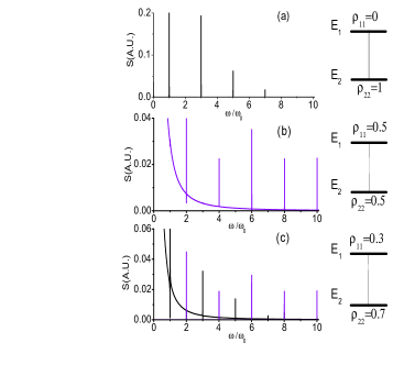
Figure 1: Emission spectra in double dots with different initial conditions. $\Delta=E_{1}-E_{2}=0.02$, $G_{12}=17.0$, and $\Gamma=6.8\times 10^{-8}\omega_{0}$.

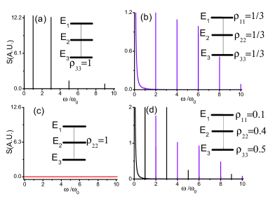
Figure 2: Emission spectra in triple dots for different initial conditions. The thin lines between the levels (in each dot) indicate the optical couplings between the dots with value $G=15.25$. $E_{1}-E_{2}=E_{2}-E_{3}=0.02$. $\Gamma=6.8\times 10^{-8}\omega_{0}$.

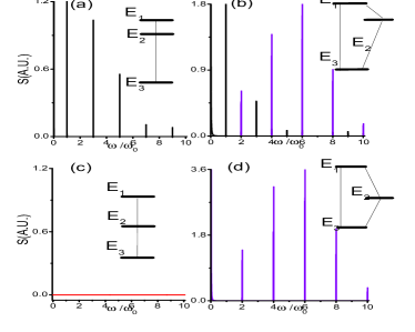
Figure 3: Emission spectra in triple dots with same initial condition $\rho_{22}=1.0$, but with different structures. The thin lines between the levels (in each dot) indicate the optical couplings between the dots with value $G=5.0$. (a) and (c) are the cases with chain structure. (b) and (d) are of loop structures. In (a) and (b), $E_{1}-E_{2}=0.01$, $E_{2}-E_{3}=0.02$; in (c) and (d) $E_{1}-E_{2}=E_{2}-E_{3}=0.02$. $\Gamma=6.8\times 10^{-8}\omega_{0}$.

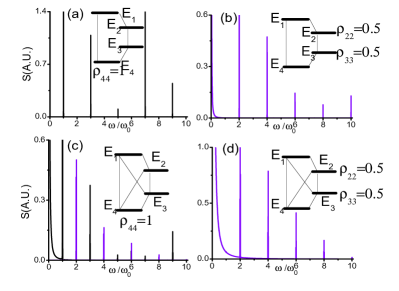
Figure 4: Emission spectra in quadruple dots with different structures/initial conditions. The thin lines between the levels (in each dot) indicate the optical couplings between the dots with value $G=6.3$. (a) and (b) are the cases with loop structure. (c) and (d) are of additional cross couplings. $E_{1}-E_{2}=E_{3}-E_{4}=0.008$, $E_{2}-E_{3}=0.02$. $\Gamma=6.8\times 10^{-8}\omega_{0}$.

Double dots We first consider the system of double dots with two levels. One can define Q as the time shift $\theta:t\rightarrow t+T/2$ combined with $\Omega_{1}:c_{1}\rightarrow-c_{1}$ (here and in the following $c_{j},j=1,...,N$, refers to the annihilation operator for state $|j\rangle$ in the dot j). It is easy to see that under such transformation H is invariant, $\hat{P}=G(c_{1}^{+}c_{2}+c_{2}^{+}c_{1})$ is odd, and the initial condition $\rho_{22}=1$ is invariant under transformation $\Omega_{1}$. So there is no even component and odd peaks appear only, as seen in Fig. (1a) and observed in many previous literatures. As our theory points out, the emission patterns depend on the initial condition. We can apply our theory with $\Omega_{2}:c_{1}\longleftrightarrow c_{2}$ for the initial condition $\rho_{11}=\rho_{22}=0.5$. In this case $\hat{P}$ is even. Thus there is no odd harmonic and only even harmonics appear as seen in Fig. (1b). (Note that these peaks may appear as very small split from exact even components.) It also agrees with our previous analytical perturbation results. It is a very striking fact that even the peak for $\omega_{0}$ (corresponding to Rayleigh peak, which is often very pronounced in the usual emission spectra) disappears due to the particular symmetry. As observed in Fig. (1c), there are both odd and even components for the initial condition $\rho_{11}=0.3,\rho_{22}=0.7$. This pattern is related to the fact that both symmetries $\Omega_{1}\cdot\theta$ and $\Omega_{2}\cdot\theta$ are broken.

Triple dots We first show we can use different initial conditions to realize quite different emission patterns. These results are displayed in Fig. 2. It is seen that the emission spectra may show odd only, even only, or both even and odd components. In particular, the emission may be completely quenched under appropriate condition. These results are based on our theorem. The symmetry property related to $\Omega_{1}:c_{2}\rightarrow-c_{2}$ leads to the disappearance of even harmonics in Fig. (2a). Symmetry $Q=\Omega_{2}\cdot\theta$, $\Omega_{2}:c_{1}\longleftrightarrow c_{3}$, results in the spectrum without odd harmonics shown in Fig. 2(b). Quite interestingly, both $\Omega_{1}$ and $\Omega_{2}$ are satisfied in Fig. (2c), which leads to the complete quenching of emission. This interesting phenomenon is a direct consequence of symmetry and is independent of the frequency of incident light. Thus it is different from the quenching of emission due to coherent trapping. The breaking of both symmetries $\Omega_{1}$ and $\Omega_{2}$ leads to emission with odd and even components as shown in Fig. (2d).

Figure 3 shows the dependence of emission patterns on the structure of nanosystems. Figs. (3a) and (3c) show systems with chain structures and Figs. (3b) and (3d) show systems with loop structures. Systems (c) and (d) are of symmetric energy levels, which is absent in systems (a) and (b). The different emission patterns are the direct consequences of the symmetries generated by $\Omega_{1}$ for (a), $\Omega_{2}$ for (d), $\Omega_{1}$ and $\Omega_{2}$ for (c) and none of $\Omega_{1}$ or $\Omega_{2}$ for (b).

Quadruple dots Our theorem is very powerful and can be applied to more general/complex nanostructures. Here we give one example of the tailoring the emission patters of quadruple dots. Careful design of structures of CQDs, or initial conditions leads to interesting emission spectra as shown in Fig. 4. The generators of the related symmetries are: $\Omega_{1}:c_{2}\rightarrow-c_{2},c_{4}\rightarrow-c_{4}$ for (4a); $\Omega_{2}:c_{2}\longleftrightarrow c_{3},c_{1}\longleftrightarrow c_{4}$ for (4b) and (4d); None for (4c).

Our theorem on the essential roles of symmetry for the emission patterns emphasizes the dynamic symmetry of the system, instead of spatial symmetry. For a system with spatial inversion symmetry $\Omega_{0}$, there may be odd harmonics only since the Hamiltonian is invariant under the symmetric operation $Q=\Omega_{0}\cdot\theta$ and $\hat{P}$ is odd under $\Omega_{0}$. It is clear that dynamic symmetry is more basic. Our theory points out that the emission spectra depend not only on Floquet states (in particular their parity), but also on the initial state. Moreover we’ve found nanostructures with more general symmetries, which lead to more interesting emission patterns. Our studies suggest the effective methods for generation the emission spectra with odd harmonics only, even harmonics only, both odd and even harmonics, or even quenching of all components. While previous work studied only the generation of even harmonics in addition to the odd harmonics (i.e. both odd and even harmonics appear). Our theory can be applied to more complex configurations.

We have considered the high-order harmonics generation from symmetry point of view. In experiments, the symmetric configuration could be realized by careful design the nanostructures. For instance, the energy levels can be adjusted by changing the confining potential. They could also be tuned by applying appropriate gate voltages. The optical couplings among the dots could be tuned by changing the inter-dot barriers, or the polarization of the incident field. In some situation, one may need weaker conditions. For instance, one may obtain the emission spectra with even harmonics only by using the configuration of triple-dot (loop structure) with degenerate levels for arbitrary inter-dot optical coupling. (It is a consequence of the symmetry generated by $Q=\Omega\cdot\theta$ with $\Omega$: $c_{i}\rightarrow-c_{i}$). Another issue is the preparation of the appropriate initial state. Some initial state, for example, that with electron staying in the lowest energy state, can be obtained easily. One may use some special designed laser pulse to prepare other types of initial states 9Bavli1993PRA . As also seen in section II, small derivation of the initial conditions may not change the picture. For instance, the main features of emission spectra remain unchanged if the derivation of occupation probability for the initial states is less than 5$\%$.

IV Summary

Based on the new theorem (on symmetry in the time domain and energy spectrum domain) we proved, we provide methods to tailor photon emission patterns in driven nanostructures by tuning the symmetry of the system. Apart from the emission spectra with only odd harmonics, or both odd and even harmonics, we are able to obtain emission spectra with just even harmonics. In suitable condition, the photon emission can even be fully quenched. Our methods for tailoring emission spectra apply for general coupled nanostructures.

V Acknowledgments

This work was partially supported by the National Science Foundation of China under Grants No.10874020, No. 10774016, and by the National Basic Research Program of China (973 Program) under Grants No. 2011CB922204. We thank Dr. N. Yang for helpful discussions.

References

- (1) K. J. Ahn, F. Milde, and A. Knorr, Phys. Rev. Lett. 98, 027401 (2007).
- (2) Y. Chassagneux, Nature (London) 457, 174 (2009).
- (3) S.Q. Duan, W. Zhang, Y. Xie, W.D. Chu,and X.G. Zhao, Phys. Rev. B 80, 1 (2009).
- (4) I. Baldea, Phys. Rev. B 69, 245311 (2004).
- (5) A. F. Terzis, and E. Paspalakis, Phys. Rev. B 80, 035307 (2009); J. Appl. Phys. 97, 023523 (2005).
- (6) V. Averbukh, O. E. Alon , and N. Moiseyev, Phys. Rev. A 64, 033411 (2001).
- (7) G. Ferrante, M. Zarcone, and S. A. Uryupin, Phys.Lett. A 335, 424 (2005).
- (8) H. P. Breuer, K. Dietz, and M. Holthaus, Z. Phys. D 8, 349 (1988); A. Peres, Phys. Rev. Lett. 67, 158 (1991); F. Grossmann, T. Dittrich, P. Jung, and P. Hanggi, Phys. Rev. Lett. 67, 516 (1991).
- (9) O. E. Alon, V. Averbukh, and N. Moiseyev, Phys. Rev. Lett. 80, 3743 (1998); Phys. Rev. Lett. 85, 5218 (2000); I. Baldea, A. K. Gupta, L. S. Cederbaum, and N. Moiseyev, Phys. Rev. B 69, 245311 (2004); N. Ben-Tal, N. Moiseyev, and A. Beswick, J. Phys. B 26, 3017(1993); H. M. Nilsen, L. B. Madsen, and J. P. Hansen, J. Phys. B 35, L403 (2002).
- (10) M. Xie, Phys. Res. A 483, 527 (2002).
- (11) G. Ferrante, M. Zarcone, and S. A. Uryupin, Phys. Lett. A 328, 481 (2004).
- (12) R. Bavli and H. Metiu, Phys. Rev. A 47, 3299 (1993).
- (13) T. Kreibich et al., Phys. Rev. Lett. 87, 103901 (2001).
- (14) P. P. Corso et al., J. Modern Opt. 54, 1387 (2007).
- (15) J. Wu, H. Qi and H. Zeng, Opt. lett. A 33, 2050 (2008).
- (16) Z. Zhou and J. Yuan, Phys.Rev.A 77, 063411 (2008).
- (17) J. Heslar et al., Int. J. Quantum Chem. 107,3159 (2007).
- (18) V. H. Le et al., Phys.Rev.A 76, 013414 (2007).
- (19) F. Quere et al., Phys.Rev.lett. 96, 125004 (2006).
- (20) A. McPherson et al., J. Opt. Soc. Am. B 4, 1753 (1987).
- (21) A. L. Huillier, K. J. Schafer, and K. C. Kulander, J. Phys. B 24, 3315 (1991).
- (22) M. Protopapas, C. H. Keitel, and P. L. Knight, Rep. Prog. Phys. 60, 389 (1997).
- (23) P. Sali res et al., Adv. At. Mol. Opt. Phys. 41, 83 (1999).
- (24) Z. Chang et al., Phys. Rev. Lett. 79, 2967(1997).
- (25) M. Schn rer et al., Phys. Rev. Lett. 80, 3236 (1998).
- (26) P. Sali res et al., Phys. Rev. Lett. 81, 5544 (1998).
- (27) P. P. Corso, L. L. Cascio, and F. Persico, Phys.Rev.A 58,1549 (1998).
- (28) L.M.Narducci et al., Phys.Rev.A 42, 1630 (1990).
- (29) M. L. Pons, R. Taieb, and A. Maquet, Phys. Rev. A 54, 3634 (1996); M. Frasca, Phys. Rev. A 60, 573 (1999); V. Delgado and J. M. G. Llorente, J. Phys. B 33, 5403 (2000).
- (30) H. Wang and X.G. Zhao, J. Phys.: Cond. Matt. 8, L285 (1996).