Simple Impurity Embedded in a Spherical Jellium:
Approximations of Density Functional Theory compared to
Quantum Monte Carlo Benchmarks

Abstract

We study the electronic structure of a spherical jellium in the presence of a central Gaussian impurity. We test how well the resulting inhomogeneity effects beyond spherical jellium are reproduced by several approximations of density functional theory (DFT). Four rungs of Perdew’s ladder of DFT functionals, namely local density approximation (LDA), generalized gradient approximation (GGA), meta-GGA and orbital-dependent hybrid functionals are compared against our quantum Monte Carlo (QMC) benchmarks. We identify several distinct transitions in the ground state of the system as the electronic occupation changes between delocalized and localized states. We examine the parameter space of realistic densities ($1\leq r_{s}\leq 5$) and moderate depths of the Gaussian impurity ($Z<7$). The selected 18 electron system (with closed-shell ground state) presents $1d\to 2s$ transitions while the 30 electron system (with open-shell ground state) exhibits $1f\to 2p$ transitions. For the former system, the accuracy for the transitions is clearly improving with increasing sophistication of functionals with meta-GGA and hybrid functionals having only small deviations from QMC. However, for the latter system, we find much larger differences for the underlying transitions between our pool of DFT functionals and QMC. We attribute this failure to treatment of the exact exchange within these functionals. Additionally, we amplify the inhomogeneity effects by creating the system with spherical shell which leads to even larger errors in DFT approximations.

I Introduction

Kohn–Sham density functional theory Hohenberg and Kohn (1964); Kohn and Sham (1965) (DFT) is now arguably the most popular computational method in theoretical condensed matter physics and materials science. While the method is exact in principle, in practice it is applied only with approximations to the unknown, exact exchange-correlation functional. The conventional semilocal approximations often fail to describe the structural, defect, and other properties of materials with strong electron-electron correlations—a failure that is not only quantitative but often qualitative. Indeed, even for less strongly correlated materials where the method yields reasonable predictions, further increases in accuracy are highly desired.

On the other hand, the quantum Monte Carlo (QMC) method allows direct solution of the many-body problem of interacting electrons using stochastic techniques Ceperley and Kalos (1979); Schmidt and Ceperley (1984); Hammond et al. (1994); Foulkes et al. (2001). In fact, the local density approximation is based on QMC calculations of the homogeneous electron gas Ceperley and Alder (1980) (HEG). The only significant source of systematic errors in the QMC method is the fixed-node approximation Anderson (1975); Reynolds et al. (1982) to the Fermion sign-problem. Using fixed-nodes, QMC has proven to been very effective in providing high accuracy results for many real systems such as molecules, clusters and solids with hundreds of valence electrons that are within 1-3% of experiment Foulkes et al. (2001); Grossman (2002); Nemec et al. (2010). More recently, new techniques have been developed to reduce the fixed-node errorsUmrigar et al. (2007); Reboredo et al. (2009); Bajdich et al. (2010), further improving the accuracy of the technique.

The spherical jellium system has been extensively investigated as a model of large clusters of simple metals (see, e.g., review [Brack, 1993]). It has been found to have pronounced shell structure with magic numbers $N=2,8,18,20,34,40,58,92,\ldots$ approximately corresponding to fully-filled closed shell of each orbital momentum as $1s^{2}|1p^{6}|1d^{10}|2s^{2}|1f^{14}|2p^{6}|1g^{18}|2d^{10}1h^{22}3s^{2}$. A few benchmark QMC studies exist Ballone et al. (1992); Harris and Ballone (1998); Sottile and Ballone (2001) for the total and correlation energies of closed-shells at magic numbers with up to 106 electrons. These results have been later compared against several DFT approximations Almeida et al. (2002); Tao et al. (2008). Surface correlation energies Sottile and Ballone (2001) and surface exchange-correlation energies Almeida et al. (2002); Tao et al. (2008) have been obtained using extrapolated values to infinite size. In general, the values obtained for correlation surface energies obtained with spheres are consistent with the latest DMC results for jellium slabs Wood et al. (2007) and other methods, but differ to some extent from the original DMC results from slab geometries Acioli and Ceperley (1996).

In this paper, we benchmark four levels of DFT approximations, following the “Jacob’s ladder” metaphor of Perdew and co-workers Perdew and Schmidt (2001); Tao et al. (2003); Perdew et al. (2005), by performing accurate quantum Monte Carlo calculations on the model of the interacting electron gas subject to a central impurity potential. The interacting electron gas is interpreted as a finite jellium sphere with $N$ electrons of average density $r_{s}$. An attractive spherical Gaussian of tunable strength at the origin represents the impurity potential. The proposed system closely relates to an atom in a real material while retaining a simplicity that is amenable to highly accurate solution under a wide range of conditions (slowly- and rapidly-varying density regions as well as a wide range of density values). The purpose of solving this simple model is to understand the role of electronic correlations and exchange, to understand the features that more sophisticated functional must possess in order to describe, e.g., strongly correlated materials, and to provide essentially exact benchmarks for testing new DFT approximations. Tabulated data of our results is given in Electronic Physics Auxiliary Publication Service (EPAPS) Document No. [].

II Models with Spherical Symmetry

II.1 Spherical Jellium Model

One of the simplest ways to neutralize the negative charge of $N$ electrons is to consider a sphere of positive charge $\rho_{B}$ of uniform density

$$\rho_{B}(r)=\left\{\begin{array}[]{ll}\frac{3}{4\pi}r_{s}^{-3},&r\leq R_{c}\equiv r_{s}N^{1/3}\\ 0,&r>R_{c},\end{array}\right.$$ (3)

with $r_{s}$ as adjustable parameter corresponding to a Wigner–Seitz radius in solids and $R_{c}$ as the sphere radius. This is a basic description of the spherical jellium model. The external potential due to the positive background is then

$$V_{ext}^{N}(r)=\left\{\begin{array}[]{ll}-\frac{1}{2}\frac{N}{R_{c}}\left(3-\frac{r^{2}}{R_{c}^{2}}\right),&r\leq R_{c}\\ -\frac{N}{r},&r>R_{c}.\end{array}\right.$$ (6)

The Hamiltonian of the electronic system (in atomic units) has the form

$${\mathcal{H}}=-\frac{1}{2}\sum_{i}^{N}\nabla^{2}_{i}+\sum_{i}^{N}V_{ext}^{N}(r_{i})+\frac{1}{2}\sum_{i,j\neq i}^{N}\frac{1}{|{\bf r}_{i}-{\bf r}_{j}|}+E_{self},$$ (7)

where we have introduced the constant Coulomb self energy of the positive background as

$$E_{self}=\frac{3}{5}\frac{N^{5/3}}{r_{s}}.$$ (8)

The addition of $E_{self}$ ensures that in the thermodynamic limit the energy of jellium spheres approaches the energy of HEG.

II.2 Spherical Jellium Model with a Gaussian Impurity

In order to further enhance the inhomogeneity effects in the jellium spheres, we propose the addition of the attractive Gaussian shaped impurity at the origin. The external potential is then modified as

$$V_{ext}^{N}(r)=-Z\exp(-r^{2}/\sigma^{2})+\left\{\begin{array}[]{ll}-\frac{1}{2}\frac{N}{R_{c}}\left(3-\frac{r^{2}}{R_{c}^{2}}\right),&r\leq R_{c}\\ -\frac{N}{r},&r>R_{c}\end{array}\right.$$ (11)

where $Z$ and $\sigma$ represent the depth and the width of the added Gaussian. The Gaussian form for the impurity is not meant to exactly describe core levels of a real atom, but to create additional localization for valence electrons. Moreover, using this model, we can also avoid the locality approximation required to evaluate conventional pseudopotentials Mitáš et al. (1991). As a welcome consequence, the Gaussian potential also preserves the cusp-less property of single-particle orbitals at the origin. To summarize, by controlling the amount of localization at the impurity, we can alter the shape and occupation order of single-particle states. We note that a similar potential has been used in studies of hetero-atomic clusters of Refs. Zhang et al., 1987; Baladron and Alonso, 1988.

II.3 Spherical Jellium Shell with a Gaussian Impurity

Another possibility to further amplify the inhomogeneity effects in the jellium is to create a spherical jellium shell. This can be achieved by combining external potentials [Eq. (6)] of a larger system with $N+M$ electrons and smaller system with $M$ electrons to form

$$V_{shell}^{N}(r)=V_{ext}^{N+M}(r)-V_{ext}^{M}(r)-Z\exp(-r^{2}/\sigma^{2}),$$ (12)

where integer variable $M\leq N$ controls the geometry of a shell [inner radius $R_{c}^{M}=r_{s}M^{1/3}$ and outer radius $R_{c}^{M+N}=r_{s}(M+N)^{1/3}$]. Note that in Eq. (12) the Gaussian impurity at the origin is also explicitly included. Above external potential closely resembles the potential of hollow clusters Pavlyukh and Berakdar (2010); Polozkov et al. (2009). The difference in our model is the addition of Gaussian impurity which attracts electron density towards the origin. In turn, the enhanced inhomogeneity (i.e., charge separation between center and shell) provides even more severe test for the single-particle methods studied here.

III Methods

The goal of this paper is to compare the total energies and radial densities of equivalent states of the spherical jellium systems in Hartree–Fock (HF), DFT and quantum Monte Carlo Methods. Due to the spherical symmetry of the system and because the spin-orbit interaction is not considered, the eigenstates of ${\mathcal{H}}$ must also be eigenstates of the angular momentum operators $L^{2}$ and $M_{L}$, spin operators $S^{2}$ and $M_{S}$. The advantage of the spherical symmetry is that rigorous upper-bound theorems apply for QMC and ground state DFT can be generalizedGunnarsson and Lundqvist (1976) for the lowest energy state states of each value of $L$ and $S$. Therefore, meaningful phase diagrams can be constructed with each method.

III.1 Criteria used to select eigenstates of $L$ and $S$

For benchmark purposes, we only need to compare equivalent states with DFT and QMC. For comparison, we have selected states that are likely but not guaranteed to be the minimum energy configurations. Since we are concerned with jellium densities of $1\leq r_{s}\leq 5$, our system can be characterized as weakly interacting. In this regime it is a reasonable to assume that, in analogy with atoms and 3D quantum dots Vorrath and Blümel (2003), the filling of the orbitals within a single shell of spherical jellium follows Hund’s rules, i.e., for a given electron configuration, the state with maximum multiplicity ($2S+1$) has the lowest energy, and for a given multiplicity, the state with the largest value of $L$ is likely to have the lowest energy. It is straightforward to construct the eigenfunction of ${}^{2S+1}L$ symmetry (in the Russell–Saunders term symbol notation) as the Slater determinant of single-particle orbitals with occupancies chosen such that $M_{L}\equiv\sum_{i}m_{i}=L$ and $M_{S}\equiv\sum_{i}s_{i}=S$. For $M_{L}\neq 0$, the determinants will be complex-valued, an issue important in the QMC context and discussed further bellow.

The original second Hund’s rule only applies to $3D$ spherically-symmetric systems, since it involves the total angular momentum $L$. There is debate, however, on the existence and form of a second Hund’s rule, with redefined shells, in the case of parabolic models of quantum dots in $2D$ at the highly correlated limit (see, e.g., Refs. Ghosal et al., 2007; Pederiva et al., 2000). While that debate is interesting, it is beyond the scope of this paper to validate the Hund’s rules in the range of parameters explored with our $3D$ models.

III.2 Single-particle Methods

To obtain the quantities of interest within single-particle methods we employ a non-relativistic atomic solver, originally implemented in Ref. [Vincent, 2006] and currently part of the QMCPACK suite Kim et al. , modified to handle pure HF method, LDA, GGA, meta-GGA and hybrid functionals. The single-particle orbitals are conveniently expressed as radial-functions $R_{n,l}(r)$ multiplied by an angular-part given as a spherical harmonic $Y_{l,m}(\theta,\phi)$. This choice ensures well defined quantum numbers.

The radial equations [$R_{n,l}(r)$] are iteratively solved via Numerov algorithm on a large logarithmic grid ($\sim$ 5000 points) until the tight convergence criteria are met ($\Delta E_{tot}<10^{-7}$ and $\Delta E_{eig}<10^{-14}$). For the later cases of the open shells we use the spin-unrestricted formulation of the HF and DFT theories. In short, in our formulation, we perform the spin-dependent average of the effective potentials within each sub-shell of the same $n$ and $l$, resulting in a single radial function. As we discuss in the next subsection, these radial functions are then directly imported into QMC methods.

In general, the Kohn–Sham and HF wave functions have a form of a single Slater determinant and are explicit eigenstates of $M_{S}$, but they are eigenstates of $S^{2}$ only if $|M_{S}|$ has the maximum value. Therefore, the $L$ and $S$ eigenstates with maximum multiplicity ($2S+1$) and with the largest value of $L$ automatically have the correct spin symmetry.

In order to simplify the DFT implementation, for open shell cases, we have neglected the angular dependence of the spin-densities for calculation of the exchange-correlation. This treatment is commonly known as the spherical approximation used in many DFT atomic solvers for production of pseudopotentials. A very good numerical agreement (better than 1 mHa) was achieved between our and other atomic solvers (OPIUM Walter , FHI98PP M. Fuchs (1999) and APE Oliveira and Nogueira (2008)) for several open and closed shell atomic states and functionals. The four rungs of Perdew’s ladder of approximate DFT functionals are represented by the Perdew–Wang (PW) LDA Perdew and Wang (1992), Perdew–Burke–Ernzerhof (PBE) GGA Perdew et al. (1996), Tao–Perdew–Staroverov–Scuseria (TPSS) meta-GGA Tao et al. (2003) and PBE hybrid (PBE0) Ernzerhof and Scuseria (1999) exchange-correlation functionals as implemented in the LIBXC library Marques and in the Quantum Espresso suite et. al. .

III.3 Quantum Monte Carlo Methods

The trial many-body wave function serves as the most important input for the quantum Monte Carlo methods within the fixed-node diffusion Monte Carlo approach. For this problem, following the approach used in previous studies Ballone et al. (1992); Harris and Ballone (1998); Sottile and Ballone (2001), we choose a many-body wavefunction that is a product of spin-up and spin-down Slater determinants ($D$) and a Jastrow correlation factor ($J$), written as

$$\Psi_{T}({\bf r}_{1},{\bf r}_{2},\ldots,{\bf r}_{N})= D[\varphi^{\uparrow}_{1}({\bf r}_{1}),\ldots,\varphi^{\uparrow}_{M}({\bf r}_{M})]$$

$$\times D[\varphi^{\downarrow}_{1}({\bf r}_{M+1}),\ldots,\varphi^{\downarrow}_{N-M}({\bf r}_{N})]$$

$$\times\exp[J({\bf r}_{1},{\bf r}_{2},\ldots,{\bf r}_{N})],$$ (13)

assuming the first $M$ electrons to be spin-up and the remaining $N-M$ to be spin-down. The Slater determinants are constructed from orbitals generated in single-particle methods and have a form

$$\varphi^{\uparrow(\downarrow)}_{k=n,l,m}({\bf r}_{i})=R^{\uparrow(\downarrow)}_{n,l}(r_{i})Y_{l,m}(\theta_{i},\phi_{i}).$$ (14)

The symmetric Jastrow correlation factor includes well-known electron-electron cusp conditions as well as one and two-body correlation functions (for details see, e.g., Ref. [Bajdich, 2007]). As a note, we did not find it necessary to include the multipolar terms into the Jastrow factor as in Ref. Sottile and Ballone, 2001.

The Jastrow term is further variationally optimized Umrigar and Filippi (2005); Umrigar et al. (2007). The optimal $\Psi_{T}$ is then used in diffusion Monte Carlo (DMC) method to obtain the ground state fixed-node (FN) energies and other expectation values of the system. As a additional step, for selected states, we also perform reptation Monte Carlo (RMC) calculations Baroni and Moroni (1999) to obtain pure expectation values of the fixed-node densities. All the QMC calculations were performed using QWalk code Wagner et al. (2009).

As we have already mentioned, the $L$ and $S$ eigenfunctions considered in this paper with $M_{L}\neq 0$ are complex-valued and require the use of the fixed-phase DMC algorithmOrtiz et al. (1993). However, the associated fixed-phase errors are in general different (and possibly larger) than the fixed-node errors for real-valued wavefunctionsReboredo (2010). To avoid mixing results with two different approximations, we exclusively use the real-valued $M_{L}=0$ projections of the same $LS$ eigenfunction (as they are energetically degenerate). The $M_{L}=0$ projections can be readily obtained from $M_{L}=L$ states by the recursive application of the momentum lowering $L^{-}$ operator. As a consequence, the complex-valued single Slater determinant is replaced by the real-valued linear combination of Slater determinants. Please refer to the Appendix for the linear combinations used for each open shell state.

IV Results

IV.1 Tests and validations

To test the numerical implementation of our HF, DFT and fixed-node (FN) DMC methods we have recalculated previous results for the closed-shell jellium spheres. We achieve an excellent agreement with the PW LDA and PBE GGA energies of Ref. Almeida et al., 2002 and with TPSS meta-GGA energies of Ref. Tao et al., 2008. Obtained results for HF energies are identical to Ref. Madjet et al., 1995 for model sodium clusters of $r_{s}=4.0$ with up to 196 electrons. However, we find lower HF energies (by $0.5$ mHa per electron) when compared to energies of Ref. Sottile and Ballone, 2001. This is most likely due to the non-self consistent treatment of HF in Ref. Sottile and Ballone, 2001. Finally, all our FN-DMC energies using LDA orbitals are within error-bars of FN-DMC energies of the Ref. Sottile and Ballone, 2001. The sole exception is the 2 electron system at $r_{s}=1$, where the differences are larger.

The single limitation for the DMC calculations comes from the use of fixed-node approximation. Introduced fixed-node errors can be reduced by expanding the trial wave function in multi-determinants Umrigar et al. (2007); Bajdich et al. (2010) or by using the backflow correlation corrections Feynman and Cohen (1956); Kwon et al. (1998); López Ríos et al. (2006); Bajdich et al. (2008), or both. Previously, it was found that the QMC calculations for the closed shell jellium spheresSottile and Ballone (2001) did not suffer from large fixed-node errors (by comparing to FN-DMC results with small multi-determinant expansions Harris and Ballone (1998)). In order to systematically check for these errors, we have extended the previous FN-DMC calculations to include backflow correlations for all the densities and particle numbers. We find small and uniform gains to correlation energies on the order of 0.3 mHa per electron. Therefore, it is very reasonable to assume that, for the energy differences considered here, these small corrections cancel out.

IV.2 Results for the spherical jellium with impurity

IV.2.1 $1d\to 2s$ transitions for N=18

The excellent agreement for the closed-shell energies of jellium spheres, obtained with both with QMC and DFT methods, with earlier publications gives us confidence to study open shells. As the first testing case, we have selected a jellium sphere with 18 electrons, which for the impurity free system is one of the fully-filled closed shells and corresponds to a cluster with a stable configuration. As we increase the attractive Gaussian potential of the impurity, the nearest unoccupied $2s$ level is lowered in energy below the $1d$ level. Interestingly, exactly the same crossing of the levels was previously observed in the context of hetero-atomic clusters Zhang et al. (1987); Baladron and Alonso (1988) and 3D quantum dots Vorrath and Blümel (2003). As a result, the ground state of the system will change from closed shell occupation ${}^{1}S(1s^{2}1p^{6}1d^{10})$ to either ${}^{3}D(1s^{2}1p^{6}1d^{9}2s^{1})$ or ${}^{3}F(1s^{2}1p^{6}1d^{8}2s^{2})$ open shell occupations. As a note, each state differs in occupation in more than one shell ($1d$ and $2s$) while Hund’s rules strictly apply only to occupations within a single shell.

The phase diagram depends on the variables $r_{s}$, $Z$ and $\sigma$. We limit our discussion to realistic density range between $r_{s}=1$ and $r_{s}=5$ found in the majority of bulk systems. Since the $\sigma$ and $Z$ parameters are effectively coupled together, we choose to fix the width of the Gaussian at $\sigma=0.6$ and vary only its depth $Z$. As a result, we find robust $1d\to 2s$ transitions within $0<Z<7$. We summarize our calculations in the phase diagram, Fig. 1.

There are several general observations which can be drawn from the phase diagram, Fig. 1. As we increase the attractiveness of the impurity, we see changes on the occupation of a more delocalized $1d$ orbital to more localized atomic-like $2s$ orbital in the following order: $1d^{10}\to 1d^{9}2s^{1}\to 1d^{8}2s^{2}$. In addition, we notice the existence of high density region ($r_{s}<1.4$) which has always partial $2s$ occupation (see also Table 1). This region for jellium spheres at $r_{s}=1$ was not discussed in previous studies.

Table 1: Comparison between the total energies of the closed-shell ${}^{1}S$ and open-shell ${}^{3}F$ states for $N=18$ and $r_{s}=1$. The latter state is clearly lower in energy.

state	EDMC	ELDA	EPBE	EHF
${}^{1}S$	0.39104(2)	0.39317	0.38908	0.42786
${}^{3}F$	0.38817(2)	0.39030	0.38628	0.42386

From a methodological point of view, Fig. 1 provides detailed comparison between the single-particle methods and our DMC benchmarks. Our first observation is that HF greatly overestimates while LDA underestimates the region of the stability of the ${}^{3}D(1s^{2}1p^{6}1d^{9}2s^{1})$ state. In fact LDA and HF bracket our best estimate, which is not surprising considering the success of hybrid functionals. Second, the GGA rung of the functional ladder represented by the PBE leads to clear improvement in accuracy over LDA. Next, the TPSS meta-GGA and PBE0 hybrid functionals agree even closer with DMC predictions than PBE however without particular order in accuracy.

Last, to give some measure of the fixed-node errors, we also compare the DMC results using LDA orbitals with DMC results using HF orbitals. Despite the different nodes resulting from these choices the DMC energies are very similar indicating that the nodal errors remain small.

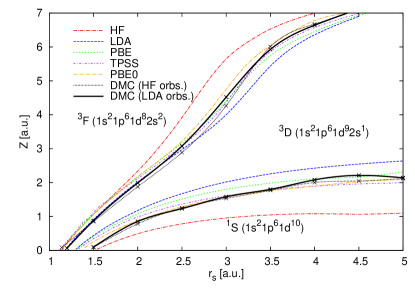
Figure 1: Phase diagram of spherical jellium with 18 electrons and for fixed $\sigma=0.6$ as a function of density $r_{s}$ and impurity potential strength $Z$. The transitions between the three lowest lying states are shown for unrestricted Hartree–Fock (HF) (red dot-dashed), PW LDA (blue dashed), PBE GGA (green short-dashed), TPSS meta-GGA (purple dot-dashed), PBE0 hybrid (orange dot-dashed), DMC with UHF orbitals (black dot-dashed) and DMC with LDA orbitals (black full) lines (see also text). The lines in the figure are extrapolations over the discrete points by cubic splines.

IV.2.2 $1f\to 2p$ transitions for N=30

In general, the behavior of the 30 electron system with a partially-occupied $1f$ shell is similar to the case with 18 electrons. The main difference is that, for the impurity free system, the ground state configuration is characterized by a high-spin quintet state at $1f$ shell and with $2p$ as the closest empty level. Therefore, the role of the extended orbital that transfers the electron is taken by $1f$ while $1p$ localizes and receives an electron as the impurity potential is applied.

Since $1p$ is more degenerate than $1s$, the 30 electron systems allows us to study more complicated effects of correlations and exchange at the impurity as we change the impurity potential. The accessible states of the interest are ${}^{5}I(1s^{2}1p^{6}1d^{10}2s^{2}1f^{10})$, ${}^{7}I(1s^{2}1p^{6}1d^{10}2s^{2}1f^{9}2p^{1})$, ${}^{9}G(1s^{2}1p^{6}1d^{10}2s^{2}1f^{8}2p^{2})$ and ${}^{11}S(1s^{2}1p^{6}1d^{10}2s^{2}1f^{7}2p^{3})$.

In Fig. 2 we directly compare the phase diagram obtained with DMC and mean field methods used in the 18 electron case. The detailed comparison shown in Fig. 2 reveals several important features. First, LDA, PBE GGA and TPSS meta-GGA, all semilocal functionals, predict almost identical boundaries. When compared with our DMC results, we find that only the locations of ${}^{5}I\leftrightarrow^{11}S$ and ${}^{5}I\leftrightarrow^{7}I$ phase transitions agree well, while the ${}^{7}I\leftrightarrow^{9}G$ and ${}^{9}G\leftrightarrow^{11}S$ transitions are shifted to lower $Z$ values. Second, PBE0 hybrid corrects slightly for the lower $Z$ shifts in the ${}^{7}I\leftrightarrow^{9}G$ and ${}^{9}G\leftrightarrow^{11}S$ transitions. In contrast, HF method produces much more satisfactory agreement with DMC for smaller densities ($r_{s}>2.5$) but greatly overestimates the stability of ${}^{11}S$ state at higher densities ($r_{s}<2.2$) due to the missing correlation. The behavior described above suggest that a) the inhomogeneity effects in the density are relatively small and well captured by the semilocal functionals; b) the full non-local exchange absent at the semilocal level and only partially present (25%) in PBE0 functional is needed to correct for lower $Z$ shifts.

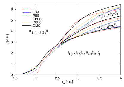
Figure 2: Phase space diagram for jellium with 30 electrons and for fixed $\sigma=1.5$ as a function of density $r_{s}$ and impurity strength $Z$. We have identified ${}^{5}I$, ${}^{7}I$, ${}^{9}G$ and ${}^{11}S$ states as occupying this section of the $r_{s}$-$Z$ space. The convention for lines is identical to Fig. 1.

IV.3 Results for the spherical jellium shell with impurity

IV.3.1 $1d\to 2s$ transitions for N=18

As in the first case of the spherical jellium with impurity, we choose to study the 18 electron system in the spherical shell potential [Eq. (12)]. The occupation of the single-particle states for hollow cluster is assumed to be the same as for jellium spheres (as confirmed by Ref. Polozkov et al., 2009). Rather than finding the extensive phase space diagram of the system we limit our study to a very small subset of the space. We select $M=9$, $r_{s}=3.0$ and $Z\sim 8.5$ to illustrate a size of localization errors from HF and DFT based theories.

Figure 3 compares the energy difference between ${}^{3}D$ and ${}^{3}F$ states as a function of $Z$ calculated with single-particle methods and DMC. Arguably, the main point of interest in Fig. 3 is the slope around ${}^{3}D\leftrightarrow^{3}F$ transition and secondly the size of the relative errors. As in previous subsection, all semilocal functionals (i.e., LDA, PBE, TPSS) results have a very similar slope (with half the steepness of the DMC curve). On the other hand, the slope of the HF curve is almost identical to DMC curve. Not surprisingly, PBE0 partially recovers the correct slope as it contains 25% of exact exchange.

Finally, it is also instructive to analyze the radial densities for the ${}^{3}D$ and ${}^{3}F$ states (see Fig. 4). As a benchmark we use the pure expectation of the density operator from reptation Monte Carlo Baroni and Moroni (1999)(RMC) method with LDA orbitals. The densities for each state and spin channel in Fig. 4 have a distinct double peak structure – the smallest is due to the presence of the Gaussian impurity and the largest due to the spherical shell itself. Also visible is the relative reduction of the smaller peak for the ${}^{3}D$ spin-down channel due to the absence of the more localized $2s$ state.

From the direct comparison with RMC results we deduce that the density at inner shell regions (i.e., smaller peak) is better described within HF while LDA and PBE GGA provide better densities for the outer shell regions (i.e., larger peak). The PBE0 hybrid smoothly interpolates between PBE and HF limits with the best overall description. Lastly, the TPSS meta-GGA results in an substantial increase of density at both peaks and decrease at the tails when compared to LDA and PBE GGA. We find this overcompensation of the density, presumably due to the kinetic energy density contributions specific to the TPSS functional, to be surprisingly high.

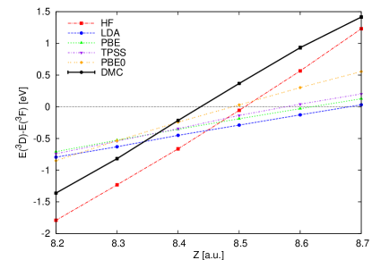
Figure 3: Total energy difference between ${}^{3}D$ and ${}^{3}F$ states of the spherical jellium shell of 18 electrons with $M=9$, $r_{s}=3.0$ and $\sigma=0.6$ in a small window of $Z$. All the methods are described in the text.

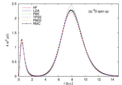
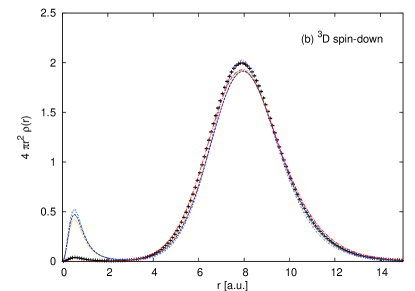
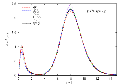
Figure 4: Radial densities for the spherical jellium shell of 18 electrons for ${}^{3}D$ (upper) ${}^{3}F$ (lower) states with $M=9$, $r_{s}=3.0$, $Z=8.5$ and $\sigma=0.6$. Spin-up channel (left figure) and spin-down channel (right figure). All the methods are mentioned in the text and the convention for lines is identical to Fig. 1. The pure expectation of the density operator from RMC method employed LDA orbitals.

V Summary

In conclusion, we have studied the performance of a variety of DFT functionals with increasing complexity against quantum Monte Carlo benchmark in a spherical jellium model and an spherical shell model with an attractive Gaussian impurity at the center. The tunable strength of the impurity allowed us to find a number of interesting transitions between closed and open shell states. Our results shows that the development of better density functional approximation is increasingly required as the system departs from the perfect spherical jellium case. We report several regions where the employed approximations of DFT fail to find the same ground state as identified with QMC methods.

The $1d\to 2s$ transitions in 18 electron system are well described on the highest semilocal level (TPSS meta-GGA) as well in global hybrid (PBE0) DFT. On the other hand, not all $1f\to 2p$ transitions in the 30 electron system were accurately captured. We argue that even as the inhomogeneity effects in the density are relatively small and well captured by the semilocal functionals, full non-local exchange is needed to accurately describe the system. Our work therefore further supports the need for the hyper-GGA functionals Perdew et al. (2008) with fully non-local exchange and accompanying balanced correlation.

In the spherical jellium-shell model with an impurity at the center, where the inhomogeneity in the electronic density is increased, the DFT methods with exact-exchange give better agreement for the studied transitions. The radial electron densities in the inner region closest to the impurity are correctly described at the HF level, while LDA and PBE GGA are more accurate in the outer region. The PBE0 global-hybrid results smoothly interpolates between HF and GGA. We find surprisingly high deviations in density for the TPSS. Finally, we also publish our results in the EPAPS Document No. [] with the purpose of allowing a detailed comparison with newly developed DFT functionals.

Appendix: Real-valued $LS$ eigenfunctions

Application of $(L^{-})^{L}$ operator on the $LS$ eigenfunction with $M_{L}=L$ leads to real-valued $LS$ eigenfunction with $M_{L}=0$. The linear combinations of Slater determinants for the open-shell states in 18 electron system are then

$$\Psi[^{3}D(1d^{4\downarrow})]= D_{1}$$ (15)

$$\Psi[^{3}F(1d^{3\downarrow})]= \frac{1}{\sqrt{5}}(D_{2}+2D_{3}),$$ (16)

where $D_{1}=(2^{-},1^{-},-1^{-},-2^{-})$, $D_{2}=(1^{-},0^{-},-1^{-})$ and $D_{3}=(2^{-},0^{-},-2^{-})$ are determinants with indicated relevant occupied orbitals (numbers stand for the orbital quantum numbers and superscripts indicate the spins).

The $M_{L}=0$ linear combinations for the 30 electron system are

$$\Psi[^{9}G(1f^{\downarrow}2p^{2\uparrow})]= \frac{1}{\sqrt{7}}\left[\sqrt{2}(D_{1}+D_{2})+\sqrt{3}D_{3}\right],$$ (17)

where $D_{1}=(-1^{-},1^{+},0^{+})$, $D_{2}=(1^{-},0^{+},-1^{+})$, $D_{3}=(0^{-},1^{+},-1^{+})$ and

$$\Psi[^{7}I(1f^{2\downarrow}2p^{\uparrow})]= \frac{1}{6\sqrt{7}\sqrt{11}}[30D_{4}+24D_{5}+6D_{6}$$

$$+5\sqrt{6}D_{7}+9\sqrt{5}D_{8}+5\sqrt{3}D_{9}$$

$$+5\sqrt{6}D_{10}+9\sqrt{5}D_{11}+5\sqrt{3}D_{12}],$$ (18)

where $D_{4}=(1^{-},-1^{-},0^{+})$, $D_{5}=(2^{-},-2^{-},0^{+})$, $D_{6}=(3^{-},-3^{-},0^{+})$, $D_{7}=(0^{-},-1^{-},1^{+})$, $D_{8}=(1^{-},-2^{-},1^{+})$, $D_{9}=(2^{-},-3^{-},1^{+})$, $D_{10}=(1^{-},0^{-},-1^{+})$, $D_{11}=(2^{-},-1^{-},-1^{+})$, $D_{12}=(3^{-},-2^{-},-1^{+})$ and

$$\Psi[^{5}I(1f^{3\downarrow})]= \frac{1}{\sqrt{2}\sqrt{3}\sqrt{7}\sqrt{11}}[5D_{13}+16D_{14}+9D_{15}$$

$$+5\sqrt{2}(D_{16}+D_{17})],$$ (19)

where $D_{13}=(1^{-},0^{-},-1^{-})$, $D_{14}=(2^{-},0^{-},-2^{-})$, $D_{15}=(3^{-},0^{-},-3^{-})$, $D_{16}=(2^{-},1^{-},-3^{-})$,$D_{17}=(3^{-},-1^{-},-2^{-})$. Above results have been also verified numerically using code from Ref. Zhuang and C, 2009.

References

- Hohenberg and Kohn (1964) P. Hohenberg and W. Kohn, Phys. Rev. 136, B864 (1964).
- Kohn and Sham (1965) W. Kohn and L. J. Sham, Phys. Rev. 140, A1133 (1965).
- Ceperley and Kalos (1979) D. M. Ceperley and M. H. Kalos, in Monte Carlo Methods in Statistical Physics, edited by K. Binger (Springer, Berlin, 1979), pp. 145–194.
- Schmidt and Ceperley (1984) K. E. Schmidt and D. M. Ceperley, in Monte Carlo Methods in Statistical Physics 2, edited by K. Binger (Springer, Berlin, 1984), pp. 279–355.
- Hammond et al. (1994) B. L. Hammond, W. A. Lester Jr., and P. J. Reynolds, Monte Carlo Methods in ab initio quantum chemistry (World Scientific, Singapore, 1994).
- Foulkes et al. (2001) W. M. C. Foulkes, L. Mitas, R. J. Needs, and G. Rajagopal, Rev. Mod. Phys. 73, 33 (2001).
- Ceperley and Alder (1980) D. M. Ceperley and B. J. Alder, Phys. Rev. Lett. 45, 566 (1980).
- Anderson (1975) J. B. Anderson, J. Chem. Phys. 63, 1499 (1975).
- Reynolds et al. (1982) P. J. Reynolds, D. M. Ceperley, B. J. Alder, and W. A. Lester, J. Chem. Phys. 77, 5593 (1982).
- Grossman (2002) J. Grossman, J Chem. Phys. 117, 1434 (2002).
- Nemec et al. (2010) N. Nemec, M. D. Towler, and R. J. Needs, J Chem. Phys. 132, 034111 (pages 7) (2010).
- Umrigar et al. (2007) C. J. Umrigar, J. Toulouse, C. Filippi, S. Sorella, and R. G. Hennig, Phys. Rev. Lett. 98, 110201 (2007).
- Reboredo et al. (2009) F. A. Reboredo, R. Q. Hood, and P. R. C. Kent, Phys. Rev. B 79, 195117 (2009).
- Bajdich et al. (2010) M. Bajdich, M. L. Tiago, R. Q. Hood, P. R. C. Kent, and F. A. Reboredo, Phys. Rev. Lett. 104, 193001 (2010).
- Brack (1993) M. Brack, Rev. Mod. Phys. 65, 677 (1993).
- Ballone et al. (1992) P. Ballone, C. J. Umrigar, and P. Delaly, Phys. Rev. B 45, 6293 (1992).
- Harris and Ballone (1998) M. Harris and P. Ballone, Solid State Commun. 105, 725 (1998).
- Sottile and Ballone (2001) F. Sottile and P. Ballone, Phys. Rev. B 64, 045105 (2001).
- Almeida et al. (2002) L. M. Almeida, J. P. Perdew, and C. Fiolhais, Phys. Rev. B 66, 075115 (2002).
- Tao et al. (2008) J. Tao, J. P. Perdew, L. M. Almeida, C. Fiolhais, and S. Kümmel, Phys. Rev. B 77, 245107 (2008).
- Wood et al. (2007) B. Wood, N. D. M. Hine, W. M. C. Foulkes, and P. García-González, Phys. Rev. B 76, 035403 (2007).
- Acioli and Ceperley (1996) P. H. Acioli and D. M. Ceperley, Phys. Rev. B 54, 17199 (1996).
- Perdew and Schmidt (2001) J. P. Perdew and K. Schmidt, in Density Functional Theory and Its Application to Materials, edited by P. G. V. Van Doren, C. Van Alsenoy (AIP, Melville, NY, 2001), pp. 1–20.
- Tao et al. (2003) J. Tao, J. P. Perdew, V. N. Staroverov, and G. E. Scuseria, Phys. Rev. Lett. 91, 146401 (2003).
- Perdew et al. (2005) J. P. Perdew, A. Ruzsinszky, J. Tao, V. N. Staroverov, G. E. Scuseria, and G. I. Csonka, J. Chem. Phys. 123, 062201 (2005), ISSN 00219606.
- Mitáš et al. (1991) L. Mitáš, E. L. Shirley, and D. M. Ceperley, J. Chem. Phys. 95, 3467 (1991).
- Zhang et al. (1987) S. B. Zhang, M. L. Cohen, and M. Y. Chou, Phys. Rev. B 36, 3455 (1987).
- Baladron and Alonso (1988) C. Baladron and J. A. Alonso, Physica B: Cond. Matt. 154, 73 (1988).
- Pavlyukh and Berakdar (2010) Y. Pavlyukh and J. Berakdar, Phys. Rev. A 81, 042515 (2010).
- Polozkov et al. (2009) R. G. Polozkov, V. K. Ivanov, A. V. Verkhovtsev, and A. V. Solov’yov, Phys. Rev. A 79, 063203 (2009).
- Gunnarsson and Lundqvist (1976) O. Gunnarsson and B. I. Lundqvist, Phys. Rev. B 13, 4274 (1976).
- Vorrath and Blümel (2003) T. Vorrath and R. Blümel, Eur. Phys. J. B 32, 227 (2003).
- Ghosal et al. (2007) A. Ghosal, A. D. Güçlü, C. J. Umrigar, D. Ullmo, and H. U. Baranger, Phys. Rev. B 76, 085341 (2007).
- Pederiva et al. (2000) F. Pederiva, C. J. Umrigar, and E. Lipparini, Phys. Rev. B 62, 8120 (2000).
- Vincent (2006) J. E. Vincent, Ph.D. thesis, UIUC (2006).
- (36) J. Kim et al., QMCPACK simulation suite, URL http://qmcpack.cmscc.org.
- (37) E. J. Walter, OPIUM pseudopotential package, URL http://opium.sourceforge.net.
- M. Fuchs (1999) M. S. M. Fuchs, Comput. Phys. Commun. 119, 67 (1999).
- Oliveira and Nogueira (2008) M. Oliveira and F. Nogueira, Comput. Phys. Comm. 178 (2008).
- Perdew and Wang (1992) J. P. Perdew and Y. Wang, Phys. Rev. B 45, 13244 (1992).
- Perdew et al. (1996) J. P. Perdew, K. Burke, and M. Ernzerhof, Phys. Rev. Lett. 77, 3865 (1996).
- Ernzerhof and Scuseria (1999) M. Ernzerhof and G. E. Scuseria, J. Chem. Phys. 110, 5029 (1999).
- (43) M. A. L. Marques, LibXC library, URL http://www.tddft.org/programs/octopus/wiki/index.php/Libxc.
- (44) P. G. et. al., Quantum-Espresso package, URL http://www.quantum-espresso.org.
- Bajdich (2007) M. Bajdich, Ph.D. thesis, NCSU (2007).
- Umrigar and Filippi (2005) C. J. Umrigar and C. Filippi, Phys. Rev. Lett. 94, 150201 (2005).
- Baroni and Moroni (1999) S. Baroni and S. Moroni, Phys. Rev. Lett. 82, 4745 (1999).
- Wagner et al. (2009) L. K. Wagner, M. Bajdich, and L. Mitas, J. Comp. Phys. 228, 3390 (2009).
- Ortiz et al. (1993) G. Ortiz, D. M. Ceperley, and R. M. Martin, Phys. Rev. Lett. 71, 2777 (1993).
- Reboredo (2010) F. A. Reboredo, arXiv 1008, 0359 (2010), under review in Phys. Rev. B.
- Madjet et al. (1995) M. Madjet, C. Guet, and W. R. Johnson, Phys. Rev. A 51, 1327 (1995).
- Feynman and Cohen (1956) R. P. Feynman and M. Cohen, Phys. Rev. 102, 1189 (1956).
- Kwon et al. (1998) Y. Kwon, D. M. Ceperley, and R. M. Martin, Phys. Rev. B 58, 6800 (1998).
- López Ríos et al. (2006) P. López Ríos, A. Ma, N. D. Drummond, M. D. Towler, and R. J. Needs, Phys. Rev. E 74, 066701 (2006).
- Bajdich et al. (2008) M. Bajdich, L. Mitas, L. K. Wagner, and K. E. Schmidt, Phys. Rev. B 77, 115112 (2008).
- Perdew et al. (2008) J. P. Perdew, V. N. Staroverov, J. Tao, and G. E. Scuseria, Phys. Rev. A 78, 052513 (2008).
- Zhuang and C (2009) X. Zhuang and B. N. C, Chinese Phys. B 18, 542 (2009).