Model for projectile fragmentation: case study for Ni on Ta, Be and Xe on Al

Abstract

For projectile fragmentation we work out details of a model whose origin can be traced back to the Bevalac era. The model positions itself between the phenomenological EPAX parametrization and microscopic transport models like “Heavy Ion Phase Space Exploration Model”(HIPSE) and antisymmetrised molecular dynamics(AMD). We apply the model to some recent data of projectile fragmentation of Ni on Ta and Be at beam energy 140 MeV/nucleon and some older data of Xe on Al at beam energy 790 MeV/nucleon. Reasonable values of cross-sections for various composites populated in the reactions are obtained.

I Introduction

In heavy ion collisions, if the beam energy is high enough, the following scenario can be envisaged. For a general impact parameter, part of the projectile will overlap with part of the target. This is the participant region where violent collisions occur. In addition there are two mildly excited remnants: projectile like fragment (PLF), with rapidity close to that of the projectile rapidity and target like fragment (TLF) with rapidity near zero. The PLF has been studied experimentally, this being one of the tools for production and identification of exotic nuclei.

The PLF has mild excitation and breaks up into many composites. Extensive measurements of cross-sections of composites arising from the break up of PLF of Ni on Be and Ta were made at Michigan State UniversityMocko1 . Powerful and elaborate calculations for the case of Ni on Be were made recently using transport modelMocko2 . Unfortunately calculations for Ni on Ta could not be done because this becomes prohibitively large. One of the main reasons of this venture was to examine if an alternate, less ambitious but realistic model, could be used to calculate results for the case of Ni on Ta. It appears that above a certain beam energy the model will be in general applicable and is implementable.

Great progress has been made in phenomenological EPAX Summerer model which predicts results for cross-sections. Our model, we believe is less phenomenological. It is grounded in traditional concepts of heavy ion reaction plus by now, well-known model of multifragmentation. We describe the basics of the model below.

II Model Assumptions

Imagine that the beam energy is high enough so that using straight line trajectories one can uniquely define participant,PLF and TLF. A certain fraction of the projectile is lost in the participant. This can be calculated. What remains of the projectile is the PLF, moving with velocity close to the beam velocity. There is a probability of having N neutrons and Z protons in the PLF. This probability $P_{N,Z}(b)$ depends upon the impact parameter. We call this abrasion. The abrasion cross-section when there are $N$ neutrons and $Z$ protons in the PLF is labelled by $\sigma_{a,N,Z}$:

$$\sigma_{a,N,Z}=\int 2\pi bdbP_{N,Z}(b)$$ (1)

This is stage 1 of the calculation.

An abraded system with $N$ neutrons and $Z$ protons has excitation. We characterise this by a temperature $T$ instead. This will expand and break up into many excited composites and nucleons. This break up is calculated using a canonical thermodynamic model(CTM) Das . The cross-section at this stage is called $\sigma_{n,z}^{pr}$. This is the second stage of the calculation. This second stage can be replaced by another statistical multifragmentation model(SMM) Bondorf but the results are expected to be very similar Chaudhuri1 .

Lastly we consider composites after stage 2. These have a temperature and can evaporate light particles like neutrons, protons, alphas etc. This can deplete a nucleus with neutron and proton numbers $n$ and $z$ that was obtained after stage 2 but there is a compensation also by feeding from higher mass nuclei.

III Calculational Details

Consider the abraison stage. The projectile hits the target. Use straightline geometry. We can then calculate the volume of the projectile that goes into the participant region (eqs. A.4.4 and A.4.5 of Dasgupta1 ). What remains in the PLF is $V$. This is a function of $b$, the impact parameter. If the original volume of the projectile is $V_{0}$, the original number of neutrons is $N_{0}$ and the original number of protons is $Z_{0}$ then the average number of neutrons in the PLF is $<N(b)>=(V(b)/V_{0})N_{0}$ and the average number of protons is $<Z(b)>=(V(b)/V_{0})Z_{0}$. These will usually be non-integers. Since in any event only integral numbers for neutrons and protons can materialise in the PLF, we have to guess what is the distribution of $N,Z$ which produces these average values.

Two distributions immediately come to mind. One is a minimal distribution model. Let $<N(b)>=N_{min}(b)+\alpha$ where $\alpha$ is less than 1. We can also define $N_{max}(b)=N_{min}(b)+1$. We assume that $P_{N}(b)$ is zero unless $N(b)$ is $N_{min}(b)$ or $N_{max}(b)$. The distribution is narrow. We then get $P(N_{max}(b))=\alpha$ and $P(N_{min}(b))=1-\alpha$. From $<Z>$ we can similarly define $P_{Z}(b)$. Together now we write $P_{N,Z}(b)=P_{N}(b)P_{Z}(b)$. This is the $P_{N,Z}(b)$ of the previous section(eq.(1)).

The alternative is a binomial distribution which has a long tail. Now $P_{N}(b)$ is defined by $P_{N}(b)=(^{N_{0}}_{N})(occ(b))^{N}(1-occ(b))^{N_{0}-N}$ (see also Gaimard ). Here $occ(b)=V(b)/V_{0}$. Similarly we can define $P_{Z}(b)$ for binomial distribution. We can take $P_{N,Z}(b)=P_{N}(b)P_{Z}(b)$. The binomial distribution would be appropriate if the projectile is viewed as a collection of non-interacting neutron and proton gas with constant density throughout its volume. This is oversimplification and we find the binomial distribution is too long tailed. For very peripheral collision (with only 1 or 2 nucleons lost to the participant) the temperature of the PLF should be nearly zero and and $\sigma_{a,N,Z}$ can be directly confronted with data. The calculation gives a far too wide distribution. The same test applied to the minimal distribution model shows that it errs on being too narrow. Here we show results calculated with minimal distribution which is easier to work with.

The limits of integration in eq.(1) are $b_{min}$ and $b_{max}=R_{target}+R_{projectile}$. For $b_{min}$ we have either 0 (if the projectile is larger than the target) or $R_{target}-R_{projectile}$ (if the target is larger than the projectile, in this case at lower value of $b$ there is no PLF left). In evaluating eq.(1) we replace integration by a sum. The cross-sectional area between $b_{min}$ and $b_{max}$ is divided into $M$ rings of equal cross-sections and $P_{N,Z}(b)$ is evaluated at midpoints between radii of successive rings. For Ni on Be we use $M$=20, for Ni on Ta we use $M$=100 and for Xe on Al we use $M$=200.

Now we come to the second stage of the calculation. The abraded system of $N,Z$ nucleons will have an excitation which we characterize by a temperature $T$. Previous experiences with projectile fragmentation lead us to expect a temperature around 5 MeV. In this work we fix the temperature from a fit to the data. This will be explained soon. The excitation and hence the temperature of the abraded system owes its origin to several factors: deviation from spherical shape when abrasion happens: migration of nucleons from the participant zone etc.. Estimating the temperature from a more basic calculation is beyond the scope of this model.

The abraded system with $N,Z$ and a temperature $T$ will break up into many composites and nucleons. We use the canonical thermodynamic model (CTM) to calculate this break up. As this has been described many times Das ; Chaudhuri2 we merely specify the composites it can break into. It can break up into neutrons, protons,²H ground state,³H ground state, ³He ground state, ⁴He ground state and heavier nuclei in ground and excited states. For these heavier nuclei the following approach is taken. We use the liquid drop mass formula which defines neutron and proton drip lines. All nuclei within drip lines are included. Excited states of these nuclei are included using a density of states derived from a Fermi-gas model. The hot abraded system expands. The dissociation into various nuclei according to thermodynamics is calculated at this larger volume. Although a range of freeze-out volumes were considered we show only results for freeze-out volume $3V_{0}$ where $V_{0}$ is the normal nuclear volume. A larger volume is normally used for break up of the participant zone but for disintegration of PLF the value 3$V_{0}$ was used in the past with good success Chaudhuri4 ; Chaudhuri5 .

If we have, after abrasion, a system $N,Z$ at temperature $T$, CTM allows us to compute the average population of the composite with neutron number $n$ and proton number $z$ when this system breaks up. Denote this by $n_{n,z}^{N,Z}$. It then follows summing over all the abraded $N,Z$ that can yield $n,z$ the primary cross-section for $n,z$ is

$$\sigma_{n,z}^{pr}=\sum_{N,Z}n_{n.z}^{N,Z}\sigma_{a,N,Z}$$ (2)

This finishes stage 2 of the calculation.

The composite $n,z$ obtained after CTM is at temperature $T$. It can $\gamma$-decay to shed its energy but may also decay by light particle emission to lower mass nuclei. On the other hand some higher mass nuclei can decay to this composite. We include emissions of $n,p,d,t,^{3}$He and ⁴He. Particle decay widths are obtained using the Weisskopf’s evaporation theory Weisskopf . Fission is also included as a de-excitation channel though for the nuclei of mass $<$ 100 its role will be quite insignificant.

Once the emission widths ($\Gamma$’s) are known, it is required to establish the emission algorithm which decides whether a particle is being emitted from the compound nucleus. This is done Chaudhuri3 by first calculating the ratio $x=\tau/\tau_{tot}$ where $\tau_{tot}=\hbar/\Gamma_{tot}$, $\Gamma_{tot}=\sum_{\nu}\Gamma_{\nu}$ and $\nu=n,p,d,t,He^{3},\alpha,\gamma$ or fission and then performing Monte-Carlo sampling from a uniformly distributed set of random numbers. In the case that a particle is emitted, the type of the emitted particle is next decided by a Monte Carlo selection with the weights $\Gamma_{\nu}/\Gamma_{tot}$ (partial widths). The energy of the emitted particle is then obtained by another Monte Carlo sampling of its energy spectrum. The energy, mass and charge of the nucleus is adjusted after each emission and the entire procedure is repeated until the resulting products are unable to undergo further decay. This procedure is followed for each of the primary fragment produced at a fixed temperature and then repeated over a large ensemble and the observables are calculated from the ensemble averages. The number and type of particles emitted and the final decay product in each event is registered and are taken into account properly keeping in mind the overall charge and baryon number conservation. This is the third and last stage of the calculation. The details of how we do this are given in Chaudhuri2 .

IV Some General Features

There is one parameter in the model: the temperature $T$. As already mentioned: there are at least two reasons why the PLF has an excitation. The abraded remnant did not start with a spherical shape and one expects some migration from the participant. Without a calculation at a more fundamental level it is not possible to calculate the excitation. We do not deal with excitation energy as such and characterise the system by a temperature $T$. It is expected that the temperature should be fairly constant as a function of the impact parameter $b$ (see also Mocko2 ) except for very peripheral collisions where it will rapidly drop to zero. To keep the model as parameter free as possible we use one temperature for all $b$. There is a price to pay. For very peripheral collisions (loss of only one or two nucleons to participants) we can not expect reasonable results. We will demonstrate this later.

The projectile-target combinations we have chosen highlight different aspects. Consider Ni on Be. The projectile is significantly larger than the target. In such a case, the abraded projectile has a lower limit on $N,Z$ (as Be can drive out only some nucleons, not all). For ⁶⁴Ni on Be the abraded projectile fragment has, on the average 22 neutrons and 17 protons for $b\approx 0$ (for larger impact parameter $b$ it can have more neutrons and protons but not less). But significant cross-sections exist for composites with z=8,9,10 etc. These therefore must arise from canonical model break-up (stage 2) of an abraded system (stage 1). On the other hand for Ni on Ta (projectile smaller than target) the abraded system itself covers most of the range of composites seen in the experiment. The role of the second stage (eq.(2)) is to modify the cross-sections. The case of ¹²⁷Xe on Al highlights another aspect. Here the abraded systems are very neutron rich and must shed many neutrons (stage 2) before comparison with experiment can be done.

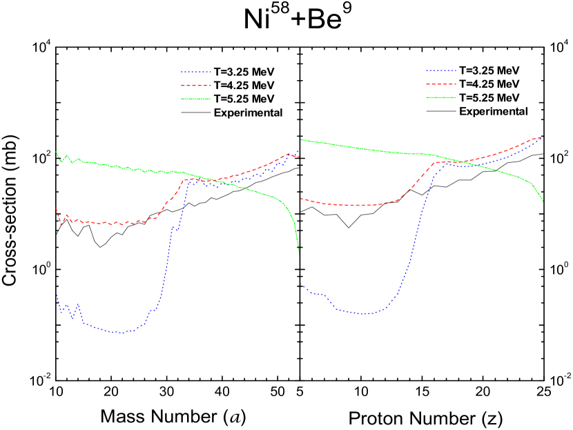
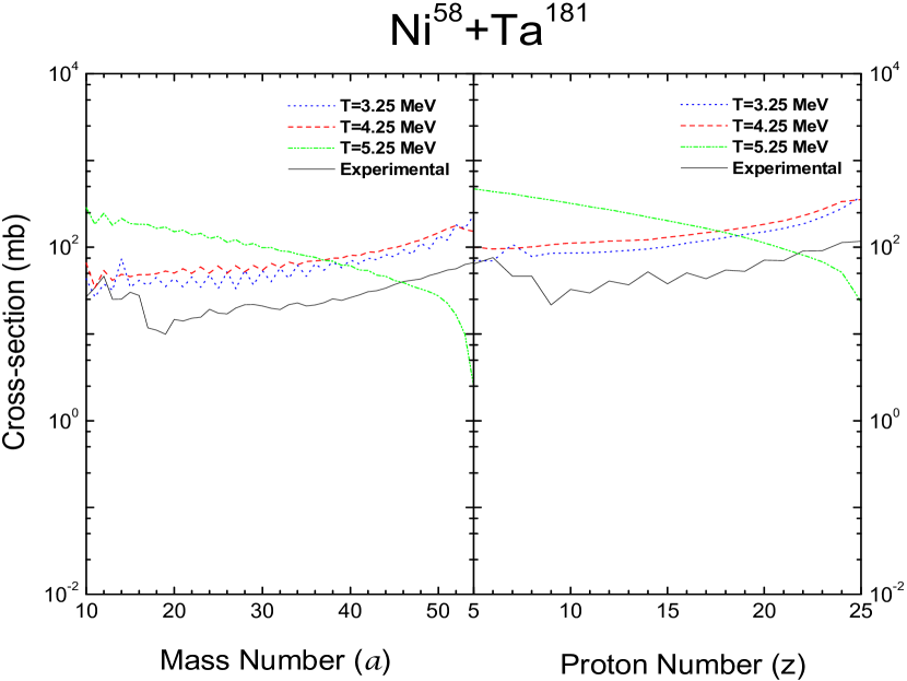
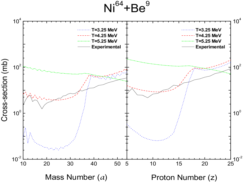
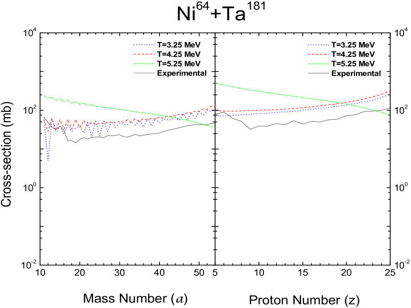
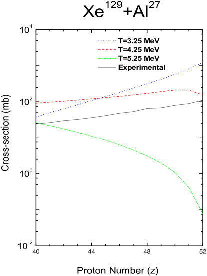
For the case of Xe on Al at 790 MeV/nucleon obvious arguments can be given for defining participants and spectators using straightline geometry. At 140 MeV/nucleon (Ni on Be and Ta) we are probably near the lower limit where this is still an acceptable approximation. An interesting question is: do we expect the same temperature. We fix the temperature from a fit to the experimental cross-sections. As there are many many cross-sections, for fixing the temperature we examine calculated and experimental values of summed cross-sections: $\sigma_{z}\equiv\sum_{n}\sigma(n,z)$ and $\sigma_{a}\equiv\sum_{n+z=a}\sigma(n,z)$. We find that both for Ni on Be and Ta at 140 MeV/nucleon and for Xe on Al at 790 MeV/nucleon we are led to a value of $T\approx 4.25$ MeV. Results are given in the following sections.

At Bevalac where experiments were at higher energies, straight line geometry was used to define participants and spectators down to 250 MeV/ nucleon, the lowest energy for which data are available Gosset .

V Temperature Extraction

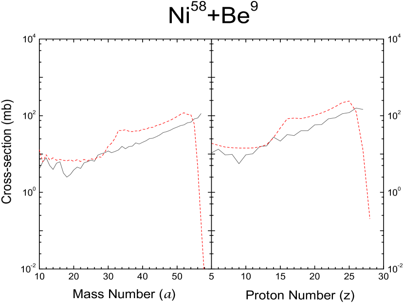
We compute total charge cross-sections $\sigma_{z}=\sum_{n}\sigma(n,z)$ and total mass cross-sections $\sigma_{a}=\sum_{n+z=a}\sigma(n,z)$ and compare with data for ⁵⁸Ni on ⁹Be(fig.1) and ¹⁸¹Ta(fig.2), ⁶⁴Ni on ⁹Be(fig.3) and ¹⁸¹Ta(fig.4) and ¹²⁷Xe on ²⁷Al(fig.5). We show results for $T$=3.25 MeV, 4.25 MeV and 5.25 MeV. The intermediate value of 4.25 MeV fits the multitude of data better than the other two. For brevity we do not show results with other values of temperature in this range. Recall that beam energy has changed from 140 MeV/nucleon to 790 MeV/nucleon and a variety of target-projectile combination has been used but the temperature in the PLF has not moved much which is in accordance with the model of limiting fragmentation.

The results in figs.1-5 do not include very peripheral collisions. For very peripheral collisions lower temperatures should be more appropriate. The use of one temperature for all impact parameters renders our calculation for very peripheral collisions quite inaccurate. We show this in fig.6 where for ⁵⁸Ni+⁹Be we use the same temperature 4.25 MeV for all impact parameters. Beyond $z$=25 our calculation underestimates cross-sections. With $T$=4.25 MeV nuclei produced very close to⁵⁸Ni by abrasion are losing too many nucleons by secondary decay. At a lower $T$ this would get cut down. In this work, from now on, all the results we show pertain to nuclei with at least two nucleons removed from the projectile. In later work we hope to improve upon this. This most likely will require not only a profile in temperature but also a more sophisticated model for abrasion.

VI More Results

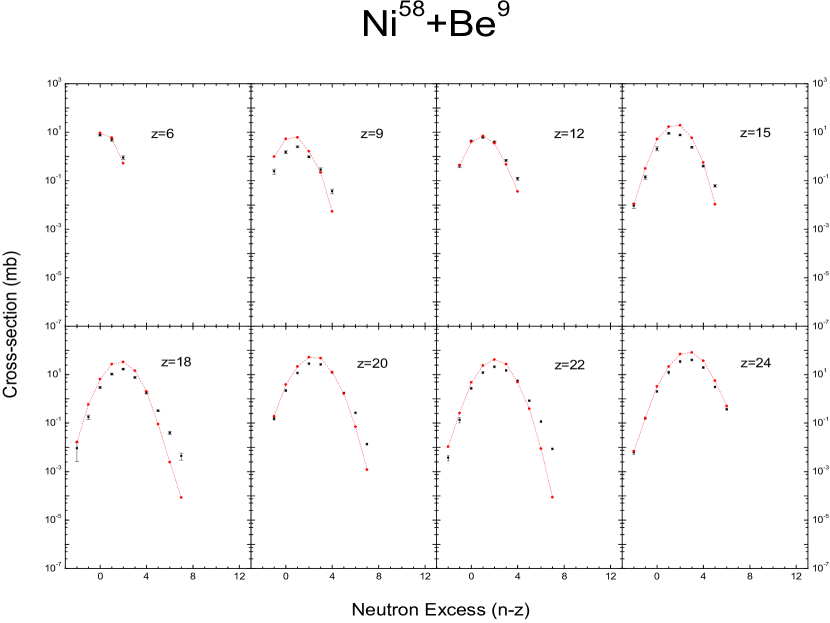
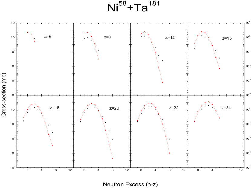
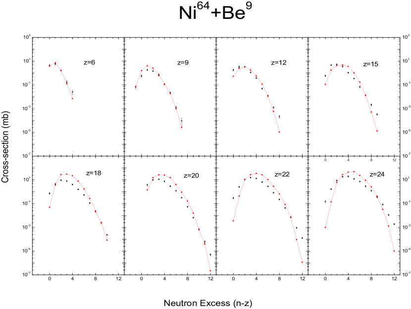
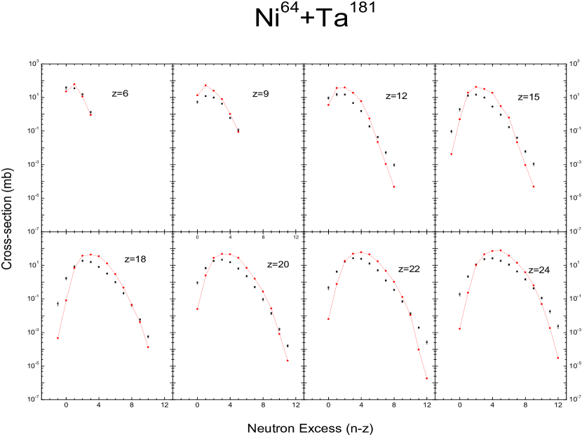
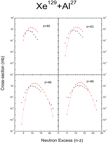
We continue to show results of calculation and compare with experimental data. All calculations are done with $T$=4.25 MeV and freeze-out volume $V=3V_{0}$. The examples shown were picked at random. We pick an isotope characterised by a value of $z$ and plot cross-sections for this $z$ for different values of $n-z$. Fig.7 shows results for the case of ⁵⁸Ni on ⁹Be, fig.8 for ⁵⁸Ni on ¹⁸¹Ta, fig.9 for ⁶⁴Ni on ⁹Be, fig.10 for ⁶⁴Ni on ¹⁸¹Ta and fig.11 for ¹²⁹Xe on ²⁷Al. There are no adjustable parameters any more and the calculated values of the cross-sections are pleasingly close to experimental values. For a given $z$ the general shapes of cross-sections as a function of ($n-z$) are reproduced but in some cases better mapping would be desirable.

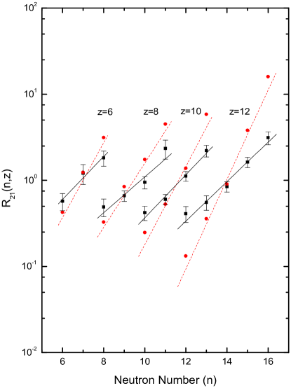
The topic of isoscaling has been much discussed in recent times. We examine if isoscaling follows from our calculation. We know of no obvious reasons why this feature should emerge from this model but it does(fig.12). Let $\sigma_{2}(n,z)$ be the cross-section for producing the nucleus $n,z$ in the reaction ⁶⁴Ni+⁹Be and $\sigma_{1}(n,z)$ be the cross-section for producing the same nucleus in the reaction ⁵⁸Ni+⁹Be. Let $R_{21}(n,z)=\sigma_{2}(n,z)/\sigma_{1}(n,z)$. Experimentally log of $R_{21}(n,z)$ falls on a straightline as a function of $n$ for fixed $z$ and on a different straightline as a function of $z$ for fixed $n$. This is called isoscaling. Fig.12 shows that isoscaling emerges from this model but the slopes of log of $R_{21}$ are overestimated.

If one is looking at isoscaling only and has many more adjustable parameters, better fits to isoscaling data are possible Chaudhuri2 . Our objective here is to look at many other data also simultaneously and we do not have any flexibility. In a recent paper, for the case of ⁵⁸Ni and ⁶⁴Ni on ⁹Be isoscaling parameters were calculated using the HIPSE model Yao .

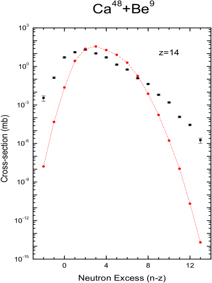
As our last example we consider the production of Si isotopes from the reaction ⁴⁸Ca on ⁹Be at beam energy 140 MeV/nucleon. This was looked at before Chaudhuri6 ; Tsang . There the relative values of cross-sections were calculated using a canonical or a grand canonical model where the temperature was adjusted to get the best fit. For absolute values another constant was needed which was adjusted. Here we show (fig.13) absolute values of cross-sections of Si isotopes with $T$=4.25 MeV and $V=3V_{0}$ as in all our reported calculation above. In expt. the maximum yield is at $n$=16, we get it at $n$=17. The absolute values of the cross-sections at higher yield points agree very well but the shape of the theoretical curve is steeper where the cross-sections are very small.

Several modifications to the model of PLF fragmentation developed here can be considered. One would be a more rigorous choice of $P_{N,Z}(b)$ (eq.(1)). Another would be variation of the temperature $T$ in very peripheral collisions.

VII Summary and Discussion

Calculations reported here suggest that for beam energy upwards of 140 MeV/nucleon an implementable model for projectile fragmentation gives reasonable results for cross-sections of end products. One needs to do an impact parameter integration; at each impact parameter an abraded nucleus is formed at a temperature of about 4.25 MeV. This expands to about three times its original volume and then breaks up thermodynamically into smaller but still hot nuclei. These can further boil off very light particles reaching the end stage. It is rather quick to calculate the abrasion and the thermodynamic break up. Calculating the evaporation of light particles at the last stage takes more time. However we have found that since in the last stage usually there is both a loss and a gain in the population of many composites even without the last stage one has an acceptable measure of cross-sections.

While we have reasonable agreements with many data considered here it is desirable to push the model for improvements. Two obvious goals will be: to find a more sophisticated model of abrasion specially at the low energy end and to build, on physics ground, dependence of temperature on impact parameter for very peripheral collisions. We plan to work on these.

VIII Acknowledgements

This work was supported in part by Natural Sciences and Engineering Research Council of Canada.

Figure 1: Total mass(left panel) and total charge(right panel) cross-section distribution for the ⁵⁸Ni on ⁹Be reaction. The left panel shows the cross-sections as a function of the mass number, while the right panel displays the cross-sections as a function of the proton number. The theoretical results at T=3.25 MeV (dotted line), 4.25 MeV (dashed line) and 5.25 MeV (dash dotted line) are compared with the experimental data (solid line).

Figure 2: Same as Fig. 1 except that here the target is ¹⁸¹Ta instead of ⁹Be.

Figure 3: Same as Fig. 1 except that here the projectile is ⁶⁴Ni instead of ⁵⁸Ni.

Figure 4: Same as Fig. 3 except that here the target is ¹⁸¹Ta instead of ⁹Be.

Figure 5: Total charge cross-section distribution for the ¹²⁹Xe on ²⁷Al reaction. The theoretical results at T=3.25 MeV (dotted line), 4.25 MeV (dashed line) and 5.25 MeV (dash dotted line) are compared with the experimental data (solid line).

Figure 6: Total mass(left panel) and total charge(right panel) cross-section distribution for the ⁵⁸Ni on ⁹Be reaction including the regions coming from the very peripheral collisions. The left panel shows the cross-sections as function of mass number up-to A=58 (i.e. projectile mass) , while the right panel displays cross-sections as function of proton number up-to Z=28 (i.e. proton number of projectile) . The theoretical result at T=4.25 MeV (dashed line) is compared with the experimental data (solid line). As, stated in the text, very peripheral collision should have much lower temperature. The discrepancy between theory and experiment near the end is due to the fact that the same T=4.25 MeV is used even for very peripheral collisions. The evaporative loss from the primary is far too great.

Figure 7: Theoretical isotopic cross-section distribution (circles joined by dashed lines) for ⁵⁸Ni on ⁹Be reaction compared with experimental data (squares with error bars).The temperature used for this calculation is 4.25 MeV.

Figure 8: Same as Fig. 7 except that here the target is ¹⁸¹Ta instead of ⁹Be. The theoretical calculation is done at a temperature T=4.25 MeV.

Figure 9: Same as Fig. 7 except that here the projectile is ⁶⁴Ni instead of ⁵⁸Ni. The temperature used for this calculation is 4.25 MeV.

Figure 10: Same as Fig. 9 except that here the target is ¹⁸¹Ta instead of ⁹Be. The theoretical calculation is done at a temperature T=4.25 MeV.

Figure 11: Same as Fig. 7 except that here the reaction is ¹²⁹Xe on ²⁷Al instead of ⁵⁸Ni on ⁹Be. The temperature used for this calculation is 4.25 MeV.

Figure 12: Theoretical ratios of cross-section (circles) of producing the nucleus(n,z) where reaction 1 is ⁵⁸Ni on ⁹Be and reaction 2 is ⁶⁴Ni on ⁹Be compared with the ratios of the experimental cross-sections of the same two reactions. The dashed and solid lines are the best linear fits of the theoretical and experimental ratios respectively.

Figure 13: Theoretical cross-section distribution (circles joined by dashed line) of silicon isotopes for ⁴⁸Ca on ⁹Be reaction compared with experimental data (squares with error bars). The theoretical calculation is done at a temperature T=4.25 MeV.

References

- (1) M. Mocko,Ph.D. thesis, Michigan State University, 2006.
- (2) M. Mocko et al., Phys. Rev. C78,024612(2008).
- (3) K. Summerer and B. Blank Phys. Rev C61,034607(2000).
- (4) C. B. Das, S. Das Gupta, W. G. Lynch, A. Z. Mekjian and M. B. Tsang, Phys. Rep. 406,1(2005).
- (5) J. P. Bondorf, A. S. Botvina, A. S. Iljinov, I. N. Mishustin, K. Sneppen Phys. Rep 257,133(1995).
- (6) A. S. Botvina, G. Chaudhuri, S Das Gupta and I. N. Mishustin, Phys. Lett B.668,414(2008).
- (7) S. Das Gupta and A. Z. Mekjian,Phys. Rep. 72,131(1981).
- (8) J.-J. Gaimard and K.-H. Schmidt, Nucl. Phys. A531,709,(1991).
- (9) 10.1016/j.nuclphysa.2010.11.001
- (10) V. Weisskopf, Phys. Rev. 52, 295(1937).
- (11) G. Chaudhuri, PhD thesis(Chapter IV), arXiv:nucl-th/0411005
- (12) G. Chaudhuri and S. Das Gupta Phys. Rev. C75,034603(2007).
- (13) G. Chaudhuri, S. Das Gupta and F. Gulminelli, Nucl. Phys. A815,89(2009).
- (14) J. Gosset, H.H.Gutbrod, W.G.Meyer, A.M.Poskanzer, A.Sandoval, R.Stock and G.D.Westfall, Phys. Rev. C16,629(1977).
- (15) Fu Yao et al., Chinese Phys. C33(Suppl.I),126(2009).
- (16) G. Chaudhuri, S. Das Gupta, W. G. Lynch, M. Mocko and M. B. Tsang Phys. Rev C76, 067601(2007).
- (17) M. B. Tsang et al., Phys. Rev. C76,041302(2007).