Spin observables in pion photoproduction
from a unitary and causal effective field theory

Abstract

Pion photoproduction is analyzed with the chiral Lagrangian. Partial-wave amplitudes are obtained by an analytic extrapolation of subthreshold reaction amplitudes computed in chiral perturbation theory, where the constraints set by electromagnetic-gauge invariance, causality and unitarity are used to stabilize the extrapolation. The experimental data set is reproduced up to energies $\sqrt{s}\simeq 1300$ MeV in terms of the parameters relevant at order $Q^{3}$. We present and discuss predictions for various spin observables.

1 Introduction

Chiral perturbation theory is a systematic tool for studying low-energy hadron dynamics. Particularly pion-nucleon scattering and pion photoproduction were considered in [1, 2, 3, 4]. The application of $\chi$PT is however limited to the near threshold region. A method to extrapolate $\chi$PT results beyond the threshold region using analyticity and unitarity constraints was proposed recently in [5]. We focus on results obtained for pion photoproduction. The predictions for spin observables as currently being measured at MAMI are confronted with previous theoretical predictions.

2 Chiral symmetry, causality and unitarity

Our approach is based on the chiral Lagrangian involving pion, nucleon and photon fields [4, 2]. The terms relevant at the order $Q^{3}$ for pion elastic scattering and pion photoproduction are listed below

$$\mathcal{L}_{int} = -\frac{1}{4\,f^{2}}\,\bar{N}\,\gamma^{\mu}\,\big{(}\vec{\tau}\cdot\big{(}\vec{\pi}\times(\partial_{\mu}\vec{\pi})\big{)}\big{)}\,N+\frac{g_{A}}{2\,f}\,\bar{N}\,\gamma_{5}\,\gamma^{\mu}\,\big{(}\vec{\tau}\cdot(\partial_{\mu}\vec{\pi})\big{)}\,N$$ (1)

$$- e\,\Big{\{}\big{(}\vec{\pi}\times(\partial_{\mu}\vec{\pi})\big{)}_{3}+\bar{N}\,\gamma_{\mu}\,\frac{1+\tau_{3}}{2}\,N-\frac{g_{A}}{2\,f}\,\bar{N}\,\gamma_{5}\,\gamma_{\mu}\,\big{(}\vec{\tau}\times\vec{\pi}\big{)}_{3}\,N\Big{\}}\,A^{\mu}$$

$$- \frac{e}{4\,m_{N}}\,\bar{N}\,\sigma_{\mu\nu}\,\frac{\kappa_{s}+\kappa_{v}\,\tau_{3}}{2}\,N\,F^{\mu\nu}+\frac{e^{2}}{32\pi^{2}f}\,\epsilon^{\mu\nu\alpha\beta}\,\pi_{3}\,F_{\mu\nu}\,F_{\alpha\beta}$$

$$- \frac{2\,c_{1}}{f^{2}}\,m_{\pi}^{2}\,\bar{N}\,(\vec{\pi}\cdot\vec{\pi})\,N-\frac{c_{2}}{2\,f^{2}\,m_{N}^{2}}\,\Big{\{}\bar{N}\,(\partial_{\mu}\,\vec{\pi})\cdot(\partial_{\nu}\vec{\pi})\,(\partial^{\mu}\partial^{\nu}N)+\rm{h.c.}\Big{\}}$$

$$+ \frac{c_{3}}{f^{2}}\,\bar{N}\,(\partial_{\mu}\,\vec{\pi})\cdot(\partial^{\mu}\vec{\pi})\,N-\frac{c_{4}}{2\,f^{2}}\,\bar{N}\,\sigma^{\mu\nu}\,\big{(}\vec{\tau}\cdot\big{(}(\partial_{\mu}\vec{\pi})\times(\partial_{\nu}\vec{\pi})\big{)}\big{)}\,N$$

$$- i\,\frac{d_{1}+d_{2}}{f^{2}\,m_{N}}\,\bar{N}\,\big{(}\vec{\tau}\cdot\big{(}(\partial_{\mu}\vec{\pi})\times(\partial_{\nu}\partial_{\mu}\vec{\pi})\big{)}\big{)}\,(\partial^{\nu}N)+\rm{h.c.}$$

$$+ \frac{i\,d_{3}}{f^{2}\,m_{N}^{3}}\,\bar{N}\,\big{(}\vec{\tau}\cdot\big{(}(\partial_{\mu}\vec{\pi})\times(\partial_{\nu}\partial_{\lambda}\vec{\pi})\big{)}\big{)}\,(\partial^{\nu}\partial^{\mu}\partial^{\lambda}N)+\mbox{h.c.}$$

$$- 2\,i\,\frac{m_{\pi}^{2}\,d_{5}}{f^{2}\,m_{N}}\,\bar{N}\,\big{(}\vec{\tau}\cdot\big{(}\vec{\pi}\times(\partial_{\mu}\vec{\pi})\big{)}\big{)}\,(\partial^{\mu}N)+\rm{h.c.}$$

$$- \frac{i\,e}{f\,m_{N}}\,\epsilon^{\mu\nu\alpha\beta}\,\bar{N}\,\big{(}d_{8}\,(\partial_{\alpha}\,\pi_{3})+d_{9}\,\big{(}\vec{\tau}\cdot(\partial_{\alpha}\vec{\pi})\big{)}\big{)}\,(\partial_{\beta}\,N)\,F_{\mu\nu}+\mbox{h.c.}$$

$$+ i\,\frac{d_{14}-d_{15}}{2\,f^{2}\,m_{N}}\,\bar{N}\,\sigma^{\mu\nu}\,\big{(}(\partial_{\nu}\vec{\pi})\cdot(\partial_{\mu}\partial_{\lambda}\vec{\pi})\big{)}\,(\partial^{\lambda}N)+\mbox{h.c.}$$

$$- \frac{m_{\pi}^{2}\,d_{18}}{f}\,\bar{N}\,\gamma_{5}\,\gamma^{\mu}\,\big{(}\vec{\tau}\cdot(\partial_{\mu}\vec{\pi})\big{)}\,N-\frac{e\,m_{\pi}^{2}\,d_{18}}{f}\,\bar{N}\,\gamma_{5}\,\gamma^{\mu}\,\big{(}\vec{\tau}\times\vec{\pi}\big{)}_{3}\,N\,A_{\mu}$$

$$+ \frac{e\,(d_{22}-2\,d_{21})}{2\,f}\,\bar{N}\,\gamma_{5}\,\gamma^{\mu}\,\big{(}\vec{\tau}\times\partial^{\nu}\,\vec{\pi}\big{)}_{3}\,N\,F_{\mu\nu}$$

$$+ \frac{e\,d_{20}}{2\,f\,m_{N}^{2}}\,\bar{N}\,\gamma_{5}\,\gamma^{\mu}\,\big{(}\vec{\tau}\times(\partial_{\lambda}\,\vec{\pi})\big{)}_{3}\,(\partial^{\nu}\partial^{\lambda}N)\,F_{\mu\nu}+\mbox{h.c.}\,.$$

A strict chiral expansion of the amplitude to the order $Q^{3}$ includes tree-level graphs, loop diagrams, and counter terms. Counter terms depend on a few unknown parameters, which we adjusted to the empirical data on $\pi N$ elastic scattering and pion photoproduction. The extrapolation of the amplitudes obtained within ChPT is performed utilizing constraints imposed by basic principles of analyticity and unitarity. For each partial wave we solved the non-linear integral equation

$$T_{ab}^{JP}(\sqrt{s}\,)=U_{ab}^{JP}(\sqrt{s}\,)$$

$$\qquad+\sum_{c,d}\int_{\mu_{\rm thr}}^{\infty}\frac{dw}{\pi}\frac{\sqrt{s}-\mu_{M}}{w-\mu_{M}}\frac{T_{ac}^{*,JP}(w)\,\rho^{JP}_{cd}(w)\,T_{db}^{JP}(w)}{w-\sqrt{s}-i\epsilon}\,,$$ (2)

where the generalized potential, $U_{ab}^{(JP)}(\sqrt{s}\,)$, is the part of the amplitude that contains left-hand cuts only. The phase-space matrix $\rho^{JP}_{cd}(w)$ reflects our particular convention for the partial-wave amplitudes, that are free of kinematical constraints. The matching scale $\mu_{M}$ is required as to arrive at approximate crossing symmetric results. For more details we refer to [5].

3 Results

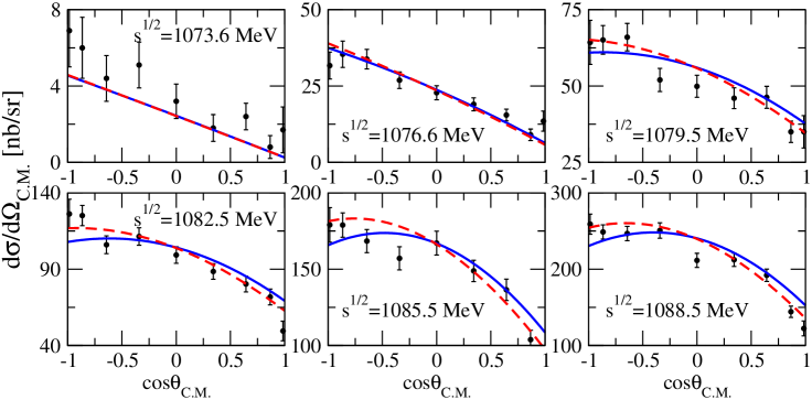
Figure 1: Near threshold differential cross section for the reaction $\gamma p\to\pi^{0}p$ with data taken from [6, 7]. Shown are results from our coupled-channel theory including isospin breaking effects as are implied by the use of empirical pion and nucleon masses. The solid lines correspond to our calculation with only $s$- and $p$-wave multipoles included. The effect of higher partial waves is shown by the dashed lines.

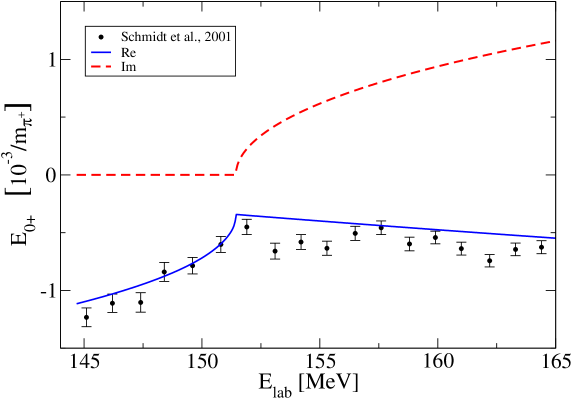
Figure 2: Energy dependence of the $E_{0+}$ multipole close to the pion production threshold. The data are from [7].

The low-energy constants relevant for the elastic pion-nucleon scattering were determined in [5]. The empirical $s$- and $p$-wave phase shifts are well reproduced up to the energy $\sqrt{s}\approx 1300$ MeV. Above this energy inelastic channels become important. The only exception is the $P_{11}$ partial wave where the influence of inelastic channels is significantly larger, that results in a slightly worse description of the phase shift. A convincing convergence pattern when going from $Q^{1}$ to $Q^{3}$ calculation was observed. In addition to the low-energy constants of the Lagrangian (1) there are CDD pole parameters characterizing the Delta and Roper resonances [5].

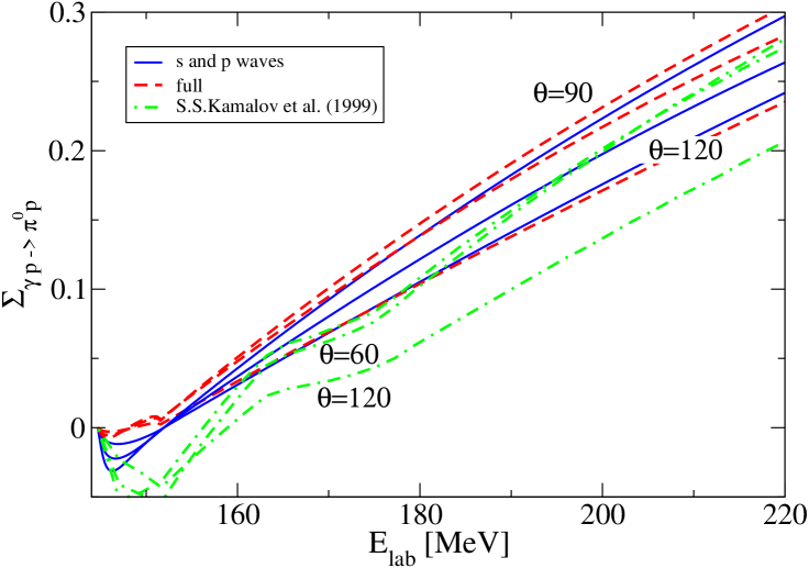
Figure 3: Energy dependence of the beam asymmetry for three particular angles.

The pion-photoproduction $s$- and $p$-wave multipoles are quite constrained. There are only four additional low-energy constants and four CDD-pole parameters for the twelve multipoles to be reproduced. Nevertheless a good agreement to the existing partial wave analyzes was achieved. In order to avoid the ambiguities in the different partial-wave analyzes we determined the parameters from the experimental data directly, where we excluded the near-threshold data in the fit. Our results for the differential cross sections, beam asymmetries, and helicity asymmetry for the reaction channels $\gamma p\to\pi^{0}p$, $\gamma p\to\pi^{+}n$, $\gamma n\to\pi^{-}p$ are in agreement with experimental data from threshold up to $\sqrt{s}=1300$ MeV. Fig. 1 confronts our prediction for the neutral pion-photo production with the near-threshold MAMI data [6, 7]. This data allows one to extract the electric $s$-wave multipole $E_{0+}$. Its energy dependence reveals a prominent cusp effect at the opening of the $\pi^{+}n$ channel. As shown Fig. 2 this structure is reproduced by our calculation, which discriminates the channels with neutral and charged pions.

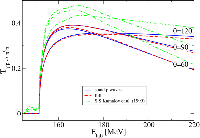
Figure 4: Energy dependence of the target asymmetry for three particular angles.

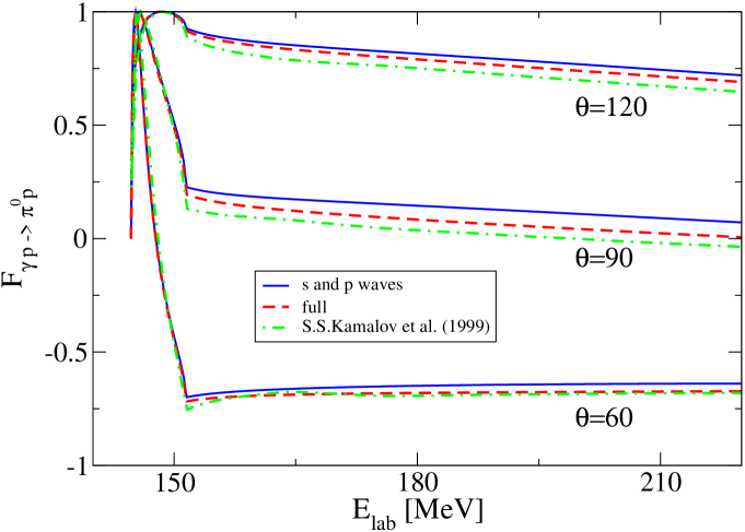
Figure 5: Energy dependence of the double polarization observable $F$ for three particular angles.

Further information about the low-energy photoproduction dynamics is encoded in the $p$-wave threshold multipoles. In order to disentangle the three independent $p$-wave amplitudes it is insufficient to measure the differential cross section only. The near-threshold beam asymmetry in $\gamma p\to\pi^{0}p$ was measured by MAMI [7]. Our results are in striking disagreement with that measurement. We predict the beam asymmetry to change sign close to threshold, in a similar manner as predicted before in the dynamical model of Kamalov et al. [8]. In Fig. 3 we compare the two different results on the beam asymmetry. Though there is qualitative agreement, important quantitative differences remain. It is interesting to observe that d-wave multipoles appear to play an important role in the near-threshold region. This was discussed also in [9]. Thus the beam asymmetry may not be the optimal quantity to extract the p-wave threshold amplitudes. Currently a new data set on the beam asymmetry is being analyzed at MAMI.

We conclude that it is important to take further data on spin observables other than the beam asymmetry. Two cases are currently been studied at MAMI close to threshold. The target asymmetry $T$ and the double polarization observable $F$. Since there are different phase conventions used in the literature the reader may appreciate that we detail the relevant expression in the convention used in [5]. It holds

$$\frac{d\sigma}{d\Omega}=\frac{\bar{p}_{\rm cm}}{2\,p_{\rm cm}}\left(|H_{N}|^{2}+|H_{SA}|^{2}+|H_{SP}|^{2}+|H_{D}|^{2}\right)\,,$$

$$\Sigma\,\frac{d\sigma}{d\Omega}=\frac{\bar{p}_{\rm cm}}{p_{\rm cm}}\,\Re\left(H_{SP}H_{SA}^{*}-H_{N}H_{D}^{*}\right)\,,$$

$$T\,\frac{d\sigma}{d\Omega}=\frac{\bar{p}_{\rm cm}}{p_{\rm cm}}\,\Im\left(H_{SP}H_{N}^{*}+H_{D}H_{SA}^{*}\right)\,,$$

$$F\,\frac{d\sigma}{d\Omega}=\frac{\bar{p}_{\rm cm}}{p_{\rm cm}}\,\Re\left(H_{SP}H_{N}^{*}+H_{D}H_{SA}^{*}\right)\,,$$ (3)

with $x=\cos\theta$ and

$$H_{N\;\;}=\frac{m_{N}}{4\pi\,\sqrt{s}}\,\cos\frac{\theta}{2}\,\sum_{J}\left(t^{J}_{+,1}-t^{J}_{-,1}\right)\left(P^{\prime}_{J+\frac{1}{2}}(x)-P^{\prime}_{J-\frac{1}{2}}(x)\right)\,,$$

$$H_{SA}=-\frac{m_{N}}{4\pi\,\sqrt{s}}\,\sin\frac{\theta}{2}\,\sum_{J}\left(t^{J}_{+,1}+t^{J}_{-,1}\right)\left(P^{\prime}_{J+\frac{1}{2}}(x)+P^{\prime}_{J-\frac{1}{2}}(x)\right)\,,$$

$$H_{SP}=\frac{m_{N}}{4\pi\,\sqrt{s}}\,\frac{-\sin\theta\cos{\frac{\theta}{2}}}{\sqrt{(J-\frac{1}{2})(J+\frac{3}{2})}}\,\sum_{J}\left(t^{J}_{+,2}-t^{J}_{-,2}\right)\left(P^{\prime\prime}_{J+\frac{1}{2}}(x)-P^{\prime\prime}_{J-\frac{1}{2}}(x)\right)\,,$$

$$H_{D\;\;}=\frac{m_{N}}{4\pi\,\sqrt{s}}\,\frac{\sin\theta\sin{\frac{\theta}{2}}}{\sqrt{(J-\frac{1}{2})(J+\frac{3}{2})}}\,\sum_{J}\left(t^{J}_{+,2}+t^{J}_{-,2}\right)\left(P^{\prime\prime}_{J+\frac{1}{2}}(x)+P^{\prime\prime}_{J-\frac{1}{2}}(x)\right)\,.$$

In Fig. 4 an Fig. 5 we show our predictions for the energy dependence of the target asymmetry and the $F$ observable in comparison with the predictions of the dynamical model of Ref. [8] calculated at different angles. One can see that the target and beam asymmetry are most sensitive to the details of the dynamics, whereas the $F$ observable is quite similar in both approaches.

In order to unravel the dynamics close to threshold we detail the contributions of $s$- and $p$-waves to the differential cross section and the $\Sigma$, $T$ and $F$ observables. It holds

$$\frac{d\sigma}{d\Omega} = \frac{\bar{p}_{\rm cm}}{p_{\rm cm}}\,\Big{[}|E_{0+}|^{2}+\frac{1}{2}\,|P_{2}|^{2}+\frac{1}{2}\,|P_{3}|^{2}+2\,\Re(E_{0+}\,P_{1}^{*})\,\cos{\theta}$$

$$+ \Big{(}|P_{1}|^{2}-\frac{1}{2}\,|P_{2}|^{2}-\frac{1}{2}\,|P_{3}|^{2}\Big{)}\,\cos^{2}{\theta}\Big{]}\,,$$

$$\Sigma\,\frac{d\sigma}{d\Omega} = \frac{\bar{p}_{\rm cm}}{2\,p_{\rm cm}}\,\big{[}|P_{3}|^{2}-|P_{2}|^{2}\big{]}\,\sin^{2}{\theta}\,,$$

$$T\,\frac{d\sigma}{d\Omega} = -\frac{\bar{p}_{\rm cm}}{p_{\rm cm}}\,\Im{\big{[}(E_{0+}+P_{1}\cos{\theta})\,(P_{2}-P_{3})^{*}\big{]}}\sin{\theta}\,,$$

$$F\,\frac{d\sigma}{d\Omega} = \frac{\bar{p}_{\rm cm}}{p_{\rm cm}}\,\Re{\big{[}(E_{0+}+P_{1}\cos{\theta})\,(P_{2}-P_{3})^{*}\big{]}}\sin{\theta},$$ (4)

with the linear combinations of $p$-wave multipoles $P_{1}=3\,E_{1+}+M_{1+}-M_{1-}$, $P_{2}=3\,E_{1+}-M_{1+}+M_{1-}$, $P_{3}=2\,M_{1+}+M_{1-}$.

The expression for the target asymmetry $T$ (Eq. (4)) depends on the imaginary parts of the multipoles. That is why close to the $\pi^{0}p$ threshold $T$ is very small (see Fig. 4). Slightly above the $\pi^{+}n$ threshold it holds approximately

$$T\,\frac{d\sigma}{d\Omega}(\theta=90^{\circ})\approx-\frac{\bar{p}_{\rm cm}}{p_{\rm cm}}\,\Im{(E_{0+})}\,(P_{2}-P_{3})\,,$$ (5)

since the imaginary parts of $p$-wave multipoles are small. The imaginary part of $E_{0+}$ is in turn dominated by the intermediate $\pi^{+}n$ state. This allows one to access the difference $P_{2}-P_{3}$ in the vicinity of the $\pi^{+}n$ threshold.

In the beam asymmetry $\Sigma$ the $p$-waves multipoles enter only quadratically and therefore terms containing an interference of the $E_{0+}$ and $d$-wave amplitudes are not suppressed by powers of the $\pi N$ momentum. Moreover the magnitudes of $|P_{2}|$ and $|P_{3}|$ are similar [7] which further diminishes the relative importance of the $p$-wave contribution to $\Sigma$. In contrast, the quantity $F(\theta=90^{\circ})$ contains the term $\Re{\left(E_{0+}\,(P_{2}-P_{3})^{*}\right)}$ but no other competing contribution. Thus measuring $F$ provides a reliable determination of $P_{2}-P_{3}$. Note that this difference is not small because $P_{2}$ and $P_{3}$ have opposite signs [7].

4 Summary

We studied pion photoproduction from threshold up to $\sqrt{s}=1300$ MeV with a novel approach developed in [5] based on an analytic extrapolation of subthreshold amplitudes calculated in ChPT. The free parameters were adjusted to the pion-nucleon and photoproduction empirical data excluding the threshold region. Nevertheless the near-threshold MAMI data on the reaction $\gamma p\to\pi^{0}p$ are described well. The energy dependence of the $s$-wave electric $E_{0+}$ multipole close to threshold including its prominent cusp structure is also well reproduced. We presented predictions for spin observables that are planned to be measured or being analyzed at MAMI. Our predictions are compared with results of the dynamical model of Kamalov et al. [8]. The importance of $d$-waves for the beam asymmetry close to the $\pi N$ threshold was emphasized. This effect indicates that the beam asymmetry may be not best suited to disentangle the various $p$-wave threshold multipoles as has been anticipated before. We argued that the measurement of the double polarization observable $F$ suits this purpose much better.

Acknowledgments

We thank M. Ostrick and L. Tiator for stimulating discussions.

References

• [1] V.Β Bernard, N.Β Kaiser, U.-G. Meissner, Chiral dynamics in nucleons and nuclei, Int. J. Mod. Phys. E4 (1995) 193–346.
• [2] V.Β Bernard, Chiral Perturbation Theory and Baryon Properties, Prog. Part. Nucl. Phys. 60 (2008) 82–160.
• [3] V.Β Bernard, N.Β Kaiser, U.-G. Meissner, Determination of the low-energy constants of the next-to- leading order chiral pion nucleon Lagrangian, Nucl. Phys. A615 (1997) 483–500.
• [4] N.Β Fettes, U.-G. Meissner, S.Β Steininger, Pion nucleon scattering in chiral perturbation theory. I: Isospin-symmetric case, Nucl. Phys. A640 (1998) 199–234.
• [5] A.Β Gasparyan, M.Β Lutz, Photon- and pion-nucleon interactions in a unitary and causal effective field theory based on the chiral Lagrangian, Nucl.Phys. A848 (2010) 126–182.
• [6] A.Β Schmidt, PhD thesis, Mainz (2001), http://wwwa2.kph.uni-maiz.de/A2/.
• [7] A.Β Schmidt, etΒ al., Test of low-energy theorems for p(gamma(pol.),pi0)p in the threshold region, Phys. Rev. Lett. 87 (2001) 232501.
• [8] S.Β S. Kamalov, G.-Y. Chen, S.-N. Yang, D.Β Drechsel, L.Β Tiator, pi0 photo- and electroproduction at threshold within a dynamical model, Phys. Lett. B522 (2001) 27–36.
• [9] C.Β Fernandez-Ramirez, A.Β M. Bernstein, T.Β W. Donnelly, The unexpected impact of D waves in low-energy neutral pion photoproduction from the proton and the extraction of multipoles, Phys. Rev. C80 (2009) 065201.