Affine-invariant diffusion geometry for the analysis of deformable 3D shapes

Abstract

We introduce an (equi-)affine invariant diffusion geometry by which surfaces that go through squeeze and shear transformations can still be properly analyzed. The definition of an affine invariant metric enables us to construct an invariant Laplacian from which local and global geometric structures are extracted. Applications of the proposed framework demonstrate its power in generalizing and enriching the existing set of tools for shape analysis.

1 Introduction

Diffusion geometry is an umbrella term referring to geometric analysis of diffusion or random walk processes. Such methods, first introduced in theoretical geometry [3] have matured into practical applications in the fields of manifold learning [7] and shape analysis [11]. In the shape analysis community, diffusion geometry methods were used to define low-dimensional representations for manifolds [7, 21], build intrinsic distance metrics and construct shape distribution descriptors [21, 12], define spectral signatures [20] (shape-DNA), and local descriptors [23]. Diffusion embeddings were used for finding correspondence between shapes [13] and detecting intrinsic symmetries [18] . In many settings, the construction of diffusion geometry boils down to the definition of a Laplacian operator. Such an operator should possess certain invariance properties desired in a specific application.

In this paper, we construct (equi-)affine-invariant diffusion geometry for 3D shapes. Affine invariance is important in many applications in the analysis of images [15] and 3D shapes [9]. We first construct an affine-invariant Riemannian metric that allows us define an affine-invariant Laplacian, with which we in turn define affine invariant diffusion geometry for surfaces. This new geometry enables efficient computational tools that handle both non-rigid approximately-isometric deformations of the surface together with equi-affine transformations of the embedding space. We demonstrate the usefulness of our construction in a range of shape analysis applications, such as retrieval, correspondence, and symmetry detection.

2 Background

Let $X$ denote a compact two-dimensional Riemannian manifold (possibly with boundary) representing the outer boundary of a physical solid object in the 3D space. The Riemannian metric tensor $g$ is defined as a local inner product $\langle\cdot,\cdot\rangle_{x}$ on the tangent plane $T_{x}X$ at each point $x\in X$. Given a smooth scalar field $f:X\rightarrow\mathbb{R}$, its gradient $\nabla f$ at point $x$ is defined through the relation $f(x+dr)=f(x)+\langle\nabla f(x),dr\rangle_{x}$, where $dr\in T^{*}_{x}X$ is an infinitesimal tangent vector. The positive semi-definite self-adjoint Laplace-Beltrami operator $\Delta_{g}$ associated with the metric tensor $g$ is defined by the identity

$$\int f\Delta_{g}h\,da = -\int\langle\nabla f,\nabla h\rangle_{x}da$$ (1)

holding for any pair of smooth scalar fields $f,h:X\rightarrow\mathbb{R}$; here $da$ denotes the standard area measure on $X$. Whenever possible, we will omit the subscript $g$ and refer to the Laplace-Beltrami operator simply as to $\Delta$.

Assuming further that the manifold is embedded isometrically in $\mathbb{R}^{3}$ and (possibly, locally) parametrized by a regular map $\mathbf{x}:U\rightarrow{\mathbb{R}}^{3}$ over a planar domain $U$, the metric tensor $g$ assumes the form of a $2\times 2$ positive-definite matrix called the first fundamental form, whose elements are given by the inner products $g_{ij}=\frac{\partial\mathbf{x}^{\mathrm{T}}}{\partial u_{i}}\frac{\partial\mathbf{x}}{\partial u_{j}}$.

The Laplace-Beltrami operator can be expressed in the parametrization coordinates as

$$\Delta = -\frac{1}{\sqrt{g}}\partial_{i}\sqrt{g}g^{ij}\partial_{j},$$ (2)

where we use Einstein’s summation convention, according to which $g=\mathrm{det}(g_{ij})$ denotes the determinant of the metric, $g^{ij}$ are the components of the inverse metric tensor, and repeated indices are summed over. When the metric is Euclidean ($g_{ij}=\mathbf{I}$), the operator reduces to the familiar $\Delta f=-\left(\frac{\partial^{2}f}{\partial u^{2}_{1}}+\frac{\partial^{2}f}{\partial u^{2}_{2}}\right)$ (note that we define the Laplacian with the minus sign in order to ensure its positive semi-definiteness).

The Laplace-Beltrami operator gives rise to the partial differential equation

$$\left(\frac{\partial}{\partial t}+\Delta\right)f(t,x)=0,$$ (3)

called the heat equation. The heat equation describes the propagation of heat on the surface and its solution $f(t,x)$ is the heat distribution at a point $x$ in time $t$. The initial condition of the equation is some initial heat distribution $f(0,x)$; if $X$ has a boundary, appropriate boundary conditions must be added. The solution of (3) corresponding to a point initial condition $f(0,x)=\delta(x-x^{\prime})$, is called the heat kernel and represents the amount of heat transferred from $x$ to $x^{\prime}$ in time $t$ due to the diffusion process. Using spectral decomposition, the heat kernel can be represented as

$$h_{t}(x,x^{\prime}) = \sum_{i\geq 0}e^{-\lambda_{i}t}\phi_{i}(x)\phi_{i}(x^{\prime})$$ (4)

where $\phi_{i}$ and $\lambda_{i}$ are, respectively, the eigenfunctions and eigenvalues of the Laplace-Beltrami operator satisfying $\Delta\phi_{i}=\lambda_{i}\phi_{i}$ (without loss of generality, we assume $\lambda_{i}$ to be sorted in increasing order starting with $\lambda_{0}=0$). Since the Laplace-Beltrami operator is an intrinsic geometric quantity, i.e., it can be expressed solely in terms of the metric of $X$, its eigenfunctions and eigenvalues as well as the heat kernel are invariant under isometric transformations of the manifold.

The value of the heat kernel $h_{t}(x,x^{\prime})$ can be interpreted as the transition probability density of a random walk of length $t$ from the point $x$ to the point $x^{\prime}$. This allows to construct a family of intrinsic metrics known as diffusion metrics,

$$d^{2}_{t}(x,x^{\prime})=\int\left(h_{t}(x,\cdot)-h_{t}(x^{\prime},\cdot)\right)^{2}da=\sum_{i>0}e^{-\lambda_{i}t}(\phi_{i}(x)-\phi_{i}(x^{\prime}))^{2},$$ (5)

which measure the “connectivity rate” of the two points by paths of length $t$.

The parameter $t$ can be given the meaning of scale, and the family $\{d_{t}\}$ can be thought of as a scale-space of metrics. By integrating over all scales, a scale-invariant version of (5) is obtained,

$$d_{\mathrm{CT}}^{2}(x,x^{\prime}) = 2\int_{0}^{\infty}d_{t}^{2}(x,x^{\prime})dt=\sum_{i>0}\frac{1}{\lambda_{i}}(\phi_{i}(x)-\phi_{i}(x^{\prime}))^{2}.$$ (6)

This metric is referred to as the commute-time distance and can be interpreted as the connectivity rate by paths of any length. We will broadly call constructions related to the heat kernel, diffusion and commute time metrics as diffusion geometry.

3 Affine-invariant diffusion geometry

An affine transformation $\mathbf{x}\mapsto\mathbf{A}\mathbf{x}+\mathbf{b}$ of the three-dimensional Euclidean space can be parametrized by a regular $3\times 3$ matrix $\mathbf{A}$ and a $3\times 1$ vector $\mathbf{b}$ since all constructions discussed here are trivially translation invariant, we will omit the vector $\mathbf{b}$. The transformation is called special affine or equi-affine if it is volume-preserving, i.e., $\det\mathbf{A}=1$.

As the standard Euclidean metric is not affine-invariant, the Laplace-Beltrami operators associated with $X$ and $\mathbf{A}X$ are generally distinct, and so are the resulting diffusion geometries. In what follows, we are going to substitute the Euclidean metric by its equi-affine invariant counterpart. That, in turn, will induce an equi-affine-invariant Laplace-Beltrami operator and define equi-affine-invariant diffusion geometry.

The equi-affine metric can be defined through the parametrization of a curve [1, 4, 5, 6, 16, 22]. Let $C$ be a curve on $X$ parametrized by $p$. By the chain rule,

$$\frac{dC}{dp} = \mathbf{x}_{1}\frac{du_{1}}{dp}+\mathbf{x}_{2}\frac{du_{2}}{dp}$$

$$\frac{d^{2}C}{dp^{2}} = \mathbf{x}_{1}\frac{d^{2}u_{1}}{dp^{2}}+\mathbf{x}_{2}\frac{d^{2}u_{2}}{dp^{2}}+\mathbf{x}_{11}\left(\frac{du_{1}}{dp}\right)^{2}+2\mathbf{x}_{12}\frac{du_{1}}{dp}\frac{du_{2}}{dp}+\mathbf{x}_{22}\left(\frac{du_{2}}{dp}\right)^{2},$$ (7)

where, for brevity, we denote $\mathbf{x}_{i}=\frac{\partial\mathbf{x}}{\partial u_{i}}$ and $\mathbf{x}_{ij}=\frac{\partial^{2}\mathbf{x}}{\partial u_{i}\partial u_{j}}$. As volumes are preserved under the equi-affine group of transformations, we define the invariant arclength $p$ through

$$\det(\mathbf{x}_{1},\mathbf{x}_{2},C_{pp}) = 1.$$ (8)

Plugging (7) into (8) yields

$$dp^{2}=\det(\mathbf{x}_{1},\mathbf{x}_{2},\mathbf{x}_{11}du_{1}^{2}+2\mathbf{x}_{12}du_{1}du_{2}+\mathbf{x}_{22}du_{2}^{2}),$$ (9)

from where we readily have an equi-affine-invariant pre-metric tensor

$$\hat{g}_{ij} = \tilde{g}_{ij}\left|\tilde{g}\right|^{-1/4},$$ (10)

where $\tilde{g}_{ij}=\det(\mathbf{x}_{1},\mathbf{x}_{2},\mathbf{x}_{ij})$. The pre-metric tensor (10) defines a true metric only on strictly convex surfaces [5]; in more general cases, it might cease from being positive definite. In order to deal with arbitrary surfaces, we extend the metric definition by restricting the eigenvalues of the tensor to be positive. Representing $\hat{g}$ as a $2\times 2$ matrix admitting the eigendecomposition $\hat{\mathbf{G}}=\mathbf{U}\mathbf{\Gamma}\mathbf{U}^{\mathrm{T}}$, where $\mathbf{U}$ is orthonormal and $\mathbf{\Gamma}=\mathrm{diag}\{\gamma_{1},\gamma_{2}\}$, we compose a new first fundamental form matrix $\mathbf{G}=\mathbf{U}|\mathbf{\Gamma}|\mathbf{U}^{\mathrm{T}}$. The corresponding metric tensor $g$ is positive definite and is equi-affine invariant.

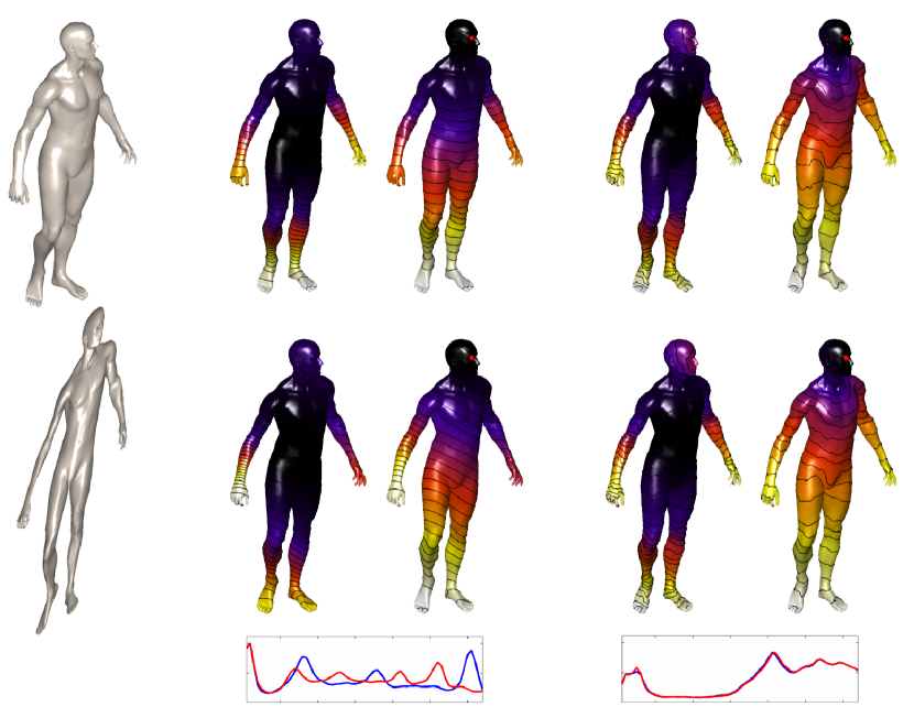
Figure 3: Heat kernel signature $h_{t}(x,x)$ and diffusion metric ball (second and third columns, respectively), and their affine-invariant counterparts (fourth and fifth columns, respectively). Two rows show a shape and its equi-affine transformation. For convenience of visualization, the kernel and the metric are overlaid onto the untransformed shape. Plots under the figure show the corresponding metric distributions before and after the transformation.

Plugging this $g$ into (1), we obtain an equi-affine-invariant Laplace-Beltrami operator $\Delta_{g}$. Such an operator defines an equi-affine-invariant diffusion geometry, i.e., the eigenfunction, heat kernel, and diffusion metrics it generates remain unaltered by a global volume-preserving affine transformation of the shape (Figures 2–3).

4 Discretization

In order to compute the equi-affine metric we need to evaluate the second-order derivatives of the surface with respect to some parametrization coordinates. While this can be done practically in any representation, here we assume that the surface is given as a triangular mesh. For each triangular face, the metric tensor elements are calculated from a quadratic surface patch fitted to the triangle itself and its three adjacent neighbor triangles. The four triangles are unfolded to the plane, to which an affine transformation is applied in such a way that the central triangle becomes a unit simplex. The coordinates of this planar representation are used as the parametrization $\mathbf{u}$ with respect to which the first fundamental form coefficients are computed at the barycenter of the simplex (Figure 1). This step is performed for every triangle of the mesh.

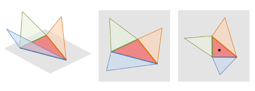
Figure 1: Left to right: part of a triangulated surface about a specific triangle. The three neighboring triangles together with the central one are unfolded flat to the plane. The central triangle is canonized into a right isosceles triangle; three neighboring triangles follow the same planar affine transformation. Finally, the six surface coordinate values at the vertices are used to interpolate a quadratic surface patch from which the metric tensor is computed.

Having the discretized first fundamental form coefficients, our next goal is to discretize the Laplace-Beltrami operator. Since our final goal is not the operator itself but its eigendecomposition, we skip the construction of the Laplacian and discretize its eigenvalues and eigenfunctions directly. This is achieved using the finite elements method (FEM) proposed in [8] and used in shape analysis in [19]. For that purpose, we translate the eigendecomposition of the Laplace-Beltrami operator $\Delta\phi=\lambda\phi$ into a weak form

$$\int\psi_{k}\Delta\phi\,da = \lambda\int\psi_{k}\phi\,da$$ (11)

with respect to some basis $\{\psi_{k}\}$ spanning a (sufficiently smooth) subspace of $L^{2}(X)$. Specifically, we choose the $\psi_{k}$’s to be the first-order finite element function obtaining the value of one at a vertex $k$ and decaying linearly to zero in its $1$-ring (the size of the basis equals to the number of vertices in the mesh). Substituting these functions into (11), we obtain

$$\int\psi_{k}\Delta\phi\,da\ =\ \int\langle\nabla\psi_{k},\nabla\phi\rangle_{x}\,da=\ \int g^{ij}(\partial_{i}\phi)(\partial_{j}\psi_{k})\,da\ =\ \lambda\int\psi_{k}\phi\,da.$$ (12)

Next, we approximate the eigenfunction $\phi$ in the finite element basis by $\phi=\sum_{l=1}\alpha_{l}\psi_{l}$. This yields

$$\int g^{ij}(\partial_{i}\sum_{l}\alpha_{l}\psi_{l})(\partial_{j}\psi_{k})\,da = \lambda\int\psi_{k}\sum_{l}\alpha_{l}\psi_{l}\,da,$$

or, equivalently,

$$\sum_{l}\alpha_{l}\int g^{ij}(\partial_{i}\psi_{l})(\partial_{j}\psi_{k})\,da = \lambda\sum_{l}\alpha_{l}\int\psi_{k}\psi_{l}\,da.$$

The last equation can be rewritten in matrix form as a generalized eigendecomposition problem $\mathbf{A}\mathbf{\alpha}=\lambda\mathbf{B}\mathbf{\alpha}$ solved for the coefficients $\alpha_{l}$, where

$$a_{kl} = \int g^{ij}(\partial_{i}\psi_{l})(\partial_{j}\psi_{k})\,da,$$

$$b_{kl} = \int\psi_{k}\psi_{l}\,da,$$

and the local surface area is expressed in parametrization coordinates as $da=\sqrt{g}du_{1}du_{2}$.

5 Applications and results

The proposed equi-affine-invariant Laplacian is a practical tool that can be employed in the construction of local and global diffusion geometric structures used in standard approaches in shape analysis, substituting the traditional non-invariant Laplace-Beltrami operator. In what follows, we detail the construction of such structures and show applications in shape retrieval, correspondence, matching, and symmetry detection.

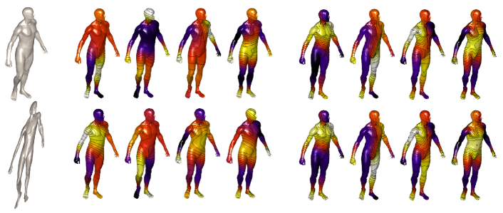
Figure 2: Four eigenfunctions of the standard (second through fifth columns) and the proposed equi-affine-invariant (four rightmost columns) Laplace-Beltrami operators. Two rows show a shape and its equi-affine transformation. For convenience of visualization, eigenfunctions are overlaid onto the untransformed shape.

5.1 Shape retrieval

Sun et al. [23] proposed using the diagonal of the heat kernel, $h_{t}(x,x)$, as a local descriptor of the shape, referred to as the heat kernel signature (HKS). In practice, the descriptor is computed by sampling the time parameter $t$ at a discrete set of points, $t_{1},\ldots,t_{n}$, and collecting the corresponding values of $h_{t}(x,x)$ into a vector $\mathbf{p}(x)=(h_{t_{1}}(x,x),\ldots,h_{t_{n}}(x,x))$. The HKS descriptor is isometry-invariant, easy to compute, and is provably informative [23]. The affine-invariant HKS descriptors can be used in one-to-one feature-based shape matching methods [23], or in large-scale shape retrieval applications using the bags of features paradigm [17]. In the latter, the shape is considered as a collection of “geometric words” from a fixed “vocabulary” and is described by the statistical distribution of such words. The vocabulary is constructed off-line by clustering the descriptor space. Then, for each point on the shape, the descriptor is replaced by the nearest vocabulary word by means of vector quantization. Counting the frequency of each word, a bag of features is constructed. The similarity of two shapes is then computed as the distance between the corresponding bags of features.

To evaluate the performance of the proposed approach for the construction of local descriptors, we used the Shape Google framework [17] based on standard and equi-affine-invariant HKS. Both descriptors were computed at six scales ($t=1024,1351.2,1782.9,2352.5$, and $4096$). Bags of features were computed using soft vector quantization with variance taken as twice the median of all distances between cluster centers in a vocabulary of $64$ entries. Approximate nearest neighbor method [2] was used for vector quantization. Both the standard and the affine-invariant Laplace-Beltrami operator discretization were computed using finite elements. Heat kernels were approximated using the first smallest $100$ eigenpairs.

Evaluation was performed using the SHREC 2010 robust large-scale shape retrieval benchmark methodology. The dataset consisted of two parts: 793 shapes from 13 shape classes with simulated transformation of different types (Figure 4) and strengths (60 per shape) used as queries, and the remaining 521 shapes used as the queried corpus. Transformations classes affine and isometry+affine were added to the original SHREC query set, representing, respectively, equi-affine transformations of different strengths of the null shape and its approximate isometry. The combined dataset consisted of 1314 shapes. Retrieval was performed by matching 780 transformed queries to the 534 null shapes. Each query had one correct corresponding null shape in the dataset. Performance was evaluated using precision/recall characteristic. Precision $P(r)$ is defined as the percentage of relevant shapes in the first $r$ top-ranked retrieved shapes. Mean average precision (mAP), defined as $mAP=\sum_{r}P(r)\cdot rel(r)$, where $rel(r)$ is the relevance of a given rank, was used as a single measure of performance. Intuitively, mAP is interpreted as the area below the precision-recall curve. Ideal retrieval performance (mAP=100%) is achieved when all queries return relevant first matches. Performance results were broken down according to transformation class and strength.

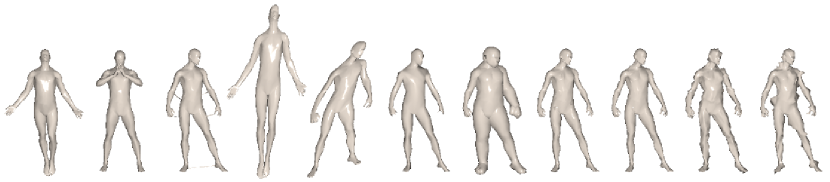
Figure 4: Examples of query shape transformations used in the shape retrieval experiment (left to right): null, isometry, topology, affine, affine+isometry, sampling, local scale, holes, microholes, Gaussian noise, shot noise.

Tables 1–2 show that the equi-affine version of the ShapeGoogle approach obtains slightly higher precision than the original ShapeGoogle in all SHREC’10 transformations. We attribute this phenomenon to the smoothing effect of the second order interpolation. In addition, equi-affine ShapeGoogle exhibits nearly perfect retrieval under equi-affine transformations in affine transformations, where the original approach fails.

	Strength
Transform.	1	$\leq$2	$\leq$3	$\leq$4	$\leq$5
Isometry	100.00	100.00	100.00	100.00	99.23
Affine	100.00	100.00	100.00	100.00	97.44
Iso.+Affine	100.00	100.00	100.00	100.00	100.00
Topology	96.15	94.23	91.88	89.74	86.79
Holes	100.00	100.00	100.00	100.00	100.00
Micro holes	100.00	100.00	100.00	100.00	100.00
Local scale	100.00	100.00	94.74	82.39	73.97
Sampling	100.00	100.00	100.00	96.79	86.10
Noise	100.00	100.00	89.83	78.53	69.22
Shot noise	100.00	100.00	100.00	97.76	89.63

Table 1: Performance (mAP in %) of Shape Google with equi-affine-invariant HKS descriptors.

	Strength
Transform.	1	$\leq$2	$\leq$3	$\leq$4	$\leq$5
Isometry	100.00	100.00	100.00	100.00	100.00
Affine	100.00	86.89	73.50	57.66	46.64
Iso.+Affine	94.23	86.35	76.84	70.76	65.36
Topology	100.00	100.00	98.72	98.08	97.69
Holes	100.00	96.15	92.82	88.51	82.74
Micro holes	100.00	100.00	100.00	100.00	100.00
Local scale	100.00	100.00	97.44	87.88	78.78
Sampling	100.00	100.00	100.00	96.25	91.43
Noise	100.00	100.00	100.00	99.04	99.23
Shot noise	100.00	100.00	100.00	98.46	98.77

Table 2: Performance (mAP in %) of Shape Google with HKS descriptors.

5.2 Global structures

The equi-affine-invariant Laplacian can also be employed in the construction of global geometric structures. By plugging it into (5), a family of equi-affine-invariant diffusion distances is obtained. Similarly, a truly affine-invariant version of the commute time metric is obtained by using the equi-affine-invariant operator in (6). These metric structures can be used in the Gromov-Hausdorff framework [10, 14], in which shapes are modeled as metric spaces, and the similarity of two shapes $(X,d_{X})$ and $(Y,d_{Y})$ is established by looking at the minimum-distortion correspondence between them. A correspondence is defined as a subset $\mathcal{C}\subset X\times Y$ such that for all $x\in X$ there exists $y\in Y$ such that $(x,y)\in\mathcal{C}$, and vice versa, for all $y\in Y$ there exists $x\in X$ such that $(x,y)\in\mathcal{C}$. The distortion of $\mathcal{C}$ is defined as

$$\mathrm{dis}(\mathcal{C}) = \max_{(x,y),(y,y^{\prime})\in\mathcal{C}}|d_{X}(x,x^{\prime})-d_{Y}(y,y^{\prime})|.$$ (13)

The Gromov-Hausdorff distance is given as the minimum of the distortion over all possible correspondences,

$$d_{\mathrm{GH}}(X,Y) = \frac{1}{2}\min_{\mathcal{C}}\mathrm{dis}(\mathcal{C}),$$ (14)

and serves as a criterion for shape similarity in the sense that two shapes with $d_{\mathrm{GH}}(X,Y)\leq\epsilon$ are at most $2\epsilon$-isometric, and, vice versa, two $\epsilon$-isometric shapes have at most $d_{\mathrm{GH}}(X,Y)\leq 2\epsilon$. A byproduct of this problem is the minimum-distortion correspondence $\mathcal{C}$.

Figure 5 shows the correspondences obtained between an equi-affine transformation of a shape using the standard and the equi-affine-invariant versions of the diffusion metric. Minimization of a least-squares version of (14) was performed using the generalized multidimensional scaling (GMDS) algorithm. In the case of the standard diffusion metric, the embedding distortion grew by over $6$ times as the result of the transformation, while in the case of the proposed invariant diffusion metric, the increase was by mere $16\%$.

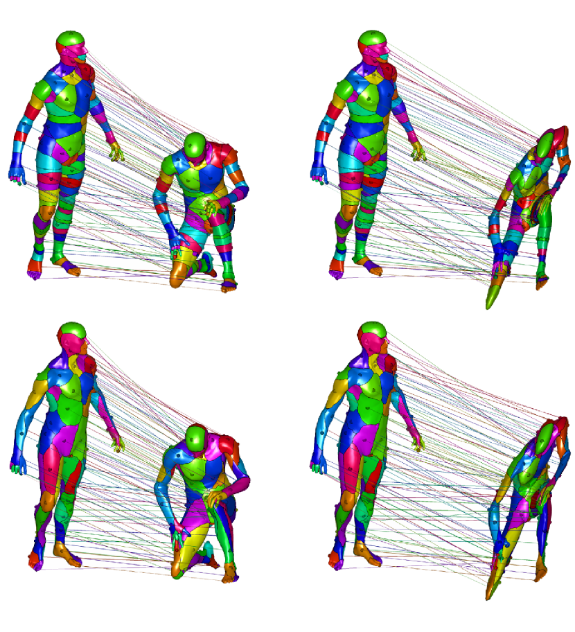
Figure 5: The GMDS framework is used to calculate correspondence between a shape and its isometry (left) and isometry followed by an equi-affine transformation (right). Matches between shapes are depicted as identically colored Voronoi cells. Standard diffusion distance (first row) and its equi-affine-invariant counterpart (second row) are used as the metric structure in the GMDS algorithm. Inaccuracies obtained in the first case are especially visible in the abdominal region.

5.3 Intrinsic symmetry detection

Ovsjanikov et al. [18] proposed detecting intrinsic symmetries of a shape by analyzing the eigenfunctions of the Laplace-Beltrami operator. Intrinsic symmetry is manifested in the existence of a self-isometry $f:X\rightarrow X$, under which the metric structure of the shape is preserved, i.e., $d=d\circ(f\times f)$, where $d$ is the commute time metric. Ovsjanikov et al. [18] observe that for any intrinsic reflection symmetry $f$, simple eigenfunctions of $\Delta$ satisfy $\phi_{i}\circ f=\pm\phi_{i}$. Thus, the symmetries of $X$ can be parameterized by the sign signature $(s_{1},s_{2},\ldots)$; $s_{i}\in\{-1,1\}$ such that $\phi_{i}\circ f=s_{i}\phi_{i}$.

Given a truncated sign signature $(s_{1},\ldots,s_{K})$, define an energy

$$E(s_{1},\ldots,s_{K})=\int\min_{x^{\prime}\in X}\sum_{i=1}^{K}\frac{1}{\lambda_{i}}(s_{i}\phi_{i}(x)-\phi_{i}(x^{\prime}))^{2}da.$$

It is easy to show that $E=0$ for sign signatures corresponding to intrinsic symmetries, and $E\approx 0$ for approximate symmetries satisfying $d\approx d\circ(f\times f)$. The symmetry itself is recovered as

$$f(x) = \mathop{\mathrm{argmin}}_{x^{\prime}\in X}\sum_{i=1}^{K}\frac{1}{\lambda_{i}}(s_{i}\phi_{i}(x)-\phi_{i}(x^{\prime}))^{2}.$$

Employing our equi-affine-invariant Laplacian, the detection of intrinsic symmetries can be made under affine transformations of the shape.

Figure 6 shows an example of intrinsic symmetry detection with the method of [18] using standard (first row) and the proposed affine-invariant (second row) Laplace-Beltrami operator on an intrinsically symmetric centaur shape that underwent a mild isometric and affine transformation. In this experiment, we use the five first non-trivial eigenfunctions and show the approximate symmetries corresponding to the sign signatures producing the smallest values of $E$ (sign signature $+++++$ corresponding to the identity transformation was ignored). While no meaningful symmetries are detected in the first case, using our affine-invariant Laplace-Beltrami operator we were able to detect three approximate symmetries of the shape: hands and forward legs reflection (left), rear legs reflection (center), and full body reflection (right).

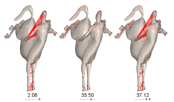
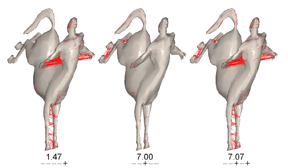
Figure 6: Symmetry detection with the method of [18] using standard (first row) and the proposed affine-invariant (second row) Laplace-Beltrami operator. Red lines depict the point correspondence $f$. For each sign signature, the corresponding error $E$ is shown.

6 Conclusions

We introduced an equi-affine-invariant Laplace-Beltrami operator on two-dimensional surfaces, and showed that it can be utilized to construct affine-invariant local and global diffusion geometric structures. Performance of the proposed tools was demonstrated on shape retrieval, correspondence, and symmetry detection applications. Our results show that affine-invariant diffusion geometries gracefully compete with, and sometimes even outperform, their classical counterparts under isometric changes and in the presence of geometric and topological noise, while significantly outperforming the latter under affine transformations.

Extension of the proposed equi-affine framework into fully affine invariance (including scale) could be accomplished by either exploiting the scale invariance property of the commute time distance, or the consideration of scale invariant signatures, two approaches we plan to study in the future.

7 Acknowledgements

This research was supported in part by The Israel Science Foundation (ISF) grant number 623/08, and by the USA Office of Naval Research (ONR) grant.

References

- [1] L. Alveraz, F. Guichard, P. L. Lions, and J. M. Morel. Axioms and fundamental equations of image processing. Archive for Rational Mechanics and Analysis, 123(3):199–257, 1993.
- [2] S. Arya, D. M. Mount, N. S. Netanyahu, R. Silverman, and A. Y. Wu. An optimal algorithm for approximate nearest neighbor searching. J. ACM, 45:891–923, 1998.
- [3] P. Bérard, G. Besson, and S. Gallot. Embedding riemannian manifolds by their heat kernel. Geometric and Functional Analysis, 4(4):373–398, 1994.
- [4] A. M. Bruckstein and D. Shaked. On projective invariant smoothing and evolutions of planarcurves and polygons. Journal of Mathematical Imaging and Vision, 7:225–240, June 1997.
- [5] S. Buchin. Affine differential geometry. Beijing, China: Science Press, 1983.
- [6] V. Caselles and C. Sbert. What is the best causal scale space for 3d images? SIAM Journal Applied Math., (56):1196–1246, 1996.
- [7] R. R. Coifman and S. Lafon. Diffusion maps. Applied and Computational Harmonic Analysis, 21:5–30, July 2006.
- [8] G. Dziuk. Finite elements for the Beltrami operator on arbitrary surfaces. In S. Hildebrandt and R. Leis, editors, Partial differential equations and calculus of variations, pages 142–155. 1988.
- [9] D. Ghosh, N. Amenta, and M. Kazhdan. Closed-form blending of local symmetries. In Proc. SGP, 2010.
- [10] M. Gromov. Structures Métriques Pour les Variétés Riemanniennes. Number 1 in Textes Mathématiques. 1981.
- [11] B. Lévy. Laplace-Beltrami eigenfunctions towards an algorithm that “understands” geometry. In Proc. Shape Modeling and Applications, 2006.
- [12] M. Mahmoudi and G. Sapiro. Three-dimensional point cloud recognition via distributions of geometric distances. Graphical Models, 71(1):22–31, January 2009.
- [13] D. Mateus, R. P. Horaud, D. Knossow, F. Cuzzolin, and E. Boyer. Articulated shape matching using laplacian eigenfunctions and unsupervised point registration. Proc. CVPR, June 2008.
- [14] F. Mémoli and G. Sapiro. A theoretical and computational framework for isometry invariant recognition of point cloud data. Foundations of Computational Mathematics, 5:313–346, 2005.
- [15] K. Mikolajczyk, T. Tuytelaars, C. Schmid, A. Zisserman, J. Matas, F. Schaffalitzky, T. Kadir, and L. V. Gool. A comparison of affine region detectors. IJCV, 65(1–2):43–72, 2005.
- [16] P. Olver, G. Sapiro, and A. Tennenbaum. Invariant geometric evolutions of surfaces and volumetric smoothing. SIAM Journal Applied Math., (57):176–194, 1997.
- [17] M. Ovsjanikov, A. M. Bronstein, M. M. Bronstein, and L. J. Guibas. Shape Google: a computer vision approach to invariant shape retrieval. In Proc. NORDIA, 2009.
- [18] M. Ovsjanikov, J. Sun, and L. J. Guibas. Global intrinsic symmetries of shapes. In Computer Graphics Forum, volume 27, pages 1341–1348, 2008.
- [19] M. Reuter, S. Biasotti, D. Giorgi, G. Patanè, and M. Spagnuolo. Discrete Laplace–Beltrami operators for shape analysis and segmentation. Computers & Graphics, 33(3):381–390, 2009.
- [20] M. Reuter, F.-E. Wolter, and N. Peinecke. Laplace-spectra as fingerprints for shape matching. In Proc. ACM Symp. Solid and Physical Modeling, pages 101–106, 2005.
- [21] R. M. Rustamov. Laplace-Beltrami eigenfunctions for deformation invariant shape representation. In Proc. SGP, pages 225–233, 2007.
- [22] N. Sochen. Affine-invariant flows in the Beltrami framework. Journal of Mathematical Imaging and Vision, 20(1):133–146, 2004.
- [23] J. Sun, M. Ovsjanikov, and L. J. Guibas. A concise and provably informative multi-scale signature based on heat diffusion. In Proc. SGP, 2009.