Linear and nonlinear Stark effect in triangular molecule

Abstract

We analyze changes of the electronic structure of a triangular molecule under the influence of an electric field (i.e., the Stark effect). The effects of the field are shown to be anisotropic and include both a linear and a nonlinear part. For strong electron correlations, we explicitly derive exchange couplings in an effective spin Hamiltonian. For some conditions one can find a dark spin state, for which one of the spins is decoupled from the others. The model is also applied for studying electronic transport through a system of three coherently coupled quantum dots. Since electron transfer rates are anisotropic, the current characteristics are anisotropic as well, differing for small and large electric field.

I Introduction

In this paper we investigate electronic properties of a model of a triangular molecule in a presence of an electric field. Recently, similar models were considered for systems of three coherently coupled quantum dots (QDs), Gardreau2006 ; Delgado2008 ; Busl ; Brandes ; Emary ; Poltl ; Kostyrko09 ; Zitko , for magnetic interactions in molecules,gatteschi ; choi ; trif ; tsukerblatt as well as for complex phase orderings in strongly correlated electronic materials with a triangular lattice (e.g., multiferroics bulaevskii , cobaltates cobaltates , or organic compounds powell ). These simple models exhibit plenty of interesting physics. For example, in the system of quantum dots, one finds complex charge and spin arrangementsGardreau2006 , which can be classified according a set of topological Hund s rules. For some interference conditions a so-called dark state can occur, for which one of the QDs is decoupled from the reservoirs and an electron can be trapped.Brandes Consequently, electronic transport is changed; one can observe a rectification effect, negative differential resistance, and an enhancement of the shot noise.Emary Moreover, one can expect the Aharonov-Bohm effect, when a magnetic flux penetrates the triangle. Moreover, one can expect theAharonov-Bohm effect, when a magnetic flux penetrates the triangle. The effect leads to a crossover from the singlet to the triplet ground state, which manifests itself in spin blockade in transport Delgado2008 and interesting spin dynamics under two-electron-spin-resonance Busl . For the regime of coherent transport one can expect the very rich phase diagram with many types of the Kondo resonances Zitko .

Our studies concern the Stark effect in the system of strongly correlated electrons and they are addressed mainly to coherently coupled quantum dots. For a small number of electrons ($n=1$ and $n=2$ in the triangle) the electric field induces a large polarization, and many aspects were already considered Gardreau2006 ; Delgado2008 ; Busl ; Brandes ; Emary ; Poltl ; Kostyrko09 ; Zitko . In this paper we focus on the situation with $n=3$ electrons, for which the induced polarization is minor, because the Coulomb interactions dominate and hinder a possible shift of an electronic charge. First we will show that the electric field leads to splitting of energy levels as well as to breaking of the symmetry of the system and changes the symmetry of wave functions. We demonstrate that the electric field can induce significant changes in a spin arrangement. It also results in changes of coupling between spins and different characteristics of spin-spin correlation functions with respect to an angle the electric field forms with the median of the triangle. In particular we will show conditions for the appearance of the dark spin state. Second we will show how the Stark effect manifests itself in electronic transport. We confine ourselves to the case in which at equilibrium the ground state is singlet or triplet and for an applied bias voltage excited states with three electrons (doublets and quadruplets) participate in transport.

II Influence of electric field on spin states

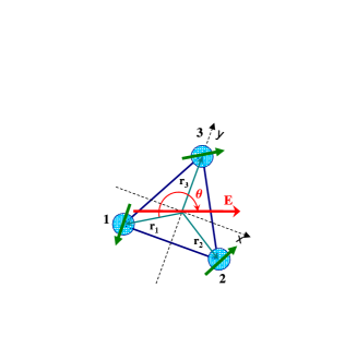
Figure 1: (Color online) The considered model of a triangular molecule placed in an electric field $\mathbf{E}$.

A model of a triangular molecule in the presence of an electric field $\mathbf{E}$ is shown in Fig.1. The corresponding Hamiltonian can be expressed as

$$H_{M}=t\sum_{i<j,\sigma}(c^{\dagger}_{i\sigma}c_{j\sigma}+h.c.)+U_{0}\sum_{i}n_{i\uparrow}n_{i\downarrow}$$

$$+U_{1}\sum_{i<j,\sigma,\sigma^{\prime}}n_{i\sigma}n_{j\sigma^{\prime}}+Eer\sum_{i,\sigma}\cos[(\theta+(i-1)\frac{2\pi}{3}]\,n_{i\sigma},$$ (1)

where the first term describes electron hopping between nearest neighbor sites. For the sake of generality we consider $t<0$ as well as $t>0$, for which the model describes the system of QDs with electrons or holes, respectively. The second and the third terms correspond to insite and intersite Coulomb interactions. The last term takes into account the influence of the electric field $\mathbf{E}$ on the electronic polarization $\hat{\mathbf{P}}=e\sum_{i,\sigma}\mathbf{r}_{i}n_{i\sigma}$, where $\mathbf{r}_{i}$ denotes the vector pointing to the site $i$, $e$ - a charge of an electron, $\theta$ - the angle between $\mathbf{r}_{1}$ and $\mathbf{E}$, $d$ - the length of the arm of the triangle and $r=d/\sqrt{3}$. One can see that the electric field modulates the local site energies: $\epsilon_{i}=g_{E}\cos[\theta+(i-1)2\pi/3]$. In further considerations we take $g_{E}=Eer$ as a coupling parameter.

For $n=3$ electrons in the system the wave functions are constructed from the singlet and the triplet states by adding an electron (see [pauncz, ]). There are quadruplet states (^3/2Q${}_{S_{z}}$) with $S=3/2$, $S_{z}=\pm 3/2$, $\pm 1/2$, and the corresponding wave functions are constructed from the triplet states by adding an electron. The ground state is, however, the doublet state (^1/2D${}_{S_{z}}$) with $S=1/2$, $S_{z}=\pm 1/2$, which can be formed from the states

$$|\text{D}_{S_{z}}\rangle_{1}=\frac{1}{\sqrt{2}}c^{\dagger}_{1\sigma}(c^{\dagger}_{2\sigma}c^{\dagger}_{3\overline{\sigma}}-c^{\dagger}_{2\overline{\sigma}}c^{\dagger}_{3\sigma})\left|\mathrm{vac}\right\rangle,$$ (2)

$$|\text{D}_{S_{z}}\rangle_{2}=\frac{1}{\sqrt{6}}[2\;c^{\dagger}_{1\overline{\sigma}}c^{\dagger}_{2\sigma}c^{\dagger}_{3\sigma}-c^{\dagger}_{1\sigma}(c^{\dagger}_{2\sigma}c^{\dagger}_{3\overline{\sigma}}+c^{\dagger}_{2\overline{\sigma}}c^{\dagger}_{3\sigma})]\left|\mathrm{vac}\right\rangle$$ (3)

and the states with double site occupancy $c^{\dagger}_{1\sigma}c^{\dagger}_{1\overline{\sigma}}c^{\dagger}_{2\sigma}\left|\mathrm{vac}\right\rangle$, $c^{\dagger}_{2\sigma}c^{\dagger}_{2\overline{\sigma}}c^{\dagger}_{3\sigma}\left|\mathrm{vac}\right\rangle$, etc. The function $|\text{D}_{S_{z}}\rangle_{1}$ and $|\text{D}_{S_{z}}\rangle_{2}$ are constructed respectively from the singlet and the triplet state at the 23–bond by adding an electron to the QD 1.

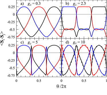
Figure 2: (Color online) Expectation values of the spin correlators $\mathbf{S}_{1}\cdot\mathbf{S}_{2}$, $\mathbf{S}_{2}\cdot\mathbf{S}_{3}$ and $\mathbf{S}_{3}\cdot\mathbf{S}_{1}$ (black, red and blue curves, respectively) calculated for the ground state as a function of the angle $\theta$ of the electric field with respect to the triangle. The plots are obtained for the Hubbard model (1) with a large $U_{0}=30$, $U_{1}=2$, $t=1$, $g_{E}=0.3$ (a), $g_{E}=2.5$ (b), $g_{E}=5$ (c) and $g_{E}=10$ (d). For comparison the dashed curves represent the spin correlators for the Heisenberg model (4) with the modulated exchange couplings $J_{ij}$ given by Eq.(5) – [for smaller $g_{E}\leq 5$ the dashed curves cover the solid ones within the plot resolution].

Fig.2 presents an evolution of the spin-spin correlation functions when the electric field increases, it manifests a transition from the linear to the quadratic Stark effect. For small fields the spin-correlation functions oscillate with the period $2\pi$. At an intermediate value $|g_{E}|=4|t|$ a crossover occurs, and for a larger $g$ the functions $\langle\mathbf{S}_{i}\cdot\mathbf{S}_{j}\rangle$ show new components due to the quadratic Stark effect. One can see in Fig.2a and 2b that at $\theta=0$ (where the electric field is perpendicular to the 23-bond and points to the 1-st site) the spin correlators $\langle\mathbf{S}_{1}\cdot\mathbf{S}_{2}\rangle=\langle\mathbf{S}_{3}\cdot\mathbf{S}_{1}\rangle=0$ and $\langle\mathbf{S}_{2}\cdot\mathbf{S}_{3}\rangle\approx-0.75$. This means that the spin at QD1 is uncoupled from the spins forming the singlet at the 23-bond, and the corresponding state is $|\text{D}_{S_{z}}\rangle_{1}$. We call such a configuration the dark spin state, in contrast to the dark states for $n=1$ and $n=2$ electrons in the triangle molecule, when their properties are connected to a specific charge distribution.Brandes ; Emary With rotation of the electric field, the dark spin state occurs at $\theta=2\pi/3$ ($\theta=4\pi/3$), when the uncoupled spin is located at the QD 2 (3) and the singlet state is at the 12 (31) bond (the electric field is then perpendicular to the bond). The situation is more complex for a large $|g_{E}|>4|t|$, when the quadratic Stark effect begins to dominate and gradually changes the period of oscillation of $\langle\mathbf{S}_{i}\cdot\mathbf{S}_{j}\rangle$ as well as the configuration of the dark spin states.

In order to understand the crossover from small to large fields, we perform the perturbative canonical transformation of the Hubbard Hamiltonian (1) to an effective Heisenberg Hamiltonian, treating the intersite terms (both the hopping and the intersite Coulomb interaction terms) as small ones.macdonald To take into account both the linear and non-linear Stark effect the perturbation expansion should be carried out to the third order (see the Appendix for details). For $n=3$ electrons the effective Hamiltonian reads

$$\tilde{H} = 3U_{1}+\sum_{i<j}J_{ij}\left(\vec{S}_{i}\cdot\vec{S}_{j}-\frac{1}{4}\right)\,,$$ (4)

with the exchange coupling

$$J_{ij}=\frac{4t^{2}}{U_{0}}+\frac{4t^{2}(\epsilon_{j}-\epsilon_{i})^{2}}{U_{0}^{3}}+\frac{8t^{3}(2\epsilon_{m}-\epsilon_{i}-\epsilon_{j})}{U_{0}^{3}}\,,$$ (5)

where the indices $i,j,m$ denote three different sites. Here, we also assumed that the on-site Coulomb interactions are stronger than the electric field, i.e. $U_{0}\gg{}\epsilon_{i}$. It is seen that for the weak field the third order term [the third term in Eq.(5)] depends linearly on the electric field $E$, whereas the second order term behaves like a second power of $E$ and its period of oscillations is twice as large as the linear term. This result presents one of the main differences between the Stark effect in the system of strongly correlated electrons and that in atomic physics friedrich .

For a very large $g_{E}$, when the quadratic term dominates, the dark spin state can occur for $\mathbf{E}$ parallel to a bond of the triangle. Then the singlet state is formed on this bond and the uncoupled spin is at the opposite QD. In this limit there is a direct exchange process, which is symmetric with respect to exchange of spins between QDs, and it does not depend on the orientation of the dipole (it is a quadratic dependence on $E$). Since the exchange coupling $J_{ij}$ depends on the difference of site energies [see Eq.(5)], its maximal value is at the electric field parallel to the bond. For this case two other exchange couplings are equal, and the dark spin state appears.

Figure 3: (Color online) Splitting of states by the electric field in the effective Heisenberg model (4). The solid curves represent the states $E_{\text{D}1}$ and $E_{\text{D}2}$ for $\theta=0$, whereas the dashed curves represent $E_{\text{D}1^{\prime}}$, $E_{\text{D}2^{\prime}}$ for $\theta=\pi/3$ ($t=1$, $U_{0}=30$, $U_{1}=2$).

The eigenvalues of the Hamiltonian (4) can be readily obtained as

$$E_{\text{Q}}=3U_{1},$$ (6)

$$E_{\text{D}1,2}=3U_{1}-(6J\pm 2\Delta)/4$$ (7)

for quadruplet and doublet, respectively. Here, $J=(J_{12}+J_{23}+J_{31})/3$ and $\Delta=\sqrt{J_{12}^{2}+J_{23}^{2}+J_{31}^{2}-J_{12}J_{23}-J_{12}J_{31}-J_{23}J_{31}}$. If the electric field is perpendicular to the $ij$-bond, $\epsilon_{i}=\epsilon_{j}$, the exchange couplings $J_{im}=J_{jm}$ and we have the dark spin state. In particular for $\theta=0$, $J_{12}=J_{31}$ and the eigenvalues are

$$E_{\text{D}1}=3U_{1}-\frac{3J}{4}-J_{23},$$ (8)

$$E_{\text{D}2}=3U_{1}-\frac{3J}{4}-J_{12},$$ (9)

for which the corresponding wavefunctions are: $|\text{D}_{S_{z}}\rangle_{1}$ and $|\text{D}_{S_{z}}\rangle_{2}$ [given by Eq.(2) and (3)], respectively. Fig.3 presents the plot of these eigenenergies as a function of the electric field. In this case $|\text{D}_{S_{z}}\rangle_{1}$ is the dark spin state, but its energy $E_{\text{D}1}<E_{\text{D}2}$ for $g_{E}<4t$ only. Fig.3 also shows the eigenergies $E_{\text{D}1^{\prime}}$ and $E_{\text{D}2^{\prime}}$ for the case $\theta=\pi/3$ (when the electric field is perpendicular to the 13 bond and its direction is opposite to the 2-nd site). Now the corresponding eigenstates are

$$|\text{D}_{S_{z}}\rangle_{1^{\prime}}=\frac{1}{\sqrt{2}}\;c^{\dagger}_{2\sigma}(c^{\dagger}_{3\sigma}c^{\dagger}_{1\overline{\sigma}}-c^{\dagger}_{3\overline{\sigma}}c^{\dagger}_{1\sigma})|\mathrm{vac}\rangle,$$ (10)

$$|\text{D}_{S_{z}}\rangle_{2^{\prime}}=\frac{1}{\sqrt{6}}\;[2c^{\dagger}_{2\overline{\sigma}}c^{\dagger}_{3\sigma}c^{\dagger}_{1\sigma}-c^{\dagger}_{2\sigma}(c^{\dagger}_{3\sigma}c^{\dagger}_{1\overline{\sigma}}+c^{\dagger}_{3\overline{\sigma}}c^{\dagger}_{1\sigma})]|\mathrm{vac}\rangle.$$ (11)

However in this case the dark spin state $|\text{D}_{S_{z}}\rangle_{1^{\prime}}$ is the excited state ($E_{\text{D}1^{\prime}}>E_{\text{D}2^{\prime}}$). In the both presented cases the states $|\text{D}_{S_{z}}\rangle_{1}$, $|\text{D}_{S_{z}}\rangle_{1^{\prime}}$ are constructed from the singlet states, whereas $|\text{D}_{S_{z}}\rangle_{2}$, $|\text{D}_{S_{z}}\rangle_{2^{\prime}}$ are constructed from the triplet states.

III Transport in sequential tunneling regime

Let us now analyze electronic transport in a sequential tunneling regime through our system with the left and the right electrode connected to the QD 1 and 2, respectively. In our calculations we need transfer rates from the L (R) electrode to the molecule Weinmann95

$$\Gamma^{L(R)+}_{\nu_{2}\to{}\nu_{3}}=\gamma_{L(R)}\,\sum_{\sigma}|\langle\nu_{3}|c^{\dagger}_{1(2)\sigma}|\nu_{2}\rangle|^{2}f(\Delta E_{\nu_{2}\nu_{3}}-\mu_{L(R)}),$$

where $|\nu_{n}\rangle$ denotes the initial state for $n$ electrons, $\Delta E_{\nu_{2}\nu_{3}}=E_{\nu_{3}}-E_{\nu_{2}}$ is the corresponding energy difference, $\gamma_{L(R)}$ is a net transfer rate through the potential barier between the electrode and the molecule, $f$ denotes the Fermi distribution function, the chemical potentials are taken as $\mu_{L}=E_{F}$, $\mu_{R}=E_{F}+eV$, $E_{F}$ is the Fermi energy and $V$ is a bias voltage. Similarly, one can write $\Gamma^{L(R)-}_{\nu_{3}\to{}\nu_{2}}$ for the reverse tunneling process when the electron leaves the molecule.

Since the quadruplet functions $|{\mathrm{Q}}_{S_{z}}\rangle$ are constructed from the triplets $|\text{T}_{S_{z}}\rangle$, therefore, the nonzero transfer matrix elements are only:

$$|\langle{\mathrm{Q}}_{\pm 3/2}|c^{\dagger}_{1(2)\sigma}|{\mathrm{T}}_{\pm 1}\rangle|=\sqrt{2}\;|\langle{\mathrm{Q}}_{\pm 1/2}|c^{\dagger}_{1(2)\sigma}|{\mathrm{T}}_{0}\rangle|$$

$$=\sqrt{3}\;|\langle{\mathrm{Q}}_{\pm 1/2}|c^{\dagger}_{1(2)\overline{\sigma}}|{\mathrm{T}}_{\pm 1}\rangle|=|x^{T}_{2(1)3}|\,$$ (13)

for $\sigma=\pm 1/2$. Here, we use $|{\mathrm{T}}_{S_{z}}\rangle$ (the singlet solution $|\text{S}\rangle$) as a linear combination of triplets (singlets) localized on the $ij$ bonds, and $x^{T}_{ij}$ ($x^{S}_{ij}$) denote the corresponding coefficients. The doublet wavefunction is a linear combination of $|\text{D}_{S_{z}}\rangle_{1}$ and $|\text{D}_{S_{z}}\rangle_{2}$ [with the coefficient $x^{D}_{1}$ and $x^{D}_{2}$] as well as the states with double site occupancy. We have checked that for a large $U_{0}$ the transfer matrix elements for the states with double occupied sites play a minor role in electronic transport, and thus they are ignored. The corresponding elements are:

$$|\langle{\mathrm{D}}_{\pm 1/2}|c^{\dagger}_{1\overline{\sigma}}|{\mathrm{T}}_{\pm 1}\rangle|=\sqrt{2}\;|\langle{\mathrm{D}}_{\pm 1/2}|c^{\dagger}_{1\sigma}|{\mathrm{T}}_{0}\rangle|$$

$$\approx\sqrt{2/3}\;|x^{D}_{2}x^{T}_{23}|,$$ (14)

$$|\langle{\mathrm{D}}_{\pm 1/2}|c^{\dagger}_{2\overline{\sigma}}|{\mathrm{T}}_{\pm 1}\rangle|=\sqrt{2}\;|\langle{\mathrm{D}}_{\pm 1/2}|c^{\dagger}_{2\sigma}|{\mathrm{T}}_{0}\rangle|$$

$$\approx|(x^{D}_{1}/\sqrt{2}+x^{D}_{2}/\sqrt{6})x^{T}_{13}|,$$ (15)

$$|\langle{\mathrm{D}}_{\pm 1/2}|c^{\dagger}_{1\sigma}|{\mathrm{S}}\rangle|\approx|x^{D}_{1}x^{S}_{23}|,$$ (16)

$$|\langle{\mathrm{D}}_{\pm 1/2}|c^{\dagger}_{2\sigma}|{\mathrm{S}}\rangle|\approx 1/2|(x^{D}_{1}-\sqrt{3}x^{D}_{2})x^{S}_{13}|.$$ (17)

Next, we solve the corresponding master equation Weinmann95

$$\frac{dP_{\nu_{n}}}{dt} = \sum_{\ell,\nu_{n-1}}\Gamma^{\ell+}_{\nu_{n-1}\to{}\nu_{n}}P_{\nu_{n-1}}+\sum_{\ell,\nu_{n+1}}\Gamma^{\ell-}_{\nu_{n+1}\to{}\nu_{n}}P_{\nu_{n+1}}$$ (18)

$$- P_{\nu_{n}}(\sum_{\ell,\nu_{n-1}}\Gamma^{\ell-}_{\nu_{n}\to{}\nu_{n-1}}+\sum_{\ell,\nu_{n+1}}\Gamma^{\ell+}_{\nu_{n}\to{}\nu_{n+1}})$$

to find the occupation probability $P_{\nu_{n}}$ of the eigenstates $|\nu_{n}\rangle$ in the steady limit, i.e. for $dP_{\nu_{n}}/dt=0$. The current in this limit reads

$$I=e\sum_{\nu_{2},\nu_{3}}\left(\Gamma^{L+}_{\nu_{2}\to{}\nu_{3}}P_{\nu_{2}}-\Gamma^{L-}_{\nu_{3}\to{}\nu_{2}}P_{\nu_{3}}\right).$$ (19)

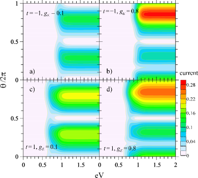
Figure 4: (Color online) Maps of the current as a function of the bias voltage $V$ and the angle $\theta$ of the electric field with respect to the triangle for $g_{E}=0.1$ (left column) and $g_{E}=0.8$ (right column). The Fermi level is taken $E_{F}=5.1$, so at equilibrium the system contains two electrons in the singlet (triplet) state for $t=-1$ ($t=1$) - top (bottom) plots, respectively. We also assumed that $U_{0}=30$, $U_{1}=2$, the temperature $T=0.05$, $\gamma_{L}=\gamma_{R}=\gamma_{0}$, and the current is in units of $e\gamma_{0}$.

The results of numerical calculations are presented in Fig.4 as a map in the $V$-$\theta$ space. Here we assumed that the electric field parameter $g_{E}$ can be controlled independently of the bias voltage, e.g. by means of application of additional lateral or back gate electrodes. For small fields ($g_{E}=0.1$) one can see negative differential resistance (NDR) (an increase and next a drop of $I$ with $V$) at $\theta\approx 0$ and $\theta\approx\pi$. The NDR effect is due to charge accumulation on the dark state and the interchannel Coulomb blockade Emary . We have also analyzed all current contributions $I_{\nu_{2},\nu_{3}}$ through various energy levels. As expected the current flows via the singlet and the both doublet states for $t=-1$ (top plots in Fig.4). Although the other states are in the voltage window, they play a minor role and the corresponding $I_{\nu_{2},\nu_{3}}$ are exponentially small (these processes are thermally activated only). The situation for $g_{E}=0.8$ (Fig.4b) is different. One sees that the values of $I$ are higher and the $\theta$ dependence is different. At $\theta\approx\pi/3$ a new minimum appears. It is an evidence of the Stark effect, which is also manifested in activation of the triplet and the quadruplet states. The transfer of electrons via the quadruplet state is now substantial and its contribution $I_{\text{T,Q}}$ is larger than those from the other states. This situation can be explained by analyzing the activation energies $\Delta E_{\nu_{2},\nu_{3}}$ in Fig.5a and the corresponding transfer rates $\Gamma^{L+}_{\nu_{2}\to{}\nu_{3}}$. Since the singlet is the nondegenerate ground state, it shows the quadratic Stark effect and $\Delta E_{\text{SD}}$ is a parabola. In contrast to that the activation energies from the triplet state $\Delta E_{\text{TD}}$ and $\Delta E_{\text{TQ}}$ show, for $\theta=5\pi/3$, a linear and a parabolic dependence. For this case the triplet levels can be derived explicitly as:

$$E_{\text{T}}=U_{1}+t-\frac{g_{E}}{2},$$

$$E_{\text{T}}=U_{1}+\frac{1}{4}(g_{E}-2t\pm\sqrt{9g_{E}^{2}+12g_{E}t+36t^{2}}).$$ (20)

We took the Fermi energy as $E_{F}=5.1$, thus, for a small $g_{E}$, $\Delta E_{\text{TD}}<\Delta E_{\text{TQ}}<E_{F}$ and the corresponding transfer rates $\Gamma^{L+}_{\text{T}\to{}\text{D}}$ and $\Gamma^{L+}_{\text{T}\to{}\text{Q}}$ [see Eq.(III)] are exponentially small. For larger fields ($g_{E}>0.2$) these energies are above $E_{F}$ and the transfer rates $\Gamma^{L+}_{\text{T}\to{}\text{D}}$ and $\Gamma^{L+}_{\text{T}\to{}\text{Q}}$ are activated together with $\Gamma^{L+}_{\text{S}\to{}\text{D}}$ (the current starts to flow through all these levels at a threshold voltage).

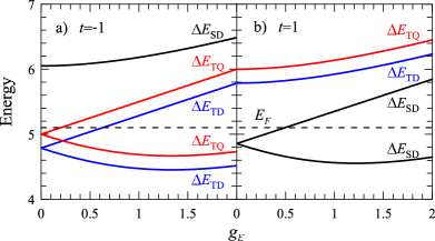
Figure 5: (Color online) Electric field dependence of the energy difference $\Delta E_{\nu_{2}\nu_{3}}$ for the most relevant states participating in electronic transport. The plots a) and b) are for the case $t=-1$ and $t=1$, which correspond to the current maps in Fig.4 for the top and the bottom panels at $\theta=5\pi/3$ and $E_{F}=5.1$, when at equilibrium the ground state is the singlet and the triplet, respectively. Here, we omit the indices 1 and 2 for the doublet states, because their activation energies are very close to each other.

The bottom row of Fig.4 presents the current maps for the case $t=1$, for which the triplet is the ground state at equilibrium. For a bias voltage larger than a threshold one (for $eV\gtrsim 0.7$), electrons are transferred via the triplet and the doublet states as well as the quadruplet state. We can clearly see (at $eV\approx 0.9$) the second step in the current, when the quadruplet state is activated. In this case, the current maps are also different for a small and large $g_{E}$. This results from the dependence of the activation energies $\Delta E_{\nu_{2},\nu_{3}}$ (and the transfer rates) on the electric field. Fig.5b shows that $\Delta E_{\text{SD}}$ (almost) linearly increases with $g_{E}$ and for large $g_{E}$ $\Delta E_{\text{SD}}>E_{F}$. Therefore, the transfer rate $\Gamma^{L+}_{\text{S}\to{}\text{D}}$ is activated.

It is worth noticing that the degenerate states (the triplet $E_{T}$ for $t=-1$ as well as the singlet $E_{S}$ for $t=1$) have different dependences on the electric field [see Eq.(III), the plots for $\Delta_{\text{TD}}$ and $\Delta_{\text{TQ}}$ in Fig.5a as well as for $\Delta_{\text{SD}}$ in Fig.5b]. One of them is linear vs $g_{E}$, whereas the second one is nonlinear. This is in contrast to the Stark effect in atomic physicsfriedrich , for which all degenerate states show a linear field dependence in a wide range.

Here we analyzed the electronic transport, in which two- and three-electron states (with transitions $|\nu_{2}\rangle\leftrightarrow|\nu_{3}\rangle$) participated. By using the electron-hole symmetry of the model (1) one obtains the same results for transitions $|\nu_{3}\rangle\leftrightarrow|\nu_{4}\rangle$ (between the states with three and four electrons) - provided that one changes the sign of the hopping $t$.

IV Conclusions

Summarizing, we considered the influence of the electric field on strongly correlated electrons in the triangular molecule (the linear and the quadratic Stark effect). The orientation $\theta$ of $\mathbf{E}$ with respect to the molecule is important, because the electric field breaks the symmetry of the system and changes the symmetry of wave functions. For some $\theta$ one finds the dark states, responsible for negative differential resistance. For $n=3$ electrons we derived the kinetic exchange coupling $J_{ij}$ between the spins, which showed quadratic and linear dependence on $\mathbf{E}$. The spin-spin correlation functions exhibit different angle $\theta$ characteristics for a small and large $\mathbf{E}$. In particular, we studied the dark spin states and their evolution with $\mathbf{E}$. The model can be applied to studies of entanglement of three spin qubits acin with the electric field in its specific role. In particular, it can be applied to a description of an experiment just recently performed in a system of three QDs, laird which presented coherent spin manipulation in a qubit with the logical basis formed from the doublet states: $|\text{D}_{S_{z}}\rangle_{1}$ and $|\text{D}_{S_{z}}\rangle_{2}$. Moreover, we predict that the anisotropic Stark effect should be seen in electronic transport.

The studied model is general and can be applied to real molecules with the triangular symmetry, to study their magnetic and optical features of interest for molecular spintronics. For example, we predict that spacial anisotropy induced by the electric field in the effective Heisenberg model will be manifested in molecular magnetism (e.g. in magnetization, magnetic susceptibility, or ESR spectra) gatteschi ; choi ; tsukerblatt . Moreover, the model can be the paradigm for materials with strongly correlated electrons on triangular lattices bulaevskii ; cobaltates ; powell . In our opinion multiferroics are the best candidates to observe the Stark effect, because in such materials local ferroelectric orderings can modify exchange couplings between spins as well as magnetic orderings.

Appendix A Canonical transformation of the Hubbard model with modulation of site energy

Here we apply a canonical perturbation theory for the Hamiltonian (II) for $U_{1}=0$, which we rewrite here as:

$$H=W+T_{0}+T_{-1}+T_{+1}$$ (21)

where $W$ represent the sum of all the single site terms, and $T_{n}$ is a contribution to the hopping part of the Hamiltonian which increases by $n$ the number of the double occupied sites in the system. Using Hubbard operatorsHubbard-64 $X_{i}^{\alpha\alpha^{\prime}}\equiv|\alpha\rangle\langle\alpha^{\prime}|$ (defined in terms of the exact eigenstates $|\alpha\rangle$ for an isolated site $i$) the contributions to the model (21) can be represented by:

$$W = \sum_{i,\alpha}E_{i\alpha}X_{i}^{\alpha\alpha}$$

$$T_{0} = \sum_{i<j,\sigma}t_{ij}(X_{i}^{\sigma 0}X_{j}^{0\sigma}+X_{i}^{2\sigma}X_{j}^{\sigma 2}),$$

$$T_{+1} = \sum_{i<j,\sigma}\sigma t_{ij}X_{i}^{2,-\sigma}X_{j}^{0\sigma},\hskip 20.00003ptT_{-1}=T^{\dagger}_{+1}$$ (22)

The site energies: $E_{i\alpha}\in\{0,\epsilon_{i},2\epsilon_{i}+U_{0}\}$ correspond to the eigenstates $\alpha\in\{0,\uparrow,\downarrow,2\}$. The following analysis is valid for a limit of the small $T_{n}$, when the differences between energies $E_{i\alpha}$ for single and double occupied sites are much larger than the hopping parameters. In the derivation of the effective Hamiltonian we apply the perturbation theory with respect to the hopping part, which can be formulated in terms of the recursive canonical transformation.macdonald With the use of the Hubbard operators the method can be easily generalized to an arbitrary form of the on–site zero–order Hamiltonian, including the site–dependent terms.maska

A.1 The effective second order spin Hamiltonian

Up to the second order with respect to the hopping part the transformed Hamiltonian reads

$$\tilde{H}=e^{-iS}He^{iS}\approx H_{0}+\frac{1}{2}[iS,H_{1}].$$ (23)

where $H_{0}=W+T_{0}$ and $H_{1}=T_{+1}+T_{-1}$. Here, it is assumed that in the expansion the linear term with respect to the off–diagonal part of hopping vanishes, which is guaranteed by a condition:

$$[iS,H_{0}]=-H_{1}.$$ (24)

From this condition we can derive in the explicit form the transformation matrix

$$iS=\sum_{i<j}iS_{ij},$$

$$iS_{ij}=\sum_{\sigma}\left(\frac{\sigma t_{ij}}{\Delta_{ij}}X_{i}^{-\sigma 2}X_{j}^{\sigma 0}-\frac{\sigma t_{ij}}{\Delta_{ji}}X_{i}^{\sigma 0}X_{j}^{-\sigma 2}\right.$$

$$\left.-\frac{\sigma t_{ij}}{\Delta_{ji}}X_{i}^{0\sigma}X_{j}^{2-\sigma}+\frac{\sigma t_{ij}}{\Delta_{ij}}X_{i}^{2-\sigma}X_{j}^{0\sigma}\right).$$ (25)

where $\Delta_{ij}=\epsilon_{i}+U_{0}-\epsilon_{j}$. After inserting the operator $S$ (A.1) into (23) we obtain the effective Hamiltonian valid up to second order perturbation with respect to the hopping part. In a form projected to the subspace $C_{00}$, defined as subspace of many-electron states with all sites singly occupied, i.e. for $n=3$ electrons in the triangle, the Hamiltonian reads:

$$\tilde{H}|_{C_{00}} = W+\frac{1}{2}\sum_{i<j,\sigma,\alpha}\sigma\alpha\,J^{(2)}_{ij}\,X_{i}^{-\sigma\alpha}X_{j}^{\sigma,-\alpha}$$ (26)

where

$$J^{(2)}_{ij}=2t_{ij}^{2}(\Delta_{ij}^{-1}+\Delta_{ji}^{-1}).$$ (27)

The effective Hamiltonian can be rewritten in a more familiar form with a help of the spin operators

$$\tilde{H}|_{C_{00}} = W+\sum_{i<j}J^{(2)}_{ij}\left(\vec{S}_{i}\cdot\vec{S}_{j}-\frac{1}{4}\right).$$ (28)

A.2 The effective third order spin Hamiltonian

A derivation of the higher order terms in a general case is based on the recursive procedure,macdonald however it is rather involved and will be discussed in a separate paper. Here we only present the extra 3rd order term projected to the $C_{00}$ subspace

$$\left.\tilde{H}^{(3)}\right|_{C_{00}} = \sum_{i<j}J^{(3)}_{ij}\left(\vec{S}_{i}\cdot\vec{S}_{j}-\frac{1}{4}\right).$$ (29)

The exchange parameter reads:

$$J^{(3)}_{ij}=2\,t_{ji}t_{im}t_{mj}\left(\Delta^{-1}_{ij}\Delta^{-1}_{im}+\Delta^{-1}_{ji}\Delta^{-1}_{jm}\right.$$

$$+\Delta^{-1}_{im}\Delta^{-1}_{jm}\left.-\Delta^{-1}_{ji}\Delta^{-1}_{mi}-\Delta^{-1}_{ij}\Delta^{-1}_{mj}-\Delta^{-1}_{mi}\Delta^{-1}_{mj}\right).$$ (30)

Here, the indices $i,j,m$ denote three different sites. Note, that the extra term vanishes for the uniform case $\epsilon_{1}=\epsilon_{2}=\epsilon_{3}$.

By expanding $J^{(2)}_{ij}$ and $J^{(3)}_{ij}$ [Eqs.(A.7) and (A.10)] in a series with respect to $\epsilon_{i}\ll U_{0}$ we ontain the exchange coupling Eq.(5).

References

- (1) L. Gaudreau, S. A. Studenikin, A. S. Sachrajda, P. Zawadzki, A. Kam, J. Lapointe, M. Korkusinski, and P. Hawrylak, Phys. Rev. Lett. 97, 036807 (2006); F. Delgado, Y.-P. Shim, M. Korkusinski, and P. Hawrylak, Phys. Rev. B 76, 115332 (2007); M. Korkusinski, I. P. Gimenez, P. Hawrylak, L. Gaudreau, S. A. Studenikin, and A. S. Sachrajda, Phys. Rev. B 75, 115301 (2007); Y.-P. Shim and P. Hawrylak, Phys. Rev. 78, 165317(2008).
- (2) F. Delgado, Y.-P. Shim, M. Korkusinski, L. Gaudreau, S. A. Studenikin, A. S. Sachrajda, and P. Hawrylak, Phys. Rev. Lett. 101, 226810 (2008).
- (3) M. Busl, R. Sánchez, and G. Platero, Phys. Rev. B 81, 121306 (2010).
- (4) T. Brandes and F. Renzoni, Phys. Rev. Lett., 85, 4148 (2000); T. Brandes, Phys. Rep. 408, 315 (2005); B. Michaelis, C. Emary and C. W. J. Beenakker, Europhys. Lett., 73, 677 (2006).
- (5) C. Emary, Phys. Rev. B 76, 245319 (2007).
- (6) C. Pöltl, C. Emary, and T. Brandes, Phys. Rev. B 80, 115313 (2009).
- (7) T. Kostyrko and B. R. Bułka, Phys. Rev. B 79, 075310 (2009).
- (8) R. Žitko and J. Bonča, Phys. Rev. B 77, 245112 (2008).
- (9) D. Gatteschi, R. Sessoli, and J. Villain, Molecular Nanomagnets (Oxford University Press, New York, 2007).
- (10) K.-Y. Choi, Y. H. Matsuda, H. Nojiri, U. Kortz, F. Hussain, A. C. Stowe, C. Ramsey and N. S. Dalal, Phys. Rev. Lett. 96, 107202 (2006).
- (11) M. Trif, F. Troiani, D. Stepanenko and D. Loss, Phys. Rev. Lett. 101, 217201 (2008).
- (12) B. Tsukerblat, Inorg. Chim. Acta 361, 3746 (2008).
- (13) L. N. Bulaevskii, C. D. Batista, M. V. Mostovoy and D. I. Khomskii, Phys. Rev. B 78, 024402 (2008).
- (14) C. de Vaulx, M.-H. Julien, C. Berthier, S. Hébert, V. Pralong and A. Maignan, Phys. Rev. Lett. 98, 246402 (2007); B. Normand and A. M. Oleś, Phys. Rev. B 78, 094427 (2008).
- (15) B. J. Powell and R. H. McKenzie, J. Phys.: Condens. Matter 18, R827 (2006).
- (16) R. Pauncz, The Construction of Spin Eigenfunctions (Kluwer Academic/Plenum, New York, 2000).
- (17) A.H. MacDonald, S.M. Girvin, and D. Yoshioka, Phys. Rev. B 37, 9753 (1988); Phys. Rev. B 41, 2565 (1990); T. Kostyrko, Phys. Rev. B 40, 4596 (1989).
- (18) see for example: D. Weinmann, W. Häusler and B. Kramer, Phys. Rev. Lett. 74, 984 (1995).
- (19) A. Acín, D. Bruß, M. Lewenstein and A. Sanpera, Phys. Rev. Lett. 87, 040401 (2001); V. W. Scarola, K. Park and S. Das Sarma, Phys. Rev. Lett. 93, 120503 (2004).
- (20) E. A. Laird, J. M. Taylor, D. P. DiVincenzo, C. M. Marcus, M. P. Hanson and A. C. Gossard, Phys. Rev. B 82, 075403 (2010).
- (21) H. Friedrich, Theoretical Atomic Physics, 3rd edition (Springer-Verlag Berlin Heidelberg, 2006); L.D. Landau and E. M. Lifschitz, Quantum Mechanics, Ch. X, 3rd edition (Pergamon Press, Oxford, 1977).
- (22) J. Hubbard, Proc. R. Soc. London, Ser. A 285, 542 (1964).
- (23) M. M. Maśka, Ż. Śledź, K. Czajka, and M. Mierzejewski, Phys. Rev. Lett. 99, 147006 (2007).