Dependence of boundary lubrication on the misfit angle between the sliding surfaces

Abstract

Using molecular dynamics based on Langevin equations with a coordinate- and velocity-dependent damping coefficient, we study the frictional properties of a thin layer of “soft” lubricant (where the interaction within the lubricant is weaker than the lubricant-substrate interaction) confined between two solids. At low driving velocities the system demonstrates stick-slip motion. The lubricant may or may not be melted during sliding, thus exhibiting either the “liquid sliding” (LS) or the “layer over layer sliding” (LoLS) regimes. The LoLS regime mainly operates at low sliding velocities. We investigate the dependence of friction properties on the misfit angle between the sliding surfaces and calculate the distribution of static frictional thresholds for a contact of polycrystalline surfaces.

I Introduction

The problem of boundary lubrication is very interesting from the physical point of view and important for practical applications, but it is not fully understood yet P0 ; BN2006 . Conventional lubricants belong to the type of liquid (“soft”) lubricants, where the amplitude of molecular interactions within the lubricant, $V_{ll}$, is smaller than the lubricant-substrate interaction, $V_{sl}$. Due to strong coupling with the substrates, lubricant monolayers cover the surfaces, and protect them from wear. A thin lubricant film, when its thickness is lower than about six molecular layers, typically solidifies even if the conditions (temperature and pressure) are those corresponding to the bulk liquid state. As a result, the static friction force is nonzero, $f_{s}>0$, and the system exhibits stick-slip motion, when the top substrate is driven through an attached spring (which also may model the slider elasticity). In detail, at the beginning of motion the spring elongates, the driving force increases till it reaches the static threshold $f_{s}$. Then a fast sliding event takes place, the spring relaxes, the surfaces stick again, and the whole process repeats itself. This stick-slip regime occurs at low driving velocities, while at high velocities it turns into smooth sliding.

Since the pioneering work by Thompson and Robbins TR1990 ; TR1990a , who studied the lubricated system by molecular dynamics (MD), the stick-slip is associated with the melting-freezing mechanism: the lubricant film melts during slip and solidifies again at stick. Such a sliding may be named the “liquid sliding” (LS) regime. However, at low velocities the “layer over layer sliding” (LoLS) regime sometimes occurs, where the lubricant keeps well ordered layered structure, and the sliding occurs between these layers BN2006 .

In real systems the substrates are often made of the same material and may even slide along the same crystallographic face, but can hardly be assumed to be perfectly aligned, especially if the substrates have polycrystalline structure. In the majority of MD simulations, however, both substrates are modelled identically, i.e., they have the same structure and are perfectly aligned. This fact may affect strongly the simulation results, as became clear after predicting the so-called superlubricity, or structural lubricity HS1990 . For example, the “dry” contact (no lubricant) of two incommensurate rigid infinite surfaces, produces null static friction, $f_{s}=0$ HS1990 ; MR2000 ; HMR1999 ; MWR2000b . If the surfaces are deformable, an analog of the Aubry transition should occur with the change of stiffness of the substrates (or the change of load L2002 ): the surfaces are locked together for a weak stiffness, and slide freely over each other for sufficiently high stiffness (this effect was observed in simulation MR2000 ).

In a real-world 3D contact, incommensurability can occur even for two identical surfaces, if the 2D surfaces are rotated with respect to each other. Simulations HS1993 ; RS1996 ; Verhoeven04 ; Bonelli09 ; FasolinoInTrieste do show a large variation of friction with relative orientation of the two bare substrates. Similarly to the 1D Frenkel-Kontorova system, where the amplitude of the Peierls–Nabarro barrier is a nonanalytic function of the misfit parameter, in the 2D system the static frictional force should be a nonanalytic function of the misfit angle between the two substrates. This was pointed out by Gyalog and Thomas in their study of the 2D FK–Tomlinson model GT1997 . However, surface irregularities as well as fluctuations of atomic positions at nonzero temperature makes this dependence smooth and less pronounced. For example, MD simulations QCCG2002 of the Ni(100)/Ni(100) interface at $T=300$ K showed that for the case of perfectly smooth surfaces, a $\pi/4$ rotation leads to a decrease in static friction by a factor of $34\div 330$. However, if one of the surfaces is roughened with an amplitude 0.8 Å, this factor reduces to $4$ only, which is close to values observed experimentally. Müser and Robbins MR2000 noted that for a contact of atomically smooth and chemically passivated surfaces, realistic values of the stiffness usually exceed the Aubry threshold, thus one should expect $f_{s}=0$ for such a contact. An approximately null static frictional force was indeed observed experimentally in the contact of tungsten and silicon crystals HSKM1997 . More recently the friction-force microscopy experiment made by Dienwiebel et al. DVPFHZ2004 demonstrated a strong dependence of the friction force on the rotation angle for a tungsten tip with an attached graphene flake sliding over a graphite surface, where sliding occurs between the graphene layers as relative rotation makes them incommensurate.

The case of lubricated friction was investigated by He and Robbins HR2001s ; HR2001k for a very thin lubricant film (one monolayer or less). The dependences of the static HR2001s and kinetic HR2001k friction on the rotation angle were calculated. The authors considered the rigid substrates of fcc crystal with the (111) surface and rotated the top substrate from $\phi=0$ to $\pi/6$. It was found that static friction exhibits a peak at the commensurate angle ($\phi=0$) and then is approximately constant; the peak/plateau ratio is about 7 (for the monolayer lubricant film, where the variation is the strongest). The kinetic friction varies slowly with a minimum at the commensurate angle and a smooth maximum at $\phi\approx\pi/18=10^{\circ}$, changing by a factor near two. Also, the kinetic friction decreases with velocity at $\phi=0$, while it increases at the other angles.

The goal of our work is a detailed MD study of stick-slip and smooth sliding for lubricated system with rotated surfaces. Compared to the work by He and Robbins HR2001s ; HR2001k , we study thicker lubricant films, up to five atomic layers thick. We explore a fairly basic model (see Sec. II and Ref. BP2001 . Interactions are of simple Lennard-Jones type, typically each substrate consists of two layers with 12$\times$11 atoms, arranged as a square lattice, and the lubricant has 80 atoms per layer) which allows us a rather detailed study of the system dynamics for long simulation times. This model attempts to address the effects of relative crystal rotations in generic lubricated sliding, without focusing on a specific system. While the microscopic interactions are treated at a minimal level of sophistication, we describe energy dissipation by means of a “realistic” damping scheme, with a damping coefficient in Langevin equation, which mimics the energy exchange between the lubricant atoms and the substrate. This is certainly important for smooth sliding, the kinetics of melting and freezing processes and the ensuing metastable configurations which emerge at stick during stick-slip regime.

Section III presents typical simulation results. The model exhibits stick-slip at a low driving speed, which changes to smooth sliding with increasing speed. In the smooth sliding regime, as well as during slips in the stick-slip regime, the system indeed exhibits either the LS or LoLS regime, depending on the simulation parameters, and in particular the rotation angle. A new important result of the present study is that the LoLS regime should be observed much more often than the LS regime. Section IV discusses and summarizes the obtained results.

II The model

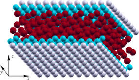
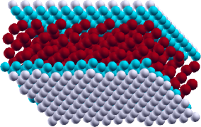
(a) (b) (c)

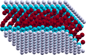
Figure 1: (Color online) Three typical stick configurations of the $N_{l}=3$ system during stick-slip motion for misfit angles (a) $\phi=0^{\circ}$, (b) $17.7^{\circ}$, and (c) $28.7^{\circ}$. Lubricant atoms are dark/red, deformable substrate atoms are clearer/blue, and fixed substrate atoms are white. Driving speed is $v=0.03$, load $f_{l}=0.1$.

As we address rather general properties of lubricated friction, we explore a relatively simple model in simulation. This allows us to span a wider range of sliding velocities and longer simulation times as well as to analyze the atomic trajectories in greater detail than by simulating fully realistic force fields appropriate to a specific system. The MD model was introduced and described in previous work BN2006 ; BP2001 ; therefore, we only discuss here its main features briefly. We study a film composed by few atomic layers and confined between two substrates, “bottom” and “top”. As illustrated in Fig. 1, each substrate consists of two layers. The external one is rigid, while the dynamics of the atoms belonging to the inner layer, the one directly in contact with the lubricant, is fully included in the model. The rigid part of the bottom substrate is held fixed, while the top substrate is mobile in the three space directions $x,y,z$.

All atoms interact with pairwise Lennard-Jones potentials

$$V(r)=V_{\alpha\alpha^{\prime}}\left[\left({r_{\alpha\alpha^{\prime}}}/{r}\right)^{12}-2\left({r_{\alpha\alpha^{\prime}}}/{r}\right)^{6}\right],$$ (1)

where $\alpha,\alpha^{\prime}=s$ or $l$ for the substrate or lubricant atoms respectively, so that the interaction parameters $V_{\alpha\alpha^{\prime}}$ and $r_{\alpha\alpha^{\prime}}$ depend on the type of atoms. Between two substrate atoms we use $V_{ss}=3$ and an equilibrium distance $r_{ss}=3$. The interaction between the substrate and the lubricant is much weaker, $V_{sl}=1/3$. For the “soft” lubricant itself, we consider $V_{ll}=1/9$ and an equilibrium spacing $r_{ll}=4.14$, which is poorly commensurate with $r_{ss}$. The equilibrium distance between the substrate and the lubricant is $r_{sl}=\frac{1}{2}(r_{ss}+r_{ll})$. For the long-range tail of all potentials we adopt a standard truncation to $r\leq r^{*}=1.49\,r_{ll}$. The atomic masses are $m_{l}=m_{s}=1$. The two substrates are pressed together by a loading force $f_{l}$ per substrate atom (typically we used the value $f_{l}=0.1$). All parameters are given in dimensionless units defined in Ref. BP2001 , for example the model units for force is $V_{ss}/r_{ss}$. The chosen parameters correspond roughly to a typical system where energy is measured in electronvolts and distances in ångströms, so that forces are in the nanonewton range.

The main difference between our technique and other simulations of confined systems lies in the dissipative coupling with the heat bath, representing the bulk of the substrates. We use Langevin dynamics with a position- and velocity-dependent damping coefficient $\eta(d_{i},v_{i})$, which is designed to mimic realistic dissipation, as discussed in Refs. BN2006 ; BP2001 . In a driven system the energy pumped into the system must be removed from it. In reality energy losses occurs through the excitation of degrees of freedom not included in the calculation, namely energy transfer into the bulk of the substrates. To model this fact, damping should occur primarily when a moving atom comes at a small distance $d_{i}$ from either substrate. Moreover, the efficiency of the energy transfer depends on the velocity $v_{i}$ of the atom because $v_{i}$ affects the frequencies of the motions that it excites within the substrates. The damping is written as $\eta(d,v)=\eta_{1}(d)\,\eta_{2}(v)$ with $\eta_{1}(d)=1-\tanh[(d-d^{*})/d^{*}]$, where $d^{*}$ is a characteristic distance of the order of one lattice spacing. The expression of $\eta_{2}(v)$ is deduced from the results known for the damping of vibrations of an atom adsorbed on a crystal surface (see Ref. BF2002 and references therein).

In simulations we explore the “spring” algorithm, where a spring is attached to the rigid top layer, and the spring end is driven at a constant velocity. We apply periodic boundary conditions (PBC) in the $x$ and $y$ directions. The geometric construction of the rotated substrate is explained in the Appendix A. In simulation, it is simpler to rotate the bottom substrate only. The initial configuration of the lubricant is prepared as a set of $N_{l}$ ($N_{l}=1$, 2, 3, and 5) closely packed atomic layers. Most simulations include $80$ atoms in each lubricant layer, although we increased the system size by up to 16 times to check for size effects. The system is then annealed, i.e., the temperature is raised adiabatically to $T\sim 0.6$, which exceeds the melting temperature $T_{m}$ ($T_{m}\simeq 0.1$ for our lubricant BP2003 ) and then decreased back to the desired value. After preparation of the annealed configuration, we perform a standard protocol of runs: starting from the high-speed $v=1$ LS regime, corresponding to a sliding speed comparable to the sound velocity of the lubricant in its solid state, we reduce the driving velocity $v$ in steps down to the value $v=0.01$ (which produces stick-slip motion for most employed simulation parameters), and then increase $v$, up to $v=3$. Typical MD snapshots are shown in Fig. 1.

To estimate $f_{s}$ in the stick-slip regime we select the $v=0.03$ runs and take an average of the peak spring force immediately prior to slip. A lower sliding speed would lead to slightly larger friction, due to longer aging of pinning contacts, but would require longer simulation times to record the same number of stick-slip events. The moderate speed $v=0.03$ realizes a fair compromise, which in practical simulation times produces a $\sim 10\%$ underestimate of $f_{s}$ with respect to its value at adiabatically slow sliding. To find the kinetic friction force $f_{k}$ in the smooth sliding regime, we average the spring force over the whole run.

III Simulation results

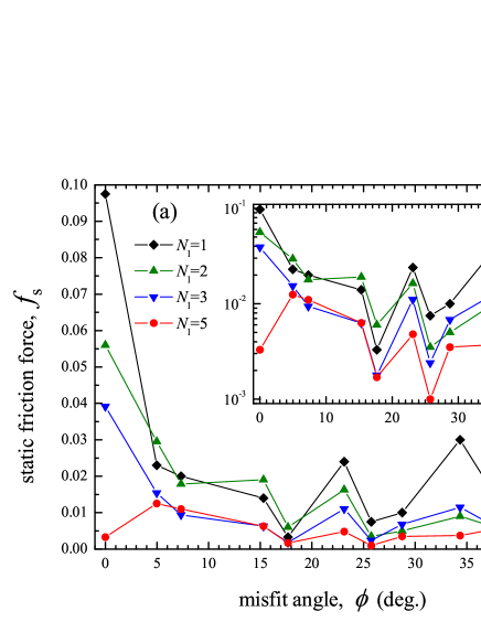
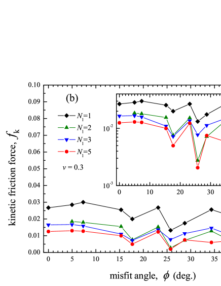
Figure 2: (Color online) Static (panel a, stick slip at $v=0.03$) and kinetic (panel b, smooth sliding with $v=0.3$) friction forces for several values of the misfit angle $\phi$ for $T=0$ and different thicknesses of the lubricant film: $N_{l}=1$ (diamonds), 2 (green up triangles), 3 (blue down triangles), and 5 (red circles). Insets display the same dependences in logarithmic scale. All forces here and in the following figures are reported in the natural model units, i.e. in units of $V_{ss}/r_{ss}$.

The simulation results are summarized in Fig. 2. Qualitatively, the results agree with those of He and Robbins HR2001s ; HR2001k , with stick-slip motion at low driving velocities and smooth sliding for $v\gtrsim 0.1$. At zero substrate temperature, the static friction can vary with the misfit angle $\phi$ by two orders of magnitude, and the kinetic friction for smooth sliding at low velocity (e.g. as shown for $v=0.3$ in Fig. 2b) by more than one order of magnitude. For the thin lubricant films, $N_{l}\leq 3$, the static friction peaks for perfectly aligned substrates, $\phi=0$. This does not occur any more for thicker films. The friction achieves sharp minima at the angles $\phi=17.7^{\circ}$, $25.7^{\circ}$ and $40.5^{\circ}$ as will be discussed below. At large driving velocities, $v\geq 1$ (which is in fact huge, comparable to the solid-lubricant sound velocity) the lubricant film is completely molten, and friction becomes almost independent of $\phi$.

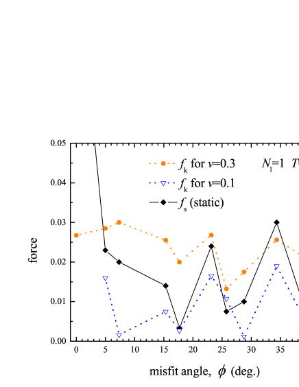
Figure 3: (Color online) Friction force as a function of the misfit angle $\phi$ for the one-layer lubricant film at $T=0$. Diamonds correspond to static friction, triangles to kinetic friction at $v=0.1$, and circles to kinetic friction at $v=0.3$.

The variation of friction with $\phi$ is the most pronounced for the one-layer lubricant film. The simulation results for this thinnest film are presented in Fig. 3. The static and low-speed ($v\leq 0.3$) kinetic friction force displays sharp minima for the angles $\phi=17.7^{\circ}$, $25.7^{\circ}$ and $40.5^{\circ}$. For these “special” angles, the lubricant film remains ordered and slides together either with the top or the bottom substrate both during slips and in smooth sliding (we call this regime as the “solid sliding”, or SS). Of course the motion is not rigid but corresponds to a “solitonic” sliding mechanism BraunBook ; Vanossi06 ; Vanossi07PRL . For the other angles studied, at stick configurations the film orders locally, with a structure adjusted partly to the bottom and partly to the top substrates, while during slips, as well as at smooth sliding, the film is 2D-melted (LS regime).

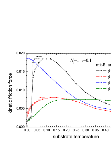
Figure 4: (Color online) Kinetic friction force as a function of temperature (in natural units of $V_{ss}/(3k_{\rm B})$, where $k_{\rm B}$ is the Boltzmann constant) computed at $v=0.1$ for the misfit angles $\phi=17.7^{\circ}$ and $\phi=40.5^{\circ}$ (solitonic), $\phi=34.3^{\circ}$ (high friction), and $\phi=7.3^{\circ}$ (fragile solitonic) for the $N_{l}=1$ system.

The dependence of the kinetic friction force on temperature is shown in Fig. 4. For all “non-special” angles, when the static friction is relatively high, the kinetic friction decreases with temperature (e.g., see the dependence for $\phi=34.3^{\circ}$ in Fig. 4), reflecting the standard thermolubric effect P0 ; BN2006 ; Gnecco00 ; Sang01 ; Riedo03 ; Gnecco03 ; Sills03 ; Jinesh08 ; Krylov08 due to temperature-assisted barrier overcoming. However, for all special angles producing the SS regime, the behavior is different: thermal fluctuations perturb a rather delicate solitonic motion, leading to an initial increase of friction with $T$. Such a behavior occurs also for thicker films. For the misfit angle $\phi\simeq 7.3^{\circ}$ we observe that at $v=0.1$ the one-layer film reaches an exceptional sliding state characterized by very low friction due to SS; this type of superlubricity is not typical, and it is quickly destroyed with the increase of either temperature (Fig. 4) or velocity (Fig. 3). Note also that the superlubric SS regime is recovered significantly after it is abandoned as temperature is lowered (dotted line, open symbols), thus opening a nontrivial hysteretic loop in the thermal cycle.

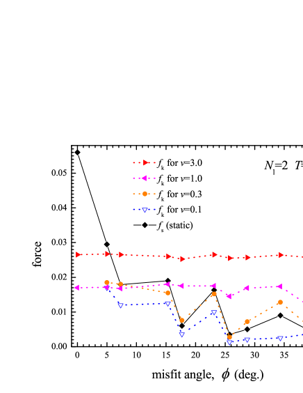
Figure 5: (Color online) Friction forces versus the misfit angle $\phi$ for the $N_{l}=2$ system. Diamonds and solid curve describe the static friction, dotted curves show the kinetic friction force at different driving speeds, up to values comparable to the lubricant sound velocity.

Consider now a thicker lubricant film with $N_{l}=2$ (see Fig. 5). For $v\geq 1$ we observe the LS regime, where the lubricant is 3D molten (except the “special” angles $\phi=25.7^{\circ}$ and $40.5^{\circ}$ at $v=1$, where we have LoLS between the two attached lubricant layers). At lower velocities, $v\leq 0.3$, the behavior is as follows. For $\phi=0$ at stick, the two ordered lubricant layers are ordered and attached to the corresponding substrates, but are 3D melted at slips. For all other angles, the LoLS regime operates during slips: for $\phi<25^{\circ}$ the attached layers are 2D molten, while for $\phi>28^{\circ}$ the attached layers remain ordered. Finally, for the angles $\phi=17.7^{\circ}$, $25.7^{\circ}$ and $40.5^{\circ}$ the friction forces exhibit deep minima produced by the SS solitonic mechanism.

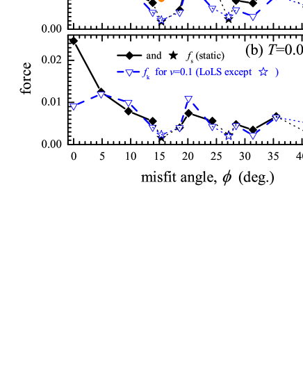
Figure 6: (Color online) Friction forces as functions of the misfit angle $\phi$ for the three-layer system. Diamonds and solid line represents static friction; stars and dotted lines mark the regime of solitonic “solid sliding” with very low friction (“superlubricity”). Dashed lines show the kinetic friction force at different driving velocities: $v=0.1$ (blue down triangles), 0.3 (orange circles), 1 (cyan left triangles) and 3 (red right triangles). Panel (a) is for $T=0$, and (b) is for the “room” temperature $T=0.025$.

We come now to describe the results for the $N_{l}=3$ system as a prototypical lubricant of mesoscale thickness. The static friction, as well as the kinetic friction in the LoLS regime, can change by more than one order in magnitude when the misfit angle varies, as illustrated in Fig. 6. $\phi=0$ produces the highest friction like for thinner lubricants. The smooth sliding, as well as slips during stick-slip, correspond to either the LoLS or the LS regime. For all other angles $\phi\neq 0$, sliding always corresponds to the LoLS regime at low driving velocities $v\leq 0.3$. Contrary to the $\phi=0$ case, now sliding is typically asymmetric and takes place at one interface only, between the middle layer and one of the attached layers, so that the middle lubricant layer sticks with either the top or the bottom substrate. The middle layer may remain ordered during sliding or, for some values of $\phi$, it is 2D-melted; in the latter case, the friction force is higher. For the special misfit angles $\phi=17.7^{\circ}$, $25.7^{\circ}$ and $40.5^{\circ}$ identified by stars in Fig. 6, we again observe the “superlubricity” characterized by the very low friction. In these cases, the lubricant film remains solid and ordered during sliding, and moves as a whole with the top or bottom substrate, in a SS sliding. However, the lubricant is not rigid during motion, thus enhancing the “solitonic” mechanism.

The results described above, remain qualitatively the same at nonzero temperatures $T<T_{m}$. For example, Fig. 6b shows the dependence of friction force on $\phi$ for the “room” temperature $T=0.025$. Both the static and kinetic (for the LoLS regime) friction forces decrease when $T$ increases. However, for the SS regime, the behavior is different – fluctuations due to temperature perturb the solitonic motion, leading to an increase of friction.

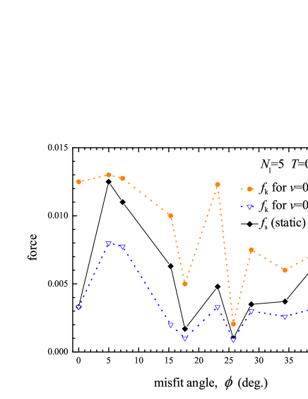
Figure 7: (Color online) Friction forces versus the misfit angle $\phi$ for the $N_{l}=5$ system. Diamonds and solid curve describe the static friction, dotted curves show the kinetic friction force at driving velocities $v=0.1$ (triangles) and 0.3 (circles).

The thicker lubricant film, $N_{l}=5$, behaves similarly to $N_{l}=3$, as illustrated in Fig. 7. The main difference is the lack of a maximum in $f_{s}(\phi)$ at $\phi=0$. Again, for the misfit angles $\phi=17.7^{\circ}$ and $25.7^{\circ}$ we observe “superlubric” sliding. For smooth sliding with $v\leq 0.3$ as well for slips during stick-slip motion, we observe either the LoLS regime, where the three central layers are 2D melted and sliding occurs between the middle layers (e.g., between layers 1-2 or 2-3), or the LS regime, where all three middle layers are 3D-molten. The LoLS regime marks the dips in $f_{k}$, while LS generates larger $f_{k}$, as occurs in the angular intervals $0^{\circ}\leq\phi\leq 10^{\circ}$ and $20^{\circ}\leq\phi\leq 25^{\circ}$. For larger velocities, $v\geq 1$, all five lubricant layers are melted and the LS regime operates in full.

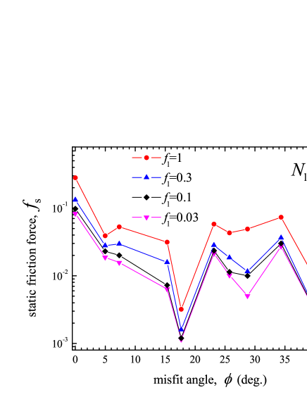
Figure 8: (Color online) Friction force versus the misfit angle $\phi$ for the $N_{l}=1$ system, driven at $v=0.01$, for different values of the applied load $f_{l}$.

Figure 8 reports the friction force for 4 values of the applied load. These calculations demonstrate that the dependency of friction on the substrate rotation is very similar for different loads, with a general increase of friction with load. We obtain very similar results for $N_{l}=2$ and 3. However, for thicker films, $N_{l}=5$, the situation changes dramatically at high load ($f_{l}=1$): the film rearranges into a closely packed four-layer configuration which remains solid under sliding. As a consequence, the peak structure of friction as a function of $\phi$ changes as well, because the lubricant structure acquires more atoms per layer and changes symmetry.

Figure 9: (Color online) The probability distribution of static thresholds for $N_{l}=1$, 2, 3 and 5 (insets) and the averaged distribution $P_{c}(f_{s})$. These distributions are obtained in the assumption that all misfit angles $\phi$ are equally likely. The calculated function $P_{c}(f_{s})$ may be approximately fitted by the distribution $P_{c}(f_{s})=\bar{f}^{-2}f_{s}\exp(-f_{s}/\bar{f})$ with $\bar{f}=0.005$.

Because the static friction varies over such a large interval, its specific value for a given misfit angle $\phi$ has little importance. Indeed one could hardly control the misfit angle in a real system, except in especially favorable situations DVPFHZ2004 . Moreover, a system where the sliding surfaces have an ideal crystalline structure oriented with a controllable $\phi$ is exceptional. Real surfaces usually have areas (domains) with different orientation. For polycrystalline substrates, it is reasonable to assume that all angles are presented with equal likeliness. It may then be more interesting to examine the probability distribution of $f_{s}$ values, regardless of $\phi$. The insets of Fig. 9 report the histograms of forces as resulting from our simulations of different thicknesses.

Besides, if we also assume that the lubricant film is not uniform but has different thickness at different places (it is certainly so if the surfaces have some roughness), then we can average over different thicknesses; the resulting distribution $P_{c}(f_{s})$ is shown Fig. 9. It is precisely this distribution which represents the main output of our MD simulations, as it then allows us to predict tribological behavior of the system with the help of a master-equation approach BP2008 . The calculation summarized in Fig. 9 are carried out at $f_{l}=0.1$. The effect of a load increase would be mainly to scale the $P_{c}(f_{s})$ distribution, so that it would peak at larger friction. The resulting distribution displays several spikes which are likely due to the fixed size of the simulated contact. We will investigate the role of contact size on the $P_{c}(f_{s})$ distribution using a simplified model, in a separate publication friction_rigid .

IV Discussion and Conclusions

The main results of the present work can be summarized as follows: (i) The relative rotation of sliding contacts in a lubricated context promotes LoLS more frequently then the standard LS. (ii) For a few special angles LoLS leads to superlubric sliding completely analogous of the unlubricated sliding of misaligned perfect crystalline substrates. This superlubric regime is however delicate and can be suppressed by small relative rotations of the substrates, by temperature, or by velocity-induced local heating. (iii) In a regime of boundary lubrication, friction forces do vary quite significantly with the relative substrate relative orientation $\phi$, even when the lubricant film becomes several atomic layers thick. (iv) To describe macroscopic friction in a context of multiasperity contact, where relative orientation is not really under control, the most important information to be extracted from MD simulations is a probability distribution $P_{c}(f_{s})$ rather than specific values of the static friction force $f_{s}$.

The present calculation is consistent with a rapidly (approximately exponentially) decaying distribution $P_{c}(f_{s})$, up to a cutoff force related to the average contact size. When temperature can promote rotations, beside the standard reduction of friction at low speed due to thermal crossing of barriers, thermal fluctuations could affect the barrier distribution itself by suppressing small barriers in favor of higher ones FDFKU2008 .

Appendix A The construction of the rotated substrate

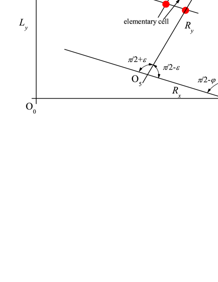
Figure 10: (Color online) Construction of the rotated lattice.

In this Appendix we report the construction of the substrate rotated by a given misfit angle $\phi$. The main problem here is to obtain numerous misfit angles $\phi$ which satisfy PBC in $x$ and $y$ directions simultaneously, while maintaining a constant simulation size, and rectangular PBC (for the square shape of the simulation cell the construction is much simpler, e.g., see Ref. GT1997 ). The idea of the construction is demonstrated in Fig. 10. The substrate is arranged according to a square lattice with lattice constant $a_{s}$, and the simulation cell area is $L_{x}\times L_{y}=M_{x}a_{s}\times M_{y}a_{s}$. The rotated bottom lattice is constructed as a set of parallelograms, so that the elementary cell of the new lattice has size $a_{x}\times a_{y}$ with a base angle $\pi/2+\varepsilon$. In the perfect case we would have $a_{x}=a_{y}=a_{s}$ and $\varepsilon=0$. However, to satisfy the PBC, the rotated lattice has to be distorted from the ideal square shape, and the idea is to reduce this distortion to a minimum.

The rotated lattice is defined by two integers $n_{1}$ and $n_{2}$ (see Fig. 10) which determine the rotation angle $\varphi$. For example, the choice $n_{1}=M_{x}$ and $n_{2}=0$ or $n_{1}=0$ and $n_{2}=M_{y}$ gives the original square lattice, while the sets $n_{1}=M_{x}$ and $n_{2}=1$ or $n_{1}=1$ and $n_{2}=M_{y}$ lead to the minimally allowed misfit angle for the given size of the simulation cell. Let us draw two lines (see Fig. 10), the first line starts at the point O${}_{2}=(0,L_{y})$ and has the length $n_{1}a_{x}$, while the second line starts at the point O${}_{3}=(L_{x},L_{y})$ and has the length $n_{2}a_{y}$. These lines intersect at point O₄ forming an angle $\pi/2+\varepsilon$. The rotated substrate atoms are placed along these lines, and then periodic shifts by multiples of $a_{x}$ and $a_{y}$ in the directions defined by these two lines will generate the rotated oblique lattice.

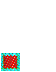
(a) (b)

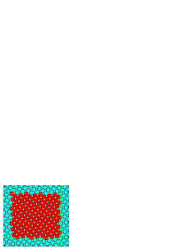
Figure 11: (Color online) Two typical examples of the rotated substrate lattice, with $M_{x}=12$ and $M_{y}=11$: (a) for $\phi=28.75^{\circ}$ ($n_{1}=10$, $n_{2}=6$, $\varepsilon=0.58^{\circ}$, $a_{x}=3.15$, $a_{y}=2.86$, $\Delta N_{\rm sub}=-2$, $\delta_{1}=0.0294$), and (b) for $\phi=34.35^{\circ}$ ($n_{1}=10$, $n_{2}=7$, $\varepsilon=-2.3^{\circ}$, $a_{x}=3.01$, $a_{y}=2.99$, $\Delta N_{\rm sub}=0$, $\delta_{1}=10^{-9}$). The atoms are shown by circles: those within the simulation cell are red/dark, while their periodic “images” are cyan/clear.

The oblique lattice constants $a_{x}$ and $a_{y}$ are determined by two constrains. First, we must preserve the area of the elementary cell:

$$a_{x}a_{y}\cos\varepsilon=a_{s}^{2}\,.$$ (2)

Second, from the triangle O₂O₃O₄ we have

$$L_{x}^{2}=\left(n_{1}a_{x}\right)^{2}+\left(n_{2}a_{y}\right)^{2}+2n_{1}\,n_{2}\,a_{s}^{2}\tan\varepsilon\,.$$ (3)

From Eqs. (2) and (3) we obtain

$$\left(a_{x}^{2}\right)_{1,2}=\left(A\cos^{2}\varepsilon\pm D\right)/\left(2n_{1}^{2}\cos^{2}\varepsilon\right),$$ (4)

where $D=\left(A^{2}\cos^{2}\varepsilon-4n_{1}^{2}n_{2}^{2}a_{s}^{4}\right)^{1/2}\cos\varepsilon$ and $A=L_{x}^{2}-2n_{1}n_{2}a_{s}^{2}\tan\varepsilon$. The signs $\pm$ in Eq. (4) yield two possible solutions which we call as “left” and “right”; typically we use the “right” variant when $n_{1}>M_{x}/2$ and the “left” one for $n_{1}<M_{x}/2$. Finally, the actual misfit angle $\phi$ is given by $\phi=\varphi+\varepsilon/2$, where

$$\sin\varphi=n_{2}a_{y}\cos\varepsilon/L_{x}.$$ (5)

The construction described above guarantees the perfect PBC in the $x$ direction, but not in the $y$ one. Therefore, a next step in construction is to characterize this distortion. Considering the triangle O₁O₃O₅ in Fig. 10 (the line O₁O₅ is parallel to O₂O₄), the lengths of its short sides are $R_{x}=R_{B}\sin(\varphi+\varepsilon)$ and $R_{y}=R_{B}\cos\varphi$, where $R_{B}=L_{y}/\cos\varepsilon$. The distortion of PBC is determined by two parameters $\delta_{x}=\left[R_{x}/a_{x}-{\rm int}(R_{x}/a_{x})\right]^{2}$ and $\delta_{y}=\left[R_{y}/a_{y}-{\rm int}(R_{y}/a_{y})\right]^{2}$. In the ideal case, it should be $\delta_{x}=\delta_{y}=0$.

A “quality” of the rotated lattice can be characterized by two parameters: the first parameter

$$\delta_{1}=\delta_{x}^{2}+\delta_{y}^{2}$$ (6)

describes the distortion of periodic boundary conditions, while the second parameter

$$\delta_{2}=(a_{x}/a_{y}-1)^{2}$$ (7)

indicates how close $a_{x}$ and $a_{y}$ are to the original square-lattice constant $a_{s}$. Perfect rotations are realized for $\delta_{1}=0$ and $\delta_{2}=0$ simultaneously at $\varepsilon=0$. Thus, for given integers $n_{1}$ and $n_{2}$, we plot $\delta_{1}$ and $\delta_{2}$ as functions of $\varepsilon$, to choose an appropriate minimum of $\delta_{1}(\varepsilon)$ close to the point $\varepsilon=0$, and to check that $\delta_{2}$ is not too large at that point.

Note that in the non-ideal case, some atoms within the $L_{x}\times L_{y}$ simulation cell may be missing or, for other sets of parameters, some atoms may overlap with their “image” atoms generated by PBC. To overcome this problem, we shifted slightly the bottom boundary of the selected area. As a result, in the rotated lattice the number of substrate atoms may differ from the original one by a value $\Delta N_{\rm sub}$.

Finally, because different sets of parameters may provide approximately the same misfit angle, we can choose the best set, the one which minimizes $\delta_{1,2}$ and $\varepsilon$. Two typical examples of the construction described above are shown in Fig. 11.

References

- (1) B.N.J. Persson, “Sliding Friction: Physical Principles and Applications” (Springer-Verlag, Berlin, 1998).
- (2) O.M. Braun and A.G. Naumovets, Surf. Sci. Reports 60, 79 (2006).
- (3) P.A. Thompson and M.O. Robbins, Phys. Rev. A41, 6830 (1990).
- (4) P.A. Thompson and M.O. Robbins, Science 250, 792 (1990); M.O. Robbins and P.A. Thompson, Science 253, 916 (1991).
- (5) M. Hirano and K. Shinjo, Phys. Rev. B41, 11837 (1990).
- (6) M.H. Müser and M.O. Robbins, Phys. Rev. B61, 2335 (2000).
- (7) G. He, M.H. Müser, and M.O. Robbins, Science 284, 1650 (1999).
- (8) M.H. Müser, L. Wenning, and M.O. Robbins, Phys. Rev. Lett. 86, 1295 (2001).
- (9) F. Lancon, Europhys. Lett. 57, 74 (2002).
- (10) M. Hirano and K. Shinjo, Wear 168, 121 (1993).
- (11) M.O. Robbins and E.D. Smith, Langmuir 12, 4543 (1996).
- (12) G.S. Verhoeven, M. Dienwiebel, and J.W.M. Frenken, Phys. Rev. B70, 165418 (2004).
- (13) F. Bonelli, N. Manini, E. Cadelano, and L. Colombo, Eur. Phys. J. B 70, 449 (2009).
- (14) A.S. de Wijn, C. Fusco, and A. Fasolino, Phys. Rev. E81, 046105 (2010).
- (15) T. Gyalog and H. Thomas, Europhys. Lett. 37, 195 (1997).
- (16) Y. Qi, Y.-T. Cheng, T. Cagin, and W.A. Goddard III, Phys. Rev. B66, 085420 (2002).
- (17) M. Hirano, K. Shinjo, R. Kaneko, and Y. Murata, Phys. Rev. Lett. 78, 1448 (1997).
- (18) M. Dienwiebel, G.S. Verhoeven, N. Pradeep, J.W.M. Frenken, J.A. Heimberg, and H.W. Zandbergen, Phys. Rev. Lett. 92, 126101 (2004).
- (19) G. He and M.O. Robbins, Phys. Rev. B64, 035413 (2001).
- (20) G. He and M.O. Robbins, Tribology Letters 10, 7 (2001).
- (21) O.M. Braun and M. Peyrard, Phys. Rev. E63, 046110 (2001).
- (22) O.M. Braun and R. Ferrando, Phys. Rev. E65, 061107 (2002).
- (23) O.M. Braun and M. Peyrard, Phys. Rev. E68, 011506 (2003).
- (24) O.M. Braun and Yu.S. Kivshar, “The Frenkel-Kontorova Model: Concepts, Methods, and Applications” (Springer-Verlag, Berlin, 2004).
- (25) A. Vanossi, N. Manini, G. Divitini, G.E. Santoro, and E. Tosatti, Phys. Rev. Lett. 97, 056101 (2006).
- (26) A. Vanossi, N. Manini, F. Caruso, G.E. Santoro, and E. Tosatti, Phys. Rev. Lett. 99, 206101 (2007).
- (27) E. Gnecco, R. Bennewitz, T. Gyalog, Ch. Loppacher, M. Bammerlin, E. Meyer, and H.-J. Güntherodt, Phys. Rev. Lett. 84, 1172 (2000).
- (28) Y. Sang, M. Dubé, and M. Grant, Phys. Rev. Lett. 87, 174301 (2001).
- (29) E. Gnecco, R. Bennewitz, A. Socoliuc, and E. Meyer, Wear 254, 859 (2003).
- (30) S. Sills and R. M. Overney, Phys. Rev. Lett. 91, 095501 (2003).
- (31) E. Riedo, E. Gnecco, R. Bennewitz, E. Meyer, and H. Brune, Phys. Rev. Lett. 91, 084502 (2003).
- (32) K.B. Jinesh, S.Yu. Krylov, H. Valk, M. Dienwiebel, and J.W.M. Frenken, Phys. Rev. B78, 155440 (2008).
- (33) S. Yu. Krylov, and J. W. M. Frenken, J. Phys.: Condens. Matter 20, 354003 (2008).
- (34) O.M. Braun and M. Peyrard, Phys. Rev. Lett. 100, 125501 (2008).
- (35) N. Manini and O.M. Braun, following paper.
- (36) A.E. Filippov, M. Dienwiebel, J.W.M. Frenken, J. Klafter, and M. Urbakh, Phys. Rev. Lett. 100, 046102 (2008).