Comparison of Halo Detection from Noisy Weak Lensing Convergence Maps with Gaussian Smoothing and MRLens Treatment

Abstract

Taking into account the noise from intrinsic ellipticities of source galaxies, we study the efficiency and completeness of halo detections from weak lensing convergence maps. Particularly, with numerical simulations, we compare the Gaussian filter with the so called MRLens treatment based on the modification of the Maximum Entropy Method. For a pure noise field without lensing signals, a Gaussian smoothing results a residual noise field that is approximately Gaussian in statistics if a large enough number of galaxies are included in the smoothing window. On the other hand, the noise field after the MRLens treatment is significantly non-Gaussian, resulting complications in characterizing the noise effects. Considering weak-lensing cluster detections, although the MRLens treatment effectively deletes false peaks arising from noise, it removes the real peaks heavily due to its inability to distinguish real signals with relatively low amplitudes from noise in its restoration process. The higher the noise level is, the larger the removal effects are for the real peaks. For a survey with a source density $n_{g}\sim 30\hbox{ arcmin}^{-2}$, the number of peaks found in an area of $3\times 3\hbox{ deg}^{2}$ after MRLens filtering is only $\sim 50$ for the detection threshold $\kappa=0.02$, while the number of halos with $M>5\times 10^{13}\hbox{ M}_{\odot}$ and with redshift $z\leq 2$ in the same area is expected to be $\sim 530$. For the Gaussian smoothing treatment, the number of detections is $\sim 260$, much larger than that of the MRLens. The Gaussianity of the noise statistics in the Gaussian smoothing case adds further advantages for this method to circumvent the problem of the relatively low efficiency in weak-lensing cluster detections. Therefore, in studies aiming to construct large cluster samples from weak-lensing surveys, the Gaussian smoothing method performs significantly better than the MRLens.

1 Introduction

The weak gravitational lensing effect provides a unique tool in measuring the matter distribution in the universe (e.g., Bartelmann & Schneider 2001; Hoekstra et al. 2006; Massey et al. 2007). Its additional dependence on the distances to the source, to the lens and between the source and lens makes it an excellent probe in cosmological studies of dark energy (e.g., Albrecht et al. 2006; Benjamin et al. 2007; Kilbinger et al. 2009; Li et al. 2009). On the other hand, however, different observational and physical effects can affect the weak lensing analyses significantly. Being extracted from shape distortion of background galaxies, the weak lensing effect on individual source galaxies is severely contaminated by their intrinsic ellipticities. Therefore statistical analyses on a large number of galaxies are necessary in weak lensing studies. Even so, intrinsic shape alignments of galaxies, including intrinsic-intrinsic and shear-intrinsic correlations, can be an important source of error in cosmic shear correlation analyses. For cluster detections from weak lensing convergence maps reconstructed from shear measurements (e.g., Kaiser & Squires 1993; Bartelmann 1995; Kaiser 1995; Schneider & Seitz 1995; Squires & Kaiser 1996; Bridle et al.1998; Marshall et al. 2002), even randomly orientated intrinsic ellipticities can result false peaks by their chance alignments, which can reduce the efficiency of cluster detections significantly (e.g., Schneider 1996; van Waerbeke 2000; White et al. 2002; Hamana et al. 2004; Fan 2007). Thus further treatments for a convergence map are normally required to suppress the noise effects.

The noise from intrinsic ellipticities of source galaxies is essentially shot noise, and thus by averaging over a relatively large number of source galaxies in weak lensing analyses, the residual noise can be effectively reduced. This leads to the normal smoothing treatment. It is clear that the residual noise depends on the form of the window function and the smoothing scale. For a Gaussian smoothing with a window function of the form $W(\theta)\propto\exp(-\theta^{2}/\theta_{G}^{2})$, the residual noise can be estimated by $\sigma^{2}_{0}\approx{(\sigma^{2}_{\epsilon}/2)}{[1/(2\pi\theta_{G}^{2}n_{g})]}$, where $\sigma_{\epsilon}$ is the rms of the intrinsic ellipticity of individual source galaxies, $\theta_{G}$ is the smoothing scale, and $n_{g}$ is the surface number density of source galaxies. For $\sigma_{\epsilon}=0.3$, $n_{g}=30\hbox{ arcmin}^{-2}$ and $\theta_{G}=1\hbox{ arcmin}$, we have $\sigma_{0}\approx 0.015$.

Recently, Starck et al. (2006) proposed the MRLens filtering technique, which is based on the Bayesian analyses with a multi-scale entropy prior applied. The False Detection Rate (FDR) method is used to select significant/non-significant wavelet coefficients (e.g., Starck et al. 2006; Pires et al. 2009). The MRLens method suppresses noise adaptively according to the strength of the noise itself. A more detailed description of the method is given in §4.

In this paper, with numerical simulations, we compare Gaussian smoothing with MRLens treatment, paying particular attention to the completeness and the efficiency of weak lensing halo detections from convergence maps. The rest of the paper is organized as follows. In §2, we describe briefly the weak-lensing convergence reconstruction and the Gaussian smoothing. In §3, we present the important aspects of the MRLens treatment. Results are shown in §4. Section 5 contains summaries and discussions.

2 Weak lensing convergence reconstruction

In the weak lensing regime, the convergence $\kappa(\vec{\theta})$ is essentially related to the weighted projection of density fluctuations $\delta$ along the unperturbed light path. Specifically, we have

$$\kappa(\vec{\theta})={3H_{0}^{2}\Omega_{0}\over 2}\int_{0}^{w_{H}}dw\bar{W}(w)f_{K}(w){\delta[f_{K}(w)\vec{\theta},w]\over a(w)}$$ (1)

where $H_{0}$ is the present Hubble constant, $\Omega_{0}$ is the present matter density of the universe in unit of the critical density, ${w}$ is the radial coordinate, $a(w)$ is the scale factor of the universe, and, with $K$ being the spatial curvature of the universe,

$$f_{K}(w) =|K|^{-1/2}\sin(|K|^{1/2}w)\quad\quad\ \ \ (K>0)$$ (2)

$$=w\qquad\qquad\qquad\qquad\qquad\quad(K=0)$$

$$=|K|^{-1/2}\sinh(|K|^{1/2}w)\qquad(K<0)\ .$$

The factor $\bar{W}(w)$ is the weighting function that is related to the source galaxy distribution $G(w)$ by

$$\bar{W}(w)=\int_{w}^{w_{H}}dw^{\prime}G(w^{\prime}){f_{K}(w^{\prime}-w)\over f_{K}(w^{\prime})}\ .$$ (3)

The lensing potential $\phi$ is related to $\kappa$ by

$$\kappa={\nabla^{2}\phi\over 2}\ ,$$ (4)

and the shears $\gamma_{1}$ and $\gamma_{2}$ are

$$\gamma_{1}={\partial_{11}\phi-\partial_{22}\phi\over 2}\ ,\quad\gamma_{2}=\partial_{12}\phi.$$ (5)

Since both $\kappa$ and $\gamma_{i}$ are determined by the lensing potential, they are mutually dependent of each other. In the Fourier space, we have (Kaiser & Squires 1993)

$$\kappa(\vec{k})=c_{1}(k)\gamma_{1}(\vec{k})+c_{2}(k)\gamma_{2}(\vec{k}),$$ (6)

where $[c_{1},c_{2}]=[\cos(2\phi),\sin(2\phi)]$ with $\vec{k}=k(\cos\phi,\sin\phi)$.

Observationally, the shear $\gamma$ can be extracted from the shape measurement of source galaxy images. Under the condition $\kappa<<1$, we have

$$\vec{e}^{\rm obs}\approx\vec{\gamma}+\vec{e}^{S}\ ,$$ (7)

where $\vec{e}^{\rm obs}$ and $\vec{e}^{S}$ are the observed ellipticity, and the intrinsic ellipticity of a source galaxy, respectively. Reconstructed from $\vec{e}^{\rm obs}$, the convergence $\kappa_{n}(\vec{k})$ then contains noise from the intrinsic part, i.e.,

$$\kappa_{n}({\vec{k}})=c_{\alpha}(k)e^{\rm obs}_{\alpha}({\vec{k}})=\kappa({\vec{k}})+c_{\alpha}(k)e^{S}_{\alpha}({\vec{k}}).$$ (8)

With the transformation back to the real 2-D space and applying a smoothing with the window function $W(\vec{\theta})$, we can obtain the smoothed quantities (e.g., van Waerbeke 2000)

$$\Sigma^{\rm obs}(\vec{\theta})=\Gamma(\vec{\theta})+\frac{1}{n_{g}}\Sigma^{N_{g}}_{i=1}W(\vec{\theta}-\vec{\theta}_{i})e^{\rm S}(\vec{\theta}_{i})$$ (9)

and

$$K_{N}(\vec{\theta})=\int d\vec{k}e^{-i\vec{k}\cdot\vec{\theta}}c_{\alpha}(k)\Sigma_{\alpha}^{\rm obs}(\vec{k}),$$ (10)

where $\Sigma^{\rm obs}$, $\Gamma$, and $K_{N}$ are the smoothed $e^{\rm obs}$, $\gamma$ and $\kappa_{n}$, respectively, and $n_{g}$ and $N_{g}$ are the surface number density and the total number of source galaxies in the field. The noise part of $K_{N}$ due to the intrinsic ellipticities is then

$$N(\vec{\theta})=\frac{1}{n_{g}}\Sigma^{N_{g}}_{i=1}\int d\vec{k}W(\vec{k})e^{-i\vec{k}\cdot(\vec{\theta}-\vec{\theta}_{i})}c_{\alpha}(k)e^{S}_{\alpha}(\vec{\theta}_{i}),$$ (11)

where $W(\vec{k})$ is the Fourier transformation of the window function with the form

$$W(\vec{k})=\frac{1}{(2\pi)^{2}}\int d\vec{\theta}e^{i\vec{k}\cdot\vec{\theta}}W(\vec{\theta}).$$ (12)

Without considering the intrinsic alignment of $e^{S}$, it is expected from the central limit theorem that the smoothed noise field $N(\vec{\theta})$ is approximately Gaussian in statistics if the effective number of galaxies included in the smoothing window is larger than about $10$ (e.g., van Waerbeke 2000). In this case, smoothing leads to correlations in $N(\vec{\theta})$, and its two-point correlation function is approximately

$$<N(\vec{\theta})N(\vec{\theta}^{\prime})>=\frac{\sigma_{\epsilon^{2}}}{2n_{g}}(2\pi)^{2}\int d\vec{k}e^{i\vec{k}\cdot(\vec{\theta}^{\prime}-\vec{\theta})}|W(\vec{k})|^{2},$$ (13)

where $\sigma_{\epsilon}$ is the intrinsic dispersion of $e^{\rm obs}$.

The approximate Gaussianity of $N(\vec{\theta})$ allows us to quantify the noise effects straightforwardly. The noise effects on cluster mass reconstruction and the noise peak statistics are analyzed in van Waerbeke (2000). Even with weak alignments of intrinsic ellipticities, $N(\vec{\theta})$ can still be approximately described by a Gaussian random field with a modified two-point correlation function including the effects of intrinsic alignments. The enhancement of the noise peak abundance due to the weakly intrinsic alignments are analyzed in Fan (2007). In Fan et al. (2010), the effects of the presence of real dark matter halos on the noise peak statistics around them as well as the effects of the noise on the peak height of real halos are investigated in detail. They further present a model to calculate the total peak abundance in a large-scale convergence map, including the peaks corresponding to real halos and the noise peaks from the chance alignment of the intrinsic ellipticities of source galaxies. Such a model makes it possible for us to use directly the peaks from convergence maps as cosmological probes without the need to differentiate real and false peaks.

Due to its simple operational procedure and the Gaussian statistics of the residual noise field, the smoothing treatment has been widely applied in weak lensing analyses. Different smoothing functions have been used in different studies. In this paper, we consider the Gaussian smoothing function $W_{G}$, which is one of the most commonly adopted window functions. Specifically, we have

$$W_{G}=\frac{1}{\pi\theta_{G}^{2}}\exp\left(-\frac{\theta^{2}}{\theta_{G}^{2}}\right)\ ,$$ (14)

where $\theta_{G}$ is the smoothing scale. Then from Eq. (13), the rms of the noise $\sigma_{0}$ after smoothing is given by

$$\sigma_{0}^{2}={\sigma_{\epsilon}^{2}\over 2}{1\over 2\pi\theta_{G}^{2}n_{g}}\ .$$ (15)

In our analyses, we choose $\sigma_{\epsilon}=0.3$, the typical value for lensing source galaxies, and $\theta_{G}=1\hbox{ arcmin}$, which is the optimal smoothing scale considering cluster-sized halos. Then for a lensing survey with $n_{g}=30\hbox{ arcmin}^{-2}$, $\sigma_{0}\approx 0.015$, which is about $20$ times lower than $\sigma_{\epsilon}$.

3 MRLens method

Starck et al. (2006) introduce a new reconstruction and filtering method, namely, Multi-scale Entropy Restoration (MRLens). It is developed from the Maximum Entropy Method. The basic idea is to use only ‘signals’ selected by the so called False Discovery Rate (FDR) (Benjamini & Hochberg 1995) to reconstruct the convergence field through a Multi-scale Entropy prior. In the following, we present specific steps of MRLens.

3.1 Wavelet decomposition

For an original convergence map $\kappa_{obs}$ with $N=n\times n$ pixels, the first step of MRLens is to decompose the image map into different components representing fine structures of different scales.

To do this, we first initialize $j=0$ and set $C_{0}(k,l)=\kappa_{obs}(k,l)$, i.e., $j=0$ corresponds to the unprocessed map with detailed structures. Then we progressively go to higher $j$ to obtain smoother maps through (Starck et al. 2001)

$$C_{j+1}(k,l)=\sum_{m}\sum_{n}h_{1D}(m)h_{1D}(n)C_{j}(k+2^{j}m,l+2^{j}n),$$ (16)

where $h_{1D}(m)={[1/16,4/16,6/16,4/16,1/16]}$ for $m=-2,-1,0,1,2$, respectively. Defining

$$w_{j+1}(k,l)=C_{j}(k,l)-C_{j+1}(k,l),$$ (17)

we finally obtain

$$\kappa_{obs}(k,l)=C_{J}(k,l)+\sum_{j=1}^{J}w_{j}(k.l),$$ (18)

where $J$ is a chosen number determined by specific considerations on how smooth we want to go. Here we set $J=7$. In our following analyses, each map is $3\times 3\hbox{ deg}^{2}$ discretized into $1024\times 1024$ pixels. Thus $2^{J}=128$ pixels corresponding to $\sim 22\hbox{ arcmin}$. Because we do not expect to see significant structures resulting purely from noise on such a large scale, $J=7$ is an appropriate choice.

It can be seen from Eq. (18) that $C_{J}(k,l)$ is the most smoothed version of the original map $\kappa_{obs}$, and the terms in the summation contain ever smaller-scale information with smaller $j$.

3.2 Multiscale Entropy

With the multi-scale wavelet decomposition, one can then construct an entropy with the obtained wavelet coefficients $w_{j}(k,l)$ at each grid $(k,l)$ with $j=1,2,...,J$. It can generally be written as

$$H(\kappa)=\sum_{k,l}h[C_{J}(k,l)]+\sum_{j=1}^{J}\sum_{k,l}h[w_{j}(k,l)].$$ (19)

For $h$, there are different definitions (e.g., Starck et al. 2006).

Here we follow Starck et al. (2001) to choose the entropy of NOISE-MSE $h_{n}$ in our considerations. At each scale $j$, the noise entropy at each grid $(k,l)$ is derived by weighting the entropy with a probability that $w_{j}(k,l)$ is contributed by noise. Specifically, we have

$$h_{n}[w_{j}(k,l)]=\int_{0}^{\mid w_{j}(k,l)\mid}P_{n}[\mid w_{j}(k,l)\mid-u]\frac{\partial h(x)}{\partial x}|_{x=u}du,$$ (20)

where $P_{n}[w_{j}(k,l)]$ is the probability that the coefficient $w_{j}(k,l)$ can be due to noise, and is given by

$$P_{n}[w_{j}(k,l)]=\mathrm{Prob}[W>\mid w_{j}(k,l)\mid].$$ (21)

Eq. (20) essentially regards the information contained in $w_{j}(k,l)$ to be built up from the summation of $dh(u)$. For each newly added $dh(u)$, depending on the difference $|w_{j}(k,l)|-u$, there is a probability that it is due to noise.

For Gaussian noise with rms $\sigma_{j}$ at scale $j$, we have

$$P_{n}[w_{j}(k,l)] = \frac{2}{\sqrt{2\pi}\sigma_{j}}\int_{\mid w_{j}(k,l)\mid}^{+\infty}\exp(-W^{2}/2\sigma^{2}_{j})dW$$ (22)

$$= \mbox{erfc}\bigg{(}\frac{\mid w_{j,k,l}\mid}{\sqrt{2}\sigma_{j}}\bigg{)}$$

and thus

$$h_{n}[w_{j}(k,l)]=\frac{1}{\sigma_{j}^{2}}\int_{0}^{\mid w_{j}(k,l)\mid}u\mbox{ erfc}\bigg{(}\frac{\mid w_{j}(k,l)\mid-u}{\sqrt{2}\sigma_{j}}\bigg{)}du.$$ (23)

3.3 Selecting significant wavelet coefficients using the False Discovery Rate (FDR)

The Multiscale Entropy method applies regularizations on wavelet coefficients to minimize noise contributions while keeping the signal information. Thus for those coefficients which are clearly signals, they should be kept unchanged. Then a new Multiscale Entropy is defined as (e.g., Starck et al. 2006)

$$\tilde{h}_{n}[w_{j}(k,l)]=\bar{M}_{j}(k,l)h_{n}[w_{j}(k,l)],$$ (24)

where

$$\bar{M}_{j}(k,l)=1-M_{j}(k,l),$$ (25)

and $M$ is the multi-resolution support defined as (Starck et al. 1995)

$$M_{j}(k,l)=\{\begin{array}[]{ll}1&\textrm{if $w_{j}(k,l)$ is significant}\\ 0&\textrm{if $w_{j}(k,l)$ is not significant}\end{array}.$$ (26)

Therefore $\tilde{h}_{n}$ means that we only need to regularize those wavelet coefficients which are ^′not significant^′, that is, they are likely due to noise.

For judging the significance of a wavelet coefficient, a commonly used criterion is a ‘$k\sigma$’ threshold. If a coefficient is above the threshold, it is defined to be ^′significant^′. This is equivalent to set a threshold for the ratio of ^′significant^′ detections over the total number of pixels being analyzed. Considering a Gaussian noise, a $2\sigma$ criterion corresponds to a probability of $0.05$ for a noise coefficient being mis-classified as ^′significant^′. If we have totally $N$ pixels to consider, the number of false discoveries is then on average $0.05N$. If the number of pixels related to real signals in the analyses is comparable to $0.05N$, the false discovery rate with respect to the number of real signals can be much higher than $0.05$. Increasing $k$ can lower the number of false detections at the expense, however, of the power of real detections. To overcome such difficulties, an alternative thresholding technique, the False Discovery Rate (FDR), has been proposed (Benjamini & Hochberg 1995; Miller et al. 2001; Hopkins et al. 2002; Starck et al. 2006).

This method can effectively control, in an adaptive manner, the fraction of false discoveries over the total number of discoveries, rather than over the total number of pixels analyzed.

Let $P_{1},\ldots,P_{N}$ denote the p-values ordered from low to high for the N pixels, where p-value is defined as

$$p_{value}=\frac{1}{\sqrt{2\pi}\sigma_{j}}\int_{w_{j}(k,l)}^{\infty}\exp[-(w-\bar{w}_{j})^{2}/2\sigma^{2}_{j}]dw,$$ (27)

with $\bar{w}_{j}$ the average of $w_{j}(k,l)$ for the scale $j$ over all the pixels. Define

$$d_{j}=\max\left\{k_{j}:\ P_{k_{j}}<\frac{k_{j}\alpha_{j}}{c_{N}N}\right\},$$ (28)

then all the $w_{j}(k,l)$ with their values larger than $d_{j}$ are classified as ^′significant^′. Here $c_{N}=1$ if all the pixels are statistically independent. The meaning of $\alpha_{j}$ is approximately the pre-defined false discovery rate at scale $j$ with respect to the total number of detections. The larger the $\alpha_{j}$ value, the larger the fraction of $w_{j}(k,l)$ defined to be ^′significant^′. In our analyses, we adopt FDR to find the values of $M$ in Eq. (26). In the MRLens program, $\alpha_{0}$ is an adjustable parameter, and $\alpha_{j}=\alpha_{0}\times 2^{j}$ (Starck et al. 2006).

3.4 Multi-scale Entropy Filtering algorithm

Given the discussions in the previous subsections, the Multi-scale Entropy restoration method reduces to find the reconstructed $\kappa_{f}$ that minimizes $I(\kappa_{f})$ defined as

$$I({\kappa_{f}})=\frac{\parallel{\kappa_{obs}-\kappa_{f}\parallel^{2}}}{2\sigma_{n}^{2}}+\beta\sum_{j=1}^{J}\sum_{k,l}\tilde{h}_{n}[({\cal W}{\kappa_{f}})_{j}(k,l)],$$ (29)

where $\sigma_{n}$ is the rms of noise in the original convergence map $\kappa_{obs}$, $J$ is the number of wavelet scales, $\cal W$ is the wavelet transform operator and $\tilde{h}_{n}[({\cal W}{\kappa_{f}})_{j}(k,l)]$ is the multi-scale entropy defined only for non-significant coefficients selected by the FDR method. The $\beta$ parameter is calculated under the restriction that the residual should have a standard deviation equal to the rms of noise. The best $\kappa_{f}$ is then obtained by iterative calculations. Full details of the minimization algorithm can be found in Starck et al. (2001).

It can be seen that the two terms in the right of Eq. (29) are balancing each other. While the first term tends to keep the information in $\kappa_{f}$ the most, the second term has the effect to lower the noise as much as possible.

4 Results

In this section, we present the results of our analyses. For weak-lensing effects from large-scale structures in the universe, we use the publicly available ray-tracing weak-lensing maps provided kindly by White & Vale (2004). The specific set of lensing maps we analyze are generated from large-scale N-body simulations with cosmological parameters $\Omega_{M}=0.296$, $\Omega_{\Lambda}=0.704$, $w=-1.0$, $h=0.7$, and $\sigma_{8}=0.93$. The box size is $300\hbox{ Mpc}~{}h^{-1}$, the number of particles is $512^{3}$ with $m\approx 1.7\times 10^{10}M_{\odot}~{}h^{-1}$ for each, and the softening length is $\approx 20\hbox{ kpc}~{}h^{-1}$. There are totally $16$ convergence maps and each has a size of $3\times 3\hbox{ deg}^{2}$ pixelized into $1024\times 1024$ pixels. The redshift distribution of source galaxies follows $p(z)\propto z^{2}\exp[-(z/z_{0})^{3/2}]$ with $z_{0}=2/3$.

For each map, we add in Gaussian noise due to the intrinsic ellipticities of source galaxies with the variance given by (e.g., Hamana et al. 2004),

$$\sigma_{\rm pix}^{2}=\frac{\sigma_{\epsilon}^{2}}{2}\frac{1}{n_{g}\theta_{\rm pix}^{2}},$$ (30)

where $\theta_{\rm pix}$ is the pixel size of the simulated convergence-$\kappa$ map, and $\sigma_{\epsilon}$ is the rms of the intrinsic ellipticites taken to be $\sigma_{\epsilon}=0.3$. The surface number density $n_{g}$ depends on specific observations. Here we consider $n_{g}=30\hbox{ arcmin}^{-2}$ which is typical for ground-based observations, and $n_{g}=100\hbox{ arcmin}^{-2}$ expected from space observations, respectively. Figure 1 presents one set of convergence maps without (left) and with (right) noise. It can be seen very clearly that the noise from intrinsic ellipticities of source galaxies dominates the map, and certain post-processing procedures are necessary in order to extract weak-lensing signals embedded under noise. Here we compare two such methods, namely, the normal smoothing method with a Gaussian smoothing function, and the MRLens treatment, paying particular attention to their effects on weak-lensing peak statistics.

Figure 1: The convergence maps of $3\times 3\hbox{ deg}^{2}$. The left panel is the noise-free map, and the right panel is the noisy convergence map with $n_{g}=30\hbox{ arcmin}^{-2}$.

4.1 Statistical properties of residual noise

Post-processing procedures can reduce noise effectively. However, certain levels of residual noise inevitably remain. It is thus important to understand the statistical properties of the residual noise so that we can quantify their effects on weak-lensing cosmological studies properly. For that, we first in this subsection consider pure noise maps without including weak-lensing signals. After applying Gaussian smoothing and MRLens, respectively, we compare the residual noise-peak statistics in the two cases. This is highly relevant to cosmological applications of weak-lensing cluster statistics, in which, high peaks in convergence maps are thought to be related to clusters of galaxies and their abundances contain important cosmological information. The existence of residual noise can generate false peaks in convergence maps, which in turn can contaminate the weak-lensing peak statistics significantly.

With Eq. (30), we generate a $3\times 3\hbox{ deg}^{2}$ noise map containing $1024\times 1024$ pixels with $\theta_{pix}=0.176\hbox{ arcmin}$ and the corresponding $\sigma_{pix}=0.22$ for $n_{g}=30\hbox{ arcmin}^{-2}$ and $\sigma_{pix}=0.12$ for $n_{g}=100\hbox{ arcmin}^{-2}$. For Gaussian smoothing, we take $\theta_{G}=1\hbox{ arcmin}$. For MRLens, we take $\alpha_{0}=0.01$. In a smoothed map, a positive (maximum)/negative (minimum) peak position is located if its value is above/below those of its eight neighboring pixels (e.g., Jain & Van Waerbeke 2000; Miyazaki et al. 2002).

Figure 2 shows the probability distribution function (PDF) of peaks in the residual noise field for the two cases, respectively, with the left for the Gaussian smoothing and the right for the MRLens. In each panel, the solid and dashed lines correspond to the results with $n_{g}=30\hbox{ arcmin}^{-2}$ and $n_{g}=100\hbox{ arcmin}^{-2}$, respectively. The bin size is $\Delta\kappa=0.005$. Both the positive and the negative peaks are counted in. Two distinctly different distributions are seen. For the Gaussian smoothing case, the peak number distribution has a double-peak behavior at $\kappa/\sigma_{0}\sim\pm 1$, in good agreement with that expected for a Gaussian random field (Bond & Efstathiou 1987; Van Waerbeke 2000). The rms of the residual noise in this case is $\sigma_{0}\approx 0.016$ for $n_{g}=30\hbox{ arcmin}^{-2}$ and $\sigma_{0}\approx 0.009$ for $n_{g}=100\hbox{ arcmin}^{-2}$, in excellent agreement with the theoretical value $0.015$ for $n_{g}=30\hbox{ arcmin}^{-2}$ and $\sigma_{0}\approx 0.008$ for $n_{g}=100\hbox{ arcmin}^{-2}$ calculated from Eq. (15). Considering positive peaks that are relevant for weak-lensing analyses, the noise peaks with $\kappa/\sigma_{0}\sim 1$, rather than with $\kappa/\sigma_{0}=0$, have the highest occurrence probability. Such a property of noise can cause statistically a positive shift for the peak height of a cluster measured from noisy convergence maps. The shift depends on the density profile of the cluster. This noise-induced shift can bias the cluster mass estimation from weak-lensing observations. On the other hand, it can increase the weak-lensing detectability of clusters, and thus affect the corresponding cosmological studies significantly (Fan et al. 2010).

For the MRLens case, the residual noise after restoration treatment is low with $\sigma_{0}\approx 0.0029$ for $n_{g}=30\hbox{ arcmin}^{-2}$ and $\sigma_{0}\approx 0.0016$ for $n_{g}=100\hbox{ arcmin}^{-2}$, much less than those of the Gaussian smoothing. However, the noise statistics is highly non-Gaussian, which results significant complications in quantifying the noise effect on weak-lensing signals. The number distribution of noise peaks is narrowly concentrated around $\kappa=0$. Thus unlike the Gaussian smoothing, it seems that we do not expect a systematic shift due to noise in weak-lensing cluster peak measurement. It should be noted, however, in MRLens, the noise filtering involves restoration procedures based on NOISE-MSE of Eq. (29). The results depend on the noise properties [the second term in Eq. (29)] as well as on the properties of signals we would like to detect [the first term in Eq. (29)]. The higher the original noise is, the larger the fraction of the wavelet coefficients that are suppressed. In such a treatment, the signals are changed depending on the original noise level and their own properties. Therefore considering the convergence peak for a cluster, the results after MRLens restoration in the cases with and without noise are different. In this sense, the existence of noise also induces a systematic bias for the peak value of a cluster, though for a reason different from and much more complicated than that of the Gaussian smoothing case. The quantitative modeling of such a bias for MRLens needs to be further explored.

Figure 2: The probability distribution functions of peaks in pure noise maps. The solid and dashed lines are for $n_{g}=30\hbox{ arcmin}^{-2}$ and $n_{g}=100\hbox{ arcmin}^{-2}$, respectively. The left panel is for the Gaussian smoothing with $\theta_{G}=1\hbox{ arcmin}$, and the right panel is for the MRLens result with $\alpha_{0}=0.01$.

For MRLens, the $\alpha_{0}$ parameter in FDR affects the classification of significant and non-significant wavelet coefficients. A smaller $\alpha_{0}$ results a more stringent criteria for the definition of a significant wavelet coefficient, and thus stronger suppressions of noise. To test the $\alpha_{0}$-dependence, we vary its value to obtain different restoration results for pure noise maps. In Table 1, the rms of the residual noise for different $\alpha_{0}$ and different $n_{g}$ are shown. With the increase of $n_{g}$, the original noise level decreases with $(n_{g})^{-1/2}$. It is noted that after MRLens treatment, the rms of the residual noise also approximately follows $\sigma_{0}\propto(n_{g})^{-1/2}$. For the $\alpha_{0}$-dependence, as expected, the residual noise decreases with the decrease of $\alpha_{0}$. However, this dependence is rather weak. Changing $\alpha_{0}$ from $0.1$ to $0.01$ only decreases $\sigma_{0}$ by $\sim 20\%$.

Table 1: Standard deviation of the reconstruction error with MRLens

$\alpha_{0}$	$\sigma_{0}$($n_{g}=15$)	$\sigma_{0}$($n_{g}=30$)	$\sigma_{0}$($n_{g}=50$)	$\sigma_{0}$($n_{g}=100$)
0.001	0.0038	0.0026	0.0021	0.0015
0.01	0.0041	0.0029	0.0023	0.0016
0.02	0.0041	0.0030	0.0023	0.0016
0.04	0.0044	0.0032	0.0024	0.0017
0.06	0.0045	0.0033	0.0026	0.0019
0.08	0.0047	0.0033	0.0027	0.0020
0.1	0.0050	0.0035	0.0027	0.0021
0.2	0.0051	0.0036	0.0029	0.0023

4.2 Peak statistics in noisy convergence maps

Now we consider peak statistics of noisy convergence maps. Figure 3 shows the post-processed maps of the right panel of Figure 1 with Gaussian smoothing for $\theta_{G}=1\hbox{ arcmin}$ (upper) and with MRLens for $\alpha_{0}=0.01$ (lower), respectively. The left panels are for $n_{g}=30\hbox{ arcmin}^{-2}$ and the right panels are for $n_{g}=100\hbox{ arcmin}^{-2}$.

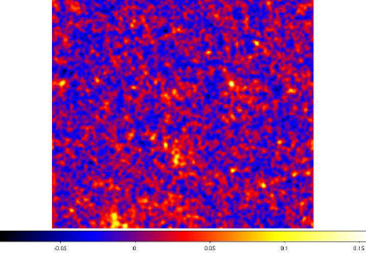
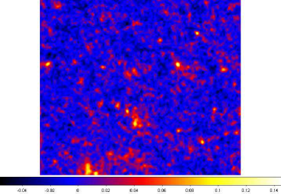
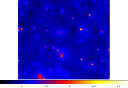
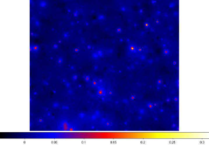
Figure 3: Noisy convergence maps of $3\times 3\hbox{ deg}^{2}$. The upper and lower panels are for the Gaussian smoothing with $\theta_{G}=1\hbox{ arcmin}$ and MRLens with $\alpha_{0}=0.01$, respectively. The left and right panels are for $n_{g}=30\hbox{ arcmin}^{-2}$ and $n_{g}=100\hbox{ arcmin}^{-2}$, respectively.

Comparing to the maps in Figure 1, we see that the post-processing procedures can indeed filter out much of the noise so that the real structures in the large-scale mass distribution can be detected. For $n_{g}=30\hbox{ arcmin}^{-2}$, the MRLens map looks very smooth with only very massive structures left. On the other hand, in the Gaussian smoothing case, small structures can also be seen. However, it contains many more noise peaks than that of the MRLens case. For $n_{g}=100\hbox{ arcmin}^{-2}$, the map is smoother for the Gaussian smoothing case than that with $n_{g}=30\hbox{ arcmin}^{-2}$. The MRLens map, however, appears lumpier for the lower noise case. Such opposite trends seen in the Gaussian smoothing and in MRLens reflect clearly the different underlying filtering mechanisms between the two smoothing schemes. For the Gaussian smoothing, the filtering is mainly performed through an averaging procedure. Given a smoothing scale, the peak signals of real clusters are more or less similar regardless the noise level. Meanwhile, the noise peaks with relatively high $\kappa$ values are significantly reduced if the noise level is lowered. Thus the smoother appearance of the upper right panel is mainly due to the less number of high noise peaks than that of the upper left panel. For MRLens, it involves a restoration procedure that depends on the original noise level. The smaller the original noise is, the lower the fraction is for the wavelet coefficients to be suppressed. It is important to note that the suppression leads to the removal of both noise peaks and true peaks of relatively low amplitudes. Thus the lumpier structures seen in the lower right panel is largely attributed to the lower level of removal of real structures than that of the lower left panel.

In Figure 4 and Figure 5, we show the probability distribution function of peaks for Gaussian smoothing and for MRLens, respectively. The results for each case are obtained by averaging over $16$ simulated maps with noise added.

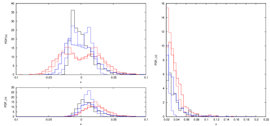
Figure 4: The probability distribution function of convergence peaks for the case of Gaussian smoothing with $\theta_{G}=1\hbox{ arcmin}$. The black solid line is for the result of the noise-free convergence peaks, the red dashed and red solid lines are for the pure noise peaks and noisy convergence peaks with $n_{g}=30\hbox{ arcmin}^{-2}$, respectively, and the blue dashed and blue solid lines are for the pure noise peaks and noisy convergence peaks with $n_{g}=100\hbox{ arcmin}^{-2}$, respectively. The left upper panel includes both maximum and minimum peaks, and the left lower panel shows the distribution function for maximum peaks only. The right panel is the zoom-in version of the left lower panel.

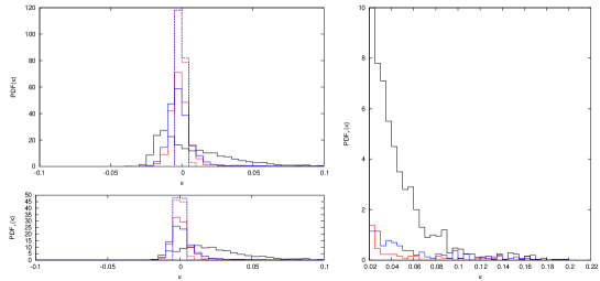
Figure 5: Same as Figure 4 but for the case of MRLens with $\alpha_{0}=0.01$.

For the Gaussian smoothing results in Figure 4, the black, red dashed, red solid, blue dashed, and blue solid lines are for the results of noise free peaks, pure noise peaks with $n_{g}=30\hbox{ arcmin}^{-2}$, noisy convergence peaks with $n_{g}=30\hbox{ arcmin}^{-2}$, pure noise peaks with $n_{g}=100\hbox{ arcmin}^{-2}$, noisy convergence peaks with $n_{g}=100\hbox{ arcmin}^{-2}$, respectively. We can see that in the Gaussian smoothing cases, the noise peaks dominate over the real peaks at $\kappa<3\sigma_{0}$. At larger $\kappa>3\sigma_{0}$, real peaks can be detected with high efficiencies. Comparing the blue solid line with the red solid line, we see that by reducing the noise level from $\sigma_{0}\sim 0.015$ to $\sigma_{0}\sim 0.008$, we effectively reduce the number of noise peaks with $\kappa>0.025$, and thus increase the real peak detection efficiencies significantly.

In Figure 5 for the MRLens results, the line styles are the same as those in Figure 4. Different from that in the Gaussian smoothing cases, here the noise peaks (red and blue dashed lines) contribute little to the total number of peaks with $\kappa>0.02$ in comparison with the real peaks (black solid line). However, the suppression process in the MRLens treatment mistakenly removes a large number of real peaks with $\kappa<0.1$. Thus we expect a high efficiency but a low completeness in weak-lensing peak detections after MRLens filtering. Reducing the original noise level by increasing $n_{g}$ form $30\hbox{ arcmin}^{-2}$ to $100\hbox{ arcmin}^{-2}$ leads to a less suppression effect. Therefore more peaks with $\kappa<0.1$ are kept and the completeness of peak detections increases considerably.

In the next subsection, we investigate and compare explicitly the efficiency and completeness of weak-lensing cluster detections in the two smoothing treatments.

4.3 Efficiency and completeness of weak-lensing cluster detection

The existence of noise from intrinsic ellipticities of source galaxies results false peaks in convergence maps, and thus lowers considerably the efficiency of weak-lensing cluster detections. Increasing the detection threshold can increase the efficiency, however at the expense of completeness. In this section, we compare the weak-lensing cluster detection with Gaussian smoothing and with the MRLens, respectively. Following Hamana et al. (2004), we define the efficiency $f_{e}$ and completeness $f_{c}$ of cluster detection with respect to the number of clusters (dark matter halos) above a certain mass threshold. Specifically, we have

$$f_{e}=\frac{N_{iii}}{N_{i}},$$ (31)

$$f_{c}=\frac{N_{iii}}{N_{ii}},$$ (32)

where $N_{i}$ denotes the number of convergence peaks with their heights above a detection threshold, $N_{ii}$ represents the number of dark matter halo with mass above a certain mass threshold, and $N_{iii}$ is the number of peaks that have correspondences with dark matter halos among $N_{ii}$. A peak is defined to be associated with its nearest dark matter halo if the location of the peak is within a radius of $12$ pixels (corresponds to $2.11\hbox{ arcmin}$) around the halo. If there are two or more peaks associated with a same halo, the highest peak is defined to have the correspondence with the halo.

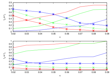
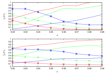
Figure 6: The efficiency $f_{e}$ and completeness $f_{c}$ as functions of the peak detection threshold $\kappa$. The left and right panels are for $n_{g}=30\hbox{ arcmin}^{-2}$ and $n_{g}=100\hbox{ arcmin}^{-2}$, respectively. The upper two panels are for the Gaussian smoothing and the lower two panels are for MRLens. The lines with symbols are for the completeness, and the lines without symbols are for the efficiency. The red, green and blue lines are for the results of halos with $M>5\times 10^{13}M_{\odot}$, $M>1\times 10^{14}M_{\odot}$, and $M>2\times 10^{14}M_{\odot}$, respectively.

Figure 6 shows the results of $f_{e}$ and $f_{c}$ for Gaussian smoothing (upper panels) and MRLens (lower panels). The left panels are for $n_{g}=30\hbox{ arcmin}^{-2}$, and the right panels are for $n_{g}=100\hbox{ arcmin}^{-2}$. In each panel, the red, green and blue lines are for halos with mass $M>5\times 10^{13}M_{\odot}$, $M>1\times 10^{14}M_{\odot}$, and $M>2\times 10^{14}M_{\odot}$, respectively. The lines with and without symbols are, respectively, for the results of completeness and efficiency. The horizontal axis in each panel is the peak detection threshold $\kappa$.

We first analyze the Gaussian smoothing cases. As we discuss previously, such a smoothing process reserves more or less all the real peaks with scales above the smoothing scale. At mean time, the number of noise peaks is large at $\kappa<3\sigma_{0}$. Thus a high completeness and a low efficiency are expected when the peak detection threshold is low. For $n_{g}=30\hbox{ arcmin}^{-2}$ (upper left), we have $\sigma_{0}\sim 0.015$. At the detection threshold $\kappa=0.02\sim 1.3\sigma_{0}$, we have the completeness $f_{c}\sim 50\%,65\%$ and $70\%$ for $M>5\times 10^{13}\hbox{ M}_{\odot}$, $1\times 10^{14}\hbox{ M}_{\odot}$ and $2\times 10^{14}\hbox{ M}_{\odot}$, respectively. The corresponding efficiencies are $30\%,10\%$ and $2\%$. When the detection threshold $\kappa>3\sigma_{0}$, the number of noise peaks drops significantly, leading to a large increase in the detection efficiency. On the other hand, a considerable fraction of halos are missed due to the high detection threshold, resulting a decrease in the completeness. Specifically, at $\kappa=0.045\sim 3\sigma_{0}$, the completeness $f_{c}\sim 20\%,35\%$ and $60\%$, and the efficiency $f_{e}\sim 50\%,25\%$ and $10\%$, for $M>5\times 10^{13}\hbox{ M}_{\odot}$, $1\times 10^{14}\hbox{ M}_{\odot}$ and $2\times 10^{14}\hbox{ M}_{\odot}$, respectively. With the increase of $n_{g}$ to $n_{g}=100\hbox{ arcmin}^{-2}$ (upper right), the noise level $\sigma_{0}$ decreases by a factor of $\sqrt{100/30}$ to $\sigma_{0}\sim 0.008$. Thus $3\sigma_{0}$ corresponds to $\kappa\sim 0.025$. At this detection threshold, the number of noise peaks is smaller and correspondingly the efficiency is higher than those with $n_{g}=30\hbox{ arcmin}^{-2}$. On the other hand, the number of real peaks does not change much as the noise level decreases, and thus the completeness is similar to that of $n_{g}=30\hbox{ arcmin}^{-2}$. Quantitatively, at the threshold $\kappa=0.025$, the efficiency $f_{e}\sim 50\%,20\%$ and $8\%$, in comparison with $f_{e}\sim 35\%,12\%$ and $3\%$ in the case of $n_{g}=30\hbox{ arcmin}^{-2}$, for $M>5\times 10^{13}\hbox{ M}_{\odot}$, $1\times 10^{14}\hbox{ M}_{\odot}$ and $2\times 10^{14}\hbox{ M}_{\odot}$, respectively. For the completeness, we have $f_{c}\sim 30\%,50\%$ and $80\%$ for $n_{g}=100\hbox{ arcmin}^{-2}$. For $n_{g}=30\hbox{ arcmin}^{-2}$, $f_{c}\sim 45\%,60\%$ and $70\%$. While being similar, $f_{c}$ decreases somewhat for $M>5\times 10^{13}\hbox{ M}_{\odot}$ and $1\times 10^{14}\hbox{ M}_{\odot}$ with the decrease of noise level. This is in accordance with the analyses of Fan et al. (2010) where they find that the existence of noise generates a systematic shift for the real peaks toward higher amplitudes. The shift depends on the density profile of dark matter halos associated with the real peaks, and can be as high as $\sim 1\sigma_{0}$ for NFW halos with low concentrations. In terms of $\kappa$ values, the shift is larger for larger $\sigma_{0}$. Thus, in the case of $n_{g}=30\hbox{ arcmin}^{-2}$, the relatively large $\sigma_{0}$ leads to a large shift of the real peak heights and consequently a larger number of real peaks above the detection threshold than that in the case of $n_{g}=100\hbox{ arcmin}^{-2}$.

For MRLens, with $n_{g}=30\hbox{ arcmin}^{-2}$ (lower left), the completeness of the weak-lensing cluster detection is very low, and $f_{c}\sim 10\%,20\%$ and $40\%$ at the threshold $\kappa=0.02$, in comparison with $f_{c}\sim 50\%,65\%$ and $70\%$ in the corresponding Gaussian smoothing case. This is because the suppression of the wavelet coefficients aiming to reduce noise removes a large fraction of real peaks in the range of $\kappa<0.1$ as seen from Figure 5. The total number of peaks in $3\times 3\hbox{ deg}^{2}$ with $\kappa\geq 0.02$ is only $\sim 53$, while the total number of halos in the area with $M>5\times 10^{13}\hbox{ M}_{\odot}$ is $\sim 530$. Thus although the efficiency in MRLens here is rather high ($\sim 80\%$ for $M>5\times 10^{13}\hbox{ M}_{\odot}$), the very few number of detected halos makes the MRLens method be disadvantageous in comparing with that of simple Gaussian smoothing method. For $n_{g}=100\hbox{ arcmin}^{-2}$, the noise level is lower and thus the removal effect is less significant than the case of $n_{g}=30\hbox{ arcmin}^{-2}$. Consequently, the completeness increases considerably with $f_{c}\sim 20\%,40\%$ and $65\%$. Meanwhile, the efficiency decreases somewhat. In this low noise case, the differences between the MRLens and Gaussian smoothing in terms of the completeness and efficiency are less than those of high noise case. But still, the completeness is lower for MRLens, especially considering relatively low mass halos with $M>5\times 10^{13}\hbox{ M}_{\odot}$.

To further demonstrate the differences between the Gaussian smoothing and the MRLens, in Figure 7, we show the peak-halo correspondences explicitly in $z-M$ plane for one of our $3\times 3\hbox{ deg}^{2}$ simulation maps, where $M$ is the halo mass in unit of $10^{13}M_{\odot}$ and $z$ is the halo redshift from simulations. The halos are the ones located in the solid angle of $3\times 3\hbox{ deg}^{2}$ in the considered direction and their redshift and mass are taken directly from the halo catalogs constructed by White and Vale (2004). The upper and lower panels are for the Gaussian smoothing and the MRLens, respectively. The left and right panels correspond to $n_{g}=30\hbox{ arcmin}^{-2}$ and $n_{g}=100\hbox{ arcmin}^{-2}$, respectively. In each panel, the ‘+’ symbols denote the dark matter halos identified in simulations with $M\geq 5\times 10^{13}M_{\odot}$ and in the redshift range of $0\leq z\leq 2$. There are very few halos extending to redshift beyond $z=2$. The green squares represent those halos that have corresponding convergence peaks with $\kappa\geq 0.02$. The differences between the two filtering methods are strikingly seen. For MRLens with $n_{g}=30\hbox{ arcmin}^{-2}$ (lower left), a majority of halos with $M<10^{14}\hbox{ M}_{\odot}$ or with $z>0.8$ are missed in weak-lensing detections, consistent with its extremely low completeness shown in Figure 6. Lowering the noise level by increasing $n_{g}$ to $n_{g}=100\hbox{ arcmin}^{-2}$ increases the number of halos with associated peaks by nearly a factor of $2$ (lower right). But the number is still much less than that in the Gaussian smoothing case. Therefore in studies aiming to detect a large number of clusters from blind surveys and subsequent cosmological applications, the Gaussian smoothing method is clearly much better than the MRLens. In addition, the noise field after a Gaussian smoothing with $\theta_{G}\sim 1\hbox{ arcmin}$ is approximately Gaussian in statistics, and thus its effects on weak-lensing cluster detection can be modeled much easier than the case of MRLens where the left-over noise is statistically highly non-Gaussian (Fan et al. 2010).

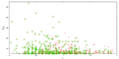
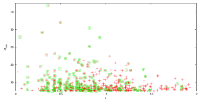
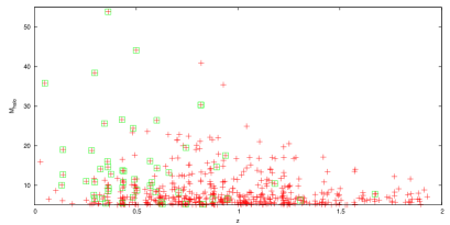
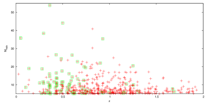
Figure 7: Peak-halo correspondences in $z-M$ plane. The upper and lower panels are for the Gaussian smoothing and MRLens, respectively. The left and right panels are for $n_{g}=30\hbox{ arcmin}^{-2}$ and $n_{g}=100\hbox{ arcmin}^{-2}$, respectively. In each panel, the ‘+’ symbols show all the halos with $M\geq 5\times 10^{13}M_{\odot}$ and the squares show the halos with corresponding convergence peaks with $\kappa\geq 0.02$.

In MRLens, the $\alpha_{0}$ parameter plays a crucial role in classifying significant and non-significant wavelet coefficients. A larger $\alpha_{0}$ leads to a larger fraction of significant coefficients, and thus a less suppression effect in MRLens restoration. To see if the problem of low completeness in MRLens cluster detection can be largely improved by increasing $\alpha_{0}$, we analyze the $\alpha_{0}$ dependence for the completeness $f_{c}$ as well as for the efficiency $f_{e}$. The results are shown in Figure 8. The upper and lower panels are for $n_{g}=30\hbox{ arcmin}^{-2}$ and $n_{g}=100\hbox{ arcmin}^{-2}$, respectively. The red, green and blue lines are for $M\geq 5\times 10^{13}M_{\odot}$, $1\times 10^{14}M_{\odot}$, and $2\times 10^{14}M_{\odot}$, respectively. The peak detection threshold is set to be $\kappa=0.02$. We can see that both $f_{c}$ and $f_{e}$ are not very sensitive to $\alpha_{0}$. Increasing $\alpha_{0}$ from $0.01$ to $0.1$ improves the completeness only by $\Delta f_{c}\sim 10\%$ for both $n_{g}=30\hbox{ arcmin}^{-2}$, and $n_{g}=100\hbox{ arcmin}^{-2}$. Meanwhile, the efficiency decreases by $\Delta f_{e}\sim 10\%-20\%$. Therefore increasing $\alpha_{0}$ cannot overcome the shortcoming of MRLens considerably. Comparing to the Gaussian smoothing cases, the completeness is still low for MRLens weak-lensing cluster detection even with $\alpha_{0}=0.1$.

We then conclude that in probing cosmologies with weak-lensing cluster abundance analyses, in which a large sample of clusters is needed, the Gaussian smoothing method performs much better than the MRLens method. To overcome the relatively low efficiency for low peaks in the Gaussian smoothing treatment, a detection threshold $\kappa>3\sigma_{0}$ is normally set. In Fan et al. (2010), the noise effects on convergence peak statistics can be accurately modeled for the Gaussian smoothing method. Therefore it is potentially possible to even include peaks with $\kappa<3\sigma_{0}$ in the abundance analyses, which can increase the number of detected clusters greatly so that to strengthen the derived cosmological constraints on different parameters. This will be explored further in our future studies.

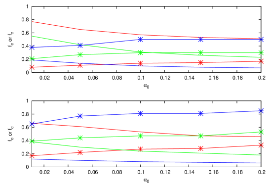
Figure 8: The $\alpha_{0}$ dependence of the completeness $f_{c}$ and the efficiency $f_{e}$. The upper and lower panels are for $n_{g}=30\hbox{ arcmin}^{-2}$ and $n_{g}=100\hbox{ arcmin}^{-2}$ respectively. The peak detection threshold is set to be $\kappa=0.02$. The red, green and blue lines are for the results of halos with $M>5\times 10^{13}M_{\odot}$, $M>1\times 10^{14}M_{\odot}$, and $M>2\times 10^{14}M_{\odot}$, respectively. The lines with and without symbols are for the completeness $f_{c}$ and the efficiency $f_{e}$, respectively.

5 Summary

Constructing cluster samples through their weak-lensing effects has been an important aspect of weak-lensing studies. Their statistical abundance contains valuable cosmological information. Observations have shown the feasibility in detecting clusters with weak-lensing effects (e.g., Wittman et al. 2006; Dietrich et al. 2007; Gavazzi & Soucail 2007; Schirmer et al. 2007; Hamana et al. 2009). In conjunction with optical observations, the detailed analyses on the completeness and efficiency of weak-lensing selected cluster samples also become possible (e.g., Geller et al. 2010). It is noted, however, the efficiency and completeness depend on the method applied to reconstruct the convergence field from shear measurements. Different methods can result residual noise with different statistical properties, and can also change the weak-lensing signals differently. In order to extract cosmological information from observations, it is therefore crucial to understand how a particular reconstruction method affects the results in detail.

In this paper, we systematically compare the Gaussian smoothing method and the MRLens treatment to suppress noise from intrinsic ellipticities in convergence maps. We concentrate on convergence peak statistics. It is found that while the MRLens method can remove noise very effectively, it mistakenly removes a large fraction of real peaks associated with clusters of galaxies. For $n_{g}=30\hbox{ arcmin}^{-2}$, the number of peaks with $\kappa\geq 0.02$ after MRLens filtering is only $\sim 50$ in an area of $3\times 3\hbox{ deg}^{2}$ in comparison with $\sim 530$ for the number of halos of $M>5\times 10^{13}\hbox{ M}_{\odot}$. On the other hand, for the Gaussian smoothing treatment, the number of detected clusters is $\sim 260$. Even with the detection threshold $\kappa=3\sigma_{0}\sim 0.045$, which is normally set in the Gaussian smoothing treatment to reduce the number of noise peaks in the peak catalog and thus to increase the cluster detection efficiency, the number of detected clusters is $\sim 100$, twice as many as that in the MRLens filtering with the threshold $\kappa=0.02$. As the accuracy of statistical abundance analyses depends crucially on the number of detected clusters, the Gaussian smoothing method is therefore strongly favored to detect clusters as many as possible. Furthermore, the Gaussian smoothing leads to a noise field which is approximately Gaussian in statistics, while the residual noise from MRLens filtering is highly non-Gaussian. Therefore the noise effects can be modeled more straightforwardly for the Gaussian smoothing case than that of MRLens (e.g., van Waerbeke 2000; Fan 2007; Fan et al. 2010). The recent studies of Fan et al. (2010) on the weak-lensing peak statistics with noise included provide an analytical model for the efficiency of peak detections in the Gaussian smoothing case. Thus it is possible for us to include peaks with $\kappa<3\sigma_{0}$ in the analyses. Then the number of detected clusters can increase considerably, which in turn can lead to a significant improvement in the cosmological constraints derived from weak-lensing cluster statistics.