On sub-ideal causal smoothing filters

Abstract

Smoothing causal linear time-invariant filters are studied for continuous time processes. The paper suggests a family of causal filters with almost exponential damping of the energy on the higher frequencies. These filters are sub-ideal meaning that a faster decay of the frequency response would lead to the loss of causality.
Key words: LTI filters, smoothing filters, casual filters, sub-ideal filters, Hardy spaces.
AMS 2010 classification : 42A38, 93E11, 93E10, 42B30

1 Introduction

The paper studies smoothing filters for continuous time processes. The consideration is restricted by the causal continuous time linear time-invariant filters (LTI filters), i.e. linear filters represented as convolution integrals over the historical data. These filters are used in dynamic smoothing, when the future values of the process are not available.

In the frequency domain, smoothing means reduction of the energy on the higher frequencies. In particular, an ideal low-pass filter is a smoothing filter. However, this filter is not causal, i.e., it requires the future value of the process. Moreover, a filter with exponential decay of the frequency response also cannot be causal [6]. It follows from the fact that a sufficient rate of decay of energy on higher frequencies implies some predictability of the processes; on the other hand, a causal filter cannot transform a general kind of a process into a predictable process. The classical result is Nyquist-Shannon-Kotelnikov interpolation theorem that implies that if a process is band-limited then it is predictable (see, e.g., [1]-[3],[5], [8]-[12], [15]-[18]). Recently, it was found that processes with exponential decay of energy on the higher frequencies are weakly predictable on a finite time horizon [6].

We suggest a family of causal smoothing filters with ”almost” exponential rate of damping the energy on the higher frequencies and with the frequency response that can be selected to approximate the real unity uniformly on an arbitrarily large interval. These filters are sub-ideal in the sense that their effectiveness in the damping of higher frequencies cannot be exceeded; a faster decay of the frequency response is not possible for causal filters. This is because this family of causal filters approximates the exponential decay rate of a reference set of non-causal filters (1).

2 Problem setting

Let $x(t)$ be a continuous-time process, $t\in{\bf R}$. The output of a linear filter is the process

$$y(t)=\int_{-\infty}^{\infty}h(t-\tau)x(\tau)d\tau,$$

where $h:{\bf R}\to{\bf R}$ is a given impulse response function.

If $h(t)=0$ for $t<0$, then the output of the corresponding filter is

$$y(t)=\int_{-\infty}^{t}h(t-\tau)x(\tau)d\tau.$$

In this case, the filter and the impulse response function are said to be causal. The output of a causal filter at time $t$ can be calculated using only past historical values $x(\tau)|_{\tau\leq t}$ of the currently observable continuous-time input process.

The goal is to approximate $x(t)$ by a smooth filtered process $y(t)$ via selection of an appropriate causal impulse response function $h(\cdot)$.

We are looking for families of the causal smoothing impulse response functions $h(\cdot)$ satisfying the following conditions.

• The outputs $y(\cdot)$ approximate processes $x(\cdot)$; the arbitrarily close approximation can be achieved by selection of an appropriate impulse response from the family.

• For processes $x(\cdot)\in L_{2}({\bf R})$, the outputs $y(\cdot)$ are infinitely differentiable functions. On the higher frequencies, the frequency response of the filter is as small as possible, to achieve the most effective damping of the energy on the higher frequencies of $x$.

• The effectiveness of this family in the damping of the higher frequencies cannot be exceeded; any faster decay of the frequency response would lead to the loss of causality.

• The effectiveness of this family in the damping of the higher frequencies approximates the effectiveness of some reference family of non-causal smoothing filters with a reasonably fast decay of the frequency response.

Note that it is not a trivial task to satisfy Conditions (C)-(D). For instance, consider a family of low-pass filters with increasing pass interval $[-\Delta,\Delta]$, where $\Delta>1$. Clearly, the corresponding smoothed processes approximate the original process as $\Delta\to+\infty$, i.e., Condition (A) is satisfied. However, the distance of the set of these ideal low-pass filters from the set of all causal filters is positive [1].

For $x(\cdot)\in L_{2}({\bf R})$, we denote by $X={\cal F}x$ the function defined on $i{\bf R}$ as the Fourier transform of $x(\cdot)$;

$$X(i\omega)=({\cal F}x)(i\omega)=\int_{-\infty}^{\infty}e^{-i\omega t}x(t)dt,\quad\omega\in{\bf R}.$$

Here $i=\sqrt{-1}$. For $x(\cdot)\in L_{2}({\bf R})$, the Fourier transform $X$ is defined as an element of $L_{2}({\bf R})$ (more precisely, $X(i\cdot)\in L_{2}({\bf R})$).

Consider a reference family of ”ideal” smoothing filters with the frequency response

$$M_{\mu}(i\omega)=e^{-\mu|\omega|},\quad\mu>0.$$ (1)

For these filters, Condition (A) is satisfied as $\mu\to 0$, and Conditions (B) is satisfied for all $\mu>0$. However, these filters are non-causal: for any $x(\cdot)\in L_{2}({\bf R})$, the output processes of these filters are weakly predictable at time $t$ on a finite horizon $[t,t+\mu)$ [6].

To satisfy Conditions (A)–(D), we consider a family of causal filters with impulse responses $\{h_{\nu}(\cdot)\}_{\nu=1}^{\infty}\subset L_{2}({\bf R})$ and with the corresponding Fourier transforms $H_{\nu}(i\omega)$, such that the following more special Conditions (a)-(d) are satisfied.

• Approximation of identity operator:

  (a1) For any $\Omega>0$, $H_{\nu}(i\omega)\to 1$ as $\nu\to+\infty$ uniformly in $\omega\in[-\Omega,\Omega]$.

  (a2) For any $x(\cdot)\in L_{2}({\bf R})$,

  $$\|y_{\nu}(\cdot)-x(\cdot)\|_{L_{2}({\bf R})}\to 0\quad\hbox{as}\quad\nu\to\infty,$$

  where $y_{\nu}$ is the output process

  $$y_{\nu}(t)=\int_{-\infty}^{t}h_{\nu}(t-\tau)x(\tau)d\tau.$$

• Smoothing property: For every $\nu>0$, there exists $\rho>0$ such that for any $n\geq 1$,

  $$\int_{-\infty}^{\infty}e^{|\omega|^{\rho}}|H_{\nu}(i\omega)|^{n}d\omega<+\infty.$$

• Sub-ideal smoothing: For any $\delta>1$, there exists $\nu>0$ such that for any $\Omega>0$

  $$\int_{\{\omega:\ |\omega|\geq\Omega\}}\frac{|\log|H_{\nu}(i\omega)||^{\delta}}{1+\omega^{2}}d\omega=+\infty.$$ (2)

• Approximation of non-causal filters (1) with respect to the effectiveness in damping: For any $\varepsilon>0$ and $\mu>0$, there exists $\nu=\nu(\mu)>0$ such that

  $$\bigl{\|}|H_{\nu}(i\omega)|-|M_{\mu}(i\omega)|\bigr{\|}_{L_{2}({\bf R})}\leq\varepsilon.$$

Let us show that Conditions (a)-(d) ensure that Conditions (A)-(D) are satisfied, in a certain sense. Clearly, Condition (a) ensures that Condition (A) is satisfied.

Further, by Condition (b), for any $k>0$ and $\nu>0$,

$$\int_{-\infty}^{\infty}(1+|\omega|^{k})^{4}|H_{\nu}(i\omega)|^{4}d\omega<+\infty.$$

Let $x(\cdot)\in L_{2}({\bf R})$, $X={\cal F}X$, and $Y_{\nu}(i\omega)=H_{\nu}(i\omega)X(i\omega)$. By Hölder inequality, it follows that

$$\int_{-\infty}^{\infty}(1+|\omega|^{k})^{2}|Y_{\nu}(i\omega)|^{2}d\omega\leq\left(\int_{-\infty}^{\infty}(1+|\omega|^{k})^{4}|H_{\nu}(i\omega)|^{4}d\omega\right)^{1/2}\|X\|_{L_{2}({\bf R})}^{1/2}<+\infty.$$

Hence $y_{\nu}(t)$ has derivatives in $L_{2}({\bf R})$ of any order, and, therefore, is infinitely differentiable in the classical sense. Therefore, Condition (b) ensures that Condition (B) is satisfied.

Let us show that Condition (c) ensures that Condition (C) is satisfied. Let $\delta>1$ be fixed, and let $\nu=\nu(\delta)$ be such that (2) holds. Let us show that the filter with the frequency response $\widetilde{h}={\cal F}^{-1}\widetilde{H}$ cannot be causal for some ”better” frequency response $\widetilde{H}(i\omega)$ such that

$$|\widetilde{H}(i\omega)|=o(|H_{\nu}(i\omega)|)\quad\hbox{as}\quad|\omega|\to+\infty.$$ (3)

More precisely, we will show that $\widetilde{h}$ cannot be causal with a stronger condition that there exists $\Omega>0$ such that

$$|\log|\widetilde{H}(i\omega)||\geq|\log|H_{\nu}(i\omega)||^{\delta},\quad|\omega|\geq\Omega.$$ (4)

In particular, this condition implies that $\log|H_{\nu}(i\omega)|/\log|\widetilde{H}(i\omega)|\to 0$ as $|\omega|\to+\infty$.

The desired fact that $\widetilde{h}$ cannot be causal can be seen from the following. By Paley and Wiener Theorem [14], the Fourier transform $H(i\omega)$ of a causal impulse response $h(\cdot)\in L_{2}({\bf R})$ has to be such that

$$\int_{-\infty}^{\infty}\frac{|\log|H(i\omega)||}{1+\omega^{2}}d\omega<+\infty$$

(see, e.g., [13], p.35). Since $\nu=\nu(\delta)$ is such that (2) holds, it follows from (4) that $\widetilde{h}$ cannot be causal. Therefore, Condition (c) ensures that Condition (C) is satisfied.

Finally, Condition (d) ensures that Condition (D) is satisfied, since the effectiveness of smoothing is defined by the rate of damping of the higher frequencies.

3 A family of sub-ideal smoothing filters

Let ${\bf C}^{+}\stackrel{{\scriptstyle{\scriptscriptstyle\Delta}}}{{=}}\{z\in{\bf C}:\ {\rm Re\,}z>0\}$. Let us consider a set of transfer functions

$$H_{a,b,q}(s)\stackrel{{\scriptstyle{\scriptscriptstyle\Delta}}}{{=}}e^{-a(s+b)^{q}},\quad s\in{\bf C}^{+}.$$ (5)

Here $a>0$, $b>0$, and $q\in[\bar{q},1)$, are rational numbers, $\bar{q}\in(0,1)$ is a given number. We mean the branch of $(s+b)^{q}$ such that its argument is $q{\rm Arg\,}(s+b)$, where ${\rm Arg\,}z\in(-\pi,\pi]$ denotes the principal value of the argument of $z\in{\bf C}$. This set was introduced in [4] as an auxiliary tool for solution of a parabolic equation in the frequency domain.

Let us consider the set of all transfer functions (5) with rational numbers $a>0$, $b>0$, and $q\in[1/2,1)$. We assume that this countable set is counted as a sequence $\{H_{\nu}\}_{\nu=1}^{\infty}$ such that $a\to 0$, $b\to 0$, $q\to 1$ as $\nu\to+\infty$.

Theorem 1

Conditions (a)-(d) are satisfied for the family of filters defined by the transfer functions $\{H_{\nu}\}_{\nu=1}^{\infty}$. (Therefore, Conditions (A)-(D) are satisfied for this family).

Proof of Theorem 1. Let $H^{r}$ be the Hardy space of holomorphic on ${\bf C}^{+}$ functions $h(p)$ with finite norm $\|h\|_{H^{r}}=\sup_{\rho>0}\|h(\rho+i\omega)\|_{L_{r}({\bf R})}$, $r\in[1,+\infty]$ (see, e.g., [7]).

Clearly, the functions $H_{\nu}(p)$ are holomorphic in ${\bf C}^{+}$, and

$$\ln|H_{\nu}(s)|=-{\rm Re\,}(a(s+b)^{q})=-a|s+b|^{q}\cos[q{\rm Arg\,}(s+b)].$$ (6)

In addition, there exists $M=M(b,q)>0$ such that $\cos[q{\rm Arg\,}(p+b)]>M$ for all $s\in{\bf C}^{+}$. It follows that

$$|H_{\nu}(s)|\leq e^{-aM|s+b|^{q}}<1,\quad s\in{\bf C}^{+}.$$ (7)

Hence $H_{\nu}\in H^{r}$ for all $r\in[1,+\infty]$. By Paley-Wiener Theorem, the inverse Fourier transforms $h_{\nu}={\cal F}^{-1}H_{\nu}(i\omega)$ are causal impulse responses, i.e., $h_{\nu}(t)=0$ for $t<0$ (see, e.g., [19], p.163).

Let $x\in L_{2}({\bf R})$, $X={\cal F}x$, and $Y_{\nu}=H_{\nu}X$.

Let us show that Condition (a) holds. Since $a\to 0$ as $\nu\to+\infty$, it follows that $H_{\nu}(i\omega)\to 1$ as $\nu\to+\infty$ for any $\omega$ and that Condition (a1) holds. By Condition (a1), $Y_{\nu}(i\omega)\to X(i\omega)$ as $\nu\to+\infty$ for all $\omega\in{\bf R}$. In addition, $|H_{\nu}(i\omega)|\leq 1$. Hence $|Y_{\nu}(i\omega)-X(i\omega)|\leq 2|X(i\omega)|$. We have that $\|X(i\omega)\|_{L_{2}({\bf R})}=\|x\|_{L_{2}({\bf R})}<+\infty$. By Lebesgue Dominance Theorem, it follows that

$$\left\|Y_{\nu}(i\omega)-X(i\omega)\right\|_{L_{2}({\bf R})}\to 0\quad\hbox{as}\quad\nu\to+\infty.$$

Therefore, Condition (a) holds.

Let us show that Condition (b) holds. By (7), it follows that

$$|H_{\nu}(i\omega)|\leq e^{-aM|\omega|^{q}},\quad\omega\in{\bf R}.$$ (8)

Therefore, Condition (b) holds with any $\rho<q$.

To see that Condition (c) holds, it suffices to observe that (2) holds if $\delta q\geq 1$, i.e., $q\geq 1/\delta$.

Let us show that Condition (d) holds. We assume that the family of transfer functions $H_{a,b,q}(\cdot)$ is counted as a sequence $\{H_{\lambda}\}_{\lambda=1}^{\infty}$ such that $b\to 0$, $q\to 1$ as $\lambda\to+\infty$, with $a=\mu/\cos(q\pi/2)$. We have that $\cos[q{\rm Arg\,}(i\omega+b)]\geq\cos(q\pi/2)$ for all $b>0$, $\omega\in{\bf R}$ and $\cos[q{\rm Arg\,}(i\omega+b)]\to\cos(q\pi/2)$ as $b\to 0$ for all $q\leq 1$, $\omega\in{\bf R}$.

By (6), $|H_{\lambda}(i\omega)|\to|M_{\mu}(i\omega)|$ as $\lambda\to+\infty$ for all $\omega\in{\bf R}$. Further, we have that

$$-\ln|H_{\lambda}(i\omega)|=a{\rm Re\,}[(i\omega+b)^{q}]=a|i\omega+b|^{q}\cos[q{\rm Arg\,}(i\omega+b)]$$

$$\geq a|i\omega+b|^{q}\cos(q\pi/2)\geq a|\omega|^{q}\cos(q\pi/2).$$ (9)

Hence $-\ln|H_{\lambda}(i\omega)|\geq\mu|\omega|^{q}$ and $|H_{\lambda}(i\omega)|\leq e^{-\mu|\omega|^{q}}.$ Since $q\geq\bar{q}>0$, we have from (8) that, for some constants $c_{1}>0$ and $c_{2}>0$, $|H_{\lambda}(i\omega)|+|M_{a}(i\omega)|\leq c_{1}\exp\left(-c_{2}(|\omega|^{\bar{q}}+|\omega|)\right)$ for all $\omega$. By Lebesgue Dominance Theorem, it follows that

$$\bigl{\|}|H_{\lambda}(i\omega)|-|M_{\mu}(i\omega)|\bigr{\|}_{L_{2}({\bf R})}\to 0\quad\hbox{as}\quad\lambda\to+\infty.$$ (10)

Hence Condition (d) holds. This completes the proof of Theorem 1. $\Box$

Note that the sequence $H_{\lambda}(s)$ introduced above does not ensure approximation described by Condition (a1), since $a\to+\infty$ and $H_{\lambda}(0)\to 0$ as $\lambda\to+\infty$. On the other hand, the sequence $H_{\nu}(s)$ does not ensure approximation (10). The following corollary shows a way toward the combination of these approximation properties.

Corollary 1

Let $q\in[\bar{q},1)$ and $b>0$ be given. Let a sequence $\{H_{n}(\cdot)\}=\{H_{a,b,q}(\cdot)\}$ be selected such that $a\to 0$. Then Condition (a1) holds for this sequence, and $|H_{n}(i\omega)|\leq e^{-c|\omega|^{q}}$ for all $\omega$, where $c=a\cos(q\pi/2)$.

Proof of Corollary 1 follows from (9).

4 Illustrative examples

The sequence $\{H_{\lambda}(\cdot)\}$ introduced in the proof above is such that $\||H_{\lambda}(i\omega)|-\exp(-\mu|\omega|)\|_{L_{2}({\bf R})}\to 0$ as $\lambda\to+\infty$, i.e., it approximates the gain of the non-causal smoothing filter with the frequency response $M_{\mu}(i\omega)=\exp(-\mu|\omega|)$. This sequence corresponds to a sequence $\{H_{a,b,q}(\cdot)\}$ such that $q\to 1$, $b\to 0$, $a=\mu/\cos(q\pi/2)$. Figure 1 shows the shapes of gain curves $|M_{\mu}(i\omega)|=\exp(-\mu|\omega|)$ for the reference non-causal filter with $\mu=0.1$ and $|H_{a,b,q}(i\omega)|$ for sub-ideal causal filters (5) with $q=0.99$ and $b=1-q=0.01$ and $q=0.9$, $b=1-q=0.1$ respectively. In both cases, $a=\mu/\cos(q\pi/2)$ was used. As expected, damping on higher frequencies is more effective for the non-causal filter than for causal ones, and is more effective for $q=0.99$ than for $q=0.9$. It can be illustrated as the following: for $\omega=1000$, the ratio $\frac{|H_{a,b,q}(i\omega)|}{|M_{\mu}(i\omega)|}$ is found to be 1.47 and 38.65 for $q=0.99$ and $q=0.9$ respectively.

Figure 2 illustrates Corollary 1 and shows the shapes of error curves for approximation of identity operator on low frequencies. More precisely, it shows $|M_{\mu}(i\omega)-1|=\left|e^{-\mu|\omega|}-1\right|$ for the reference non-causal filter with $\mu=0.05$ and $|H_{a,b,q}(i\omega)-1|$ for sub-ideal causal filters (5) with $a=b=0.1$ and $a=b=0.05$ respectively, with $q=0.5$.

Figure 3 shows an example of impulse response $h_{a,b,q}(t)=({\cal F}^{-1}H_{a,b,q})(t)$ calculated as the inverse Fourier transform for causal filter (5) with $q=0.9$, $b=0.1$, $a=1/\cos(q\pi/2)=6.3925$. It can be seen that the impulse response function almost vanishes on some interval near zero, i.e., it is close to a causal impulse response with delay. (However, it does not become a response with delay). There is a reason for this: if $q\to 1$ and $b\to 0$ then, for a given $a,c>0$, $H_{a,b,q}(p)\to e^{ap}$ uniformly in the domain $\{p\in{\bf C}^{+}:|p|\leq c\}$.

It can be noted that the phase shift for the frequency response function is large for large $|\omega|$, and it is increasing when $q\to 1$. This does not affect much the performance of the filter since the gain is small for these large $|\omega|$ and Condition (a1) is ensured.

5 Conclusion

The paper proposes a family of causal smoothing filters with almost exponential damping of the energy on the higher frequencies and with the frequency response that can be selected to be arbitrarily close to the real unity uniformly on an arbitrarily large interval. These filters are sub-ideal meaning that a faster decay of the frequency response would lead to the loss of causality; this is because they approximate non-causal filters with exponential rate of decay. A possible application is in interpolation and forecast algorithms. The transfer functions obtained are not rational functions; it would be interesting to consider their approximation by the rational functions. Another problem is the transition to discrete time processes. We leave it for future research.

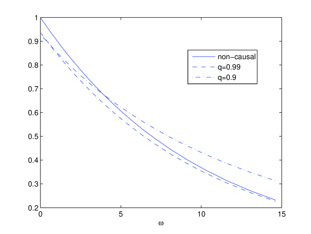
Figure 1: Gain decay: shapes of $|M_{\mu}(i\omega)|=\exp(-\mu|\omega|)$ for non-causal filter with $\mu=0.1$ and $|H_{a,b,q}(i\omega)|$ for causal filters (5) with $q=0.99$, $b=0.01$ and $q=0.9$, $b=0.1$ respectively, with $a=\mu/\cos(q\pi/2)$.

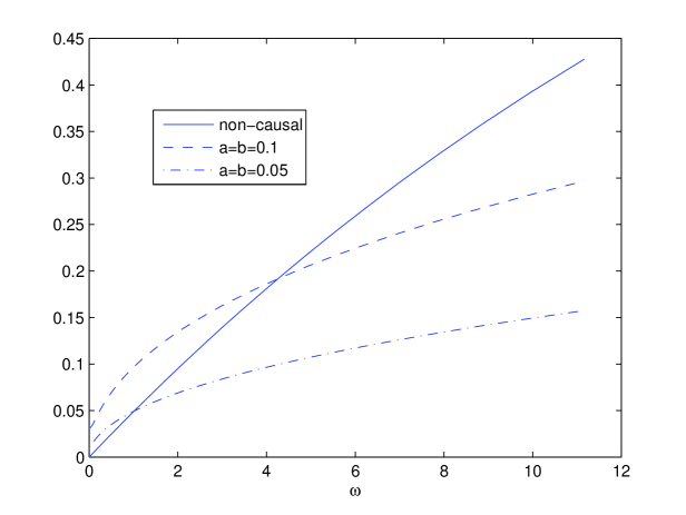
Figure 2: Approximation of identity operator: shapes of error curves $|M_{\mu}(i\omega)-1|$ and $|H_{a,b,q}(i\omega)-1|$ respectively for non-causal filter with $\mu=0.05$ and for causal filters (5) with $a=b=0.1$ and $a=b=0.05$, with $q=0.5$.

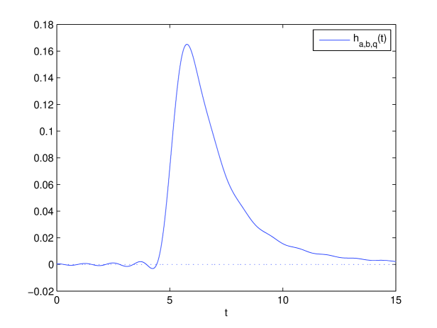
Figure 3: Impulse response $h_{a,b,q}(t)=({\cal F}^{-1}H_{a,b,q})(t)$ for causal filter (5) with $q=0.9$, $b=0.1$, $a=1/\cos(q\pi/2)=6.3925$.

References

- [1] J.M. Almira and A.E. Romero. How distant is the ideal filter of being a causal one? Atlantic Electronic Journal of Mathematics 3 (1) (2008) 46–55.
- [2] F.G. Beutler. Error-free recovery of signals from irregularly spaced samples, SIAM Review 8 (3) (1966) 328–335.
- [3] J.R. Brown Jr. Bounds for truncation error in sampling expansion of band-limited signals, IEEE Transactions on Information Theory 15 (4) (1969) 440-444.
- [4] N. Dokuchaev. Parabolic equations with the second order Cauchy conditions on the boundary, Journal of Physics A: Mathematical and Theoretical 40 (2007) 12409–12413.
- [5] N. Dokuchaev. The predictability of band-limited, high-frequency, and mixed processes in the presence of ideal low-pass filters, Journal of Physics A: Mathematical and Theoretical 41 (2008) 382002 (7pp).
- [6] N. Dokuchaev. Predictability on finite horizon for processes with exponential decrease of energy on higher frequencies, Signal processing 90 (2) (2010) 696–701.
- [7] P. Duren. Theory of -Spaces. Academic Press, New York, 1970.
- [8] J.R. Higgins. Sampling Theory in Fourier and Signal Analysis. Oxford University Press, NY, 1996.
- [9] J.J. Knab. Interpolation of band-limited functions using the approximate prolate series, IEEE Transactions on Information Theory 25 (6) (1979) 717–720.
- [10] R.J. Lyman, W.W. Edmonson, S. McCullough, and M. Rao. The predictability of continuous-time, bandlimited processes, IEEE Transactions on Signal Processing 48 (2) (2000) 311–316.
- [11] R.J. Lyman and W.W. Edmonson. Linear prediction of bandlimited processes with flat spectral densities, IEEE Transactions on Signal Processing 49 (7) (2001) 1564–1569.
- [12] F. Marvasti. Comments on ”A note on the predictability of band-limited processes”, Proceedings of the IEEE 74 (11) (1986) 1596.
- [13] L.D. Paarmann. Design and analysis of analog filters. A signal processing perspective with MatLab examples. Kluwer Academic Publishers, NY, 2003.
- [14] R.E.A.C. Paley and N. Wiener. Fourier transforms in the complex domain, Amer. Math. Soc. Colloquium Publications XIX (1934).
- [15] A. Papoulis. A note on the predictability of band-limited processes, Proceedings of the IEEE 73 (8) (1985) 1332–1333.
- [16] D. Slepian. Prolate spheroidal wave functions, Fourier analysis, and uncertainty–V: The discrete case, Bell System Technical Journal, 57 (5) (1978) 1371–1430.
- [17] P.P. Vaidyanathan. On predicting a band-limited signal based on past sample values, Proceedings of the IEEE 75 (8) (1987) 1125–1127.
- [18] L.A. Wainstein and V.D. Zubakov. Extraction of Signals from Noise. Prentice Hall, Englewood Cliffs, NJ, 1962.
- [19] K. Yosida, Functional Analysis. Springer, Berlin Heilderberg New York, 1965.