Comments on k-Strings at Large N

Abstract

We present a computation of the k-string tension in the large N limit of the two-dimensional lattice Yang-Mills theory. It is well known that the problems of computing the partition function and the Wilson loop can be both reduced to a unitary matrix integral which has a third order phase transition separating weak and strong coupling. We give an explicit computation of the interaction energy for $k$-strings in the large $N$ limit when $\tfrac{k}{N}$ is held constant and non-zero. In this limit, the interaction energy is finite and attractive. We show that, in the strong coupling phase, the $k\to N-k$ duality is realized as a first order phase transition. We also show that the lattice $k$-string tension reduces to the expected Casimir scaling in the continuum limit.

K-string tension has been proposed as an interesting probe of the confining phase of Yang-Mills theory [1][2][3][4][5][6][7][8][9][10]. In the dual superconductor picture of confinement, lines of electric flux which emanate from a source with color charge are confined to flux tubes, the confining strings. If a colored source has center-charge $k$, it is the endpoint of $k$ flux tubes. There is immediately an interesting question as to whether these flux tubes attract and perhaps bind together to form a single tube with $k$ units of flux, or whether they repel each other and tend to remain as individual vortices, that is whether the dual superconductor is of type I or type II, respectively.

In Yang-Mills theory, or any gauge theory with only adjoint (or other center-neutral) matter, the k-string tension $\sigma_{k}$ is defined as

$$e^{-\sigma_{k}A}=\frac{1}{{\rm dim}{\cal A}_{k}}\left<{\rm Tr}_{{\cal A}_{k}}e^{i\oint_{C}A_{\mu}dx^{\mu}}\right>~{},$$ (1)

where $C$ is typically a rectangular loop with dimensions $L\times T$, $A=LT$ is the area subtended by that loop and ${\cal A}_{k}$ is the irreducible representation of the gauge group where the Young tableau consists of a single column of $k$ boxes, depicted in Fig. 1. We are assuming that the gauge group is $SU(N)$. The physical interpretation of (1) lies in the idea that, if we introduce a heavy $k$-quark and a heavy anti-$k$-quark separated a distance $L$ much greater than the confinement scale into the confining phase of Yang-Mills theory, the energy attributable to the gauge theory mediated interaction between them is $E=\sigma_{k}L$. The linear growth of the energy with distance is a signal of confinement. The coefficient $\sigma_{k}$ is a measure of the strength of the confining interaction.

${\Young~{}\cr~{}\cr~{}\cr~{}\cr~{}\cr~{}\cr~{}\cr}$

Figure 1: The Young tableau corresponding to a completely antisymmetric representation ${\cal A}_{k}$ of SU(N) consists of a single column with $k$ boxes.

An intuitive way of thinking about the $k$-string is to imagine that we bring $k$ confining strings close to each other. If these elementary strings have an attractive interaction, $\sigma_{k}<k\sigma_{1}$, and the strings can from a bound state which we call the $k$-string. The $k$-string tension is not easily accessible to perturbation theory and, aside from some supersymmetric models where exact results can be obtained [11], it is most readily studied by numerical simulations of lattice gauge theory. In this Letter, we will study it in a solvable model, the large $N$ limit of two-dimensional Yang-Mills theory that was originally formulated and solved by Gross and Witten [12]. The fundamental and adjoint Wilson loops in this model have been used as models of deconfinement transitions in finite temperature Yang-Mills theory Khokhlachev:1979tx[14][15].

If we were to consider an expectation value of a Wilson loop as in (1), but taken in some other representation of the gauge group where the Young tableau also has $k$ boxes, the expectation value should turn out to be independent of the representation and equal to that obtained for a k-string in the completely antisymmetric representation ${\cal A}_{k}$. This is because we expect the color charge of the quarks to be screened by the gluons which, since they are center charge neutral, conserve the center charge $k$ but, by combining with the strings of electric flux, can alter the precise representation. This screening is not expected to occur in two dimensions where there are no dynamical gluons. It is also not expected to occur in the large $N$ limit where large $N$ factorization means that mixing of representations is suppressed by factors of $\tfrac{1}{N}$. Lack of mixing of representations would lead us to expect that in two dimensions, or at large $N$, the k-string tension is always given by the weak coupling result, $\sigma_{k}=k\sigma_{1}$. At a first glance, large $N$ factorization would suggest that the interaction energy of a $k$-string, $\sigma_{k}-k\sigma_{1}$, should be of order $\tfrac{1}{N^{2}}$ in the ’t Hooft large $N$ expansion, and therefore vanishingly small in the large $N$ limit. However, since at infinite $N$ all representations have the same tension, lifting the degeneracy at finite $N$ can lead to corrections of order $1/N$, as we will see shortly . There are lattice simulations which suggest that corrections to the $k$-string tension in $3$ dimensions indeed scale like $\tfrac{1}{N}$, rather than $\tfrac{1}{N^{2}}$ [10]. In addition, the lattice simulations seem to indicate that the splitting of the energies of representations with the same center charge is identifiable, is also of order $\tfrac{1}{N}$ and is unexpectedly small.

The $k$-string tension is expected to be symmetric under the replacement of $k$ by $N-k$ so that

$$\sigma_{k}=\sigma_{N-k}~{}.$$ (2)

This is obtained by replacing probe quarks by anti-quarks and vice-versa. In contrast, weak coupling implies that $\sigma_{k}\approx k\sigma_{1}$. While this fundamental $k\rightarrow N-k$ symmetry is compatible with $k$-strings being weakly coupled for $k\ll N$, since $k$ and $N-k$ cannot both be much less than $N$, in the regime where $N$ is large and $k\sim N$, $k$-strings cannot be weakly interacting.

Continuum Yang-Mills theory in two dimensions is solvable and the $k$-string tension is known exactly,

$$\sigma_{k}^{D=2}=\lambda C_{2}({\cal R}_{k})~{},$$ (3)

where $\lambda=g^{2}N$ is the ’t Hooft coupling and $g$ is the Yang-Mills theory coupling constant. $C_{2}(R)$ is the quadratic Casimir operator of the representation ${\cal R}_{k}$. As expected, because there are no dynamical gluons, the string tension is not independent of representation. For a completely antisymmetric representation ${\cal A}_{k}$, it is

$$C_{2}({\cal A}_{k})=\tfrac{k(N-k)}{N}~{}.$$ (4)

This expression is symmetric under the replacement $k\to N-k$. This $k$-string tension has $\sigma_{k}^{D=2}=k\sigma_{1}^{D=2}-\tfrac{k^{2}}{N}\sigma_{1}^{D=2}$, the first term interpreted as the energy of $k$ non-interacting fundamental strings and the second term being the interaction energy. Thus, the interaction between $k$-strings in two dimensions seems to be attractive when they are in the antisymmetric representation. It is also easy to see that for expectation values of a Wilson loop in other representations, the interaction energy can be repulsive.

The Casimir scaling hypothesis is that the $k$-string tension in higher dimensions remains proportional to $C_{2}({\cal A}_{k})$, dependent on the center charge $k$ but, because of screening, otherwise independent of the representation of the probe quarks. This hypothesis is seemingly contradicted by the sine-law: an alternative, first principles result found in softly broken ${\cal N}=2$ supersymmetric Yang-Mills theory [11] where the $k$-string is a BPS object

$$\sigma_{k}=m\Lambda N\sin\tfrac{\pi k}{N}~{}.$$ (5)

The sine-law is consistent with results found in MQCD [16] and AdS/CFT [17]. One interesting difference between the Casimir scaling and sine-law behaviors is that the corrections to the leading order in the large $N$ limit of Casimir scaling are of order $1/N$ whereas for the sine-law they are of order $1/N^{2}$. In both cases, though, k-strings are strongly interacting when $k\sim N$ as was discussed above.

In the following, we shall find a third expression for the $k$ string tension which follows from the large $N$ limit of two dimensional lattice Yang-Mills theory. Above, we have pointed out two non-generic features of the $k$-string in two dimensions and at large $N$. One is the absence of dynamical gluons in two dimensions which leads to representation dependence, as is already seen, for example, in the continuum formula (3). The other is the absence of mixing of representations which happens in the large $N$ limit in any dimensions, so that $k$-strings are non-interacting. In the following, we shall find a way to circumvent the second shortcoming by studying representations with center charge $k$ where $k\sim N$. As has been discussed, this is not compatible with weak coupling; mixing of representations, which would be suppressed by powers of $\tfrac{k}{N}$, is allowed and is of unit magnitude when $k\sim N$. Since the interaction is not suppressed by a power of $\tfrac{1}{N}$, one question that our computation can answer is whether confining strings continue to have an attractive interaction so that $k$-strings are stable when the interaction is strong. We shall find that it is indeed attractive and $\sigma_{k}-k\sigma_{1}$ is negative for all values $0<\tfrac{k}{N}<1$. We shall also confirm that the string tension in the two-dimensional model indeed depends on the representation and, for the completely symmetric representation with center charge $k$, the interaction between confining strings is repulsive for all values of $\tfrac{k}{N}>0$.

A Wilson loop in the two dimensional lattice Yang-Mills theory is computed by the integral

$$W_{\cal R}[C]=\frac{\int\prod_{\ell}[dU_{\ell}]e^{\tfrac{N}{\lambda}\sum_{P}{\rm Tr}\left(\prod_{\ell\in\delta P}U_{\ell}+\prod_{\ell\in\delta P}U^{\dagger}_{\ell}\right)}~{}\frac{1}{{\rm dim}{\cal R}}{\rm Tr}_{\cal R}\prod_{\ell\in C}U_{\ell}}{\int\prod_{\ell}[dU_{\ell}]e^{\tfrac{N}{\lambda}\sum_{P}{\rm Tr}\left(\prod_{\ell\in\delta P}U_{\ell}+\prod_{\ell\in\delta P}U^{\dagger}_{\ell}\right)}}$$ (6)

where $P$ and $\ell$ label plaquettes and links, respectively, of a square lattice, $U_{\ell}$ is a unitary matrix residing on the links, $[dU_{\ell}]$ is the invariant Haar integration measure for $SU(N)$, ${\cal R}$ is an irreducible representation and ${\rm Tr}_{\cal R}$ is the character in that representation. This model was first solved in the large $N$ limit by Gross and Witten [12]. Using the gauge fixing of Ref. [12] and the Peter-Weyl theorem $\int[dU]U_{ij}^{\cal R}U_{kl}^{\dagger{\cal R}^{\prime}}=\tfrac{\delta_{il}\delta_{jk}\delta_{{\cal R}{\cal R}^{\prime}}}{{\rm dim}{\cal R}}$, it is possible to reduce this to a one-plaquette unitary matrix model [18]

$$W_{\cal R}[C]~{} =~{}\left[w_{\cal R}[C]\right]^{A}~{}=~{}e^{-\sigma_{\cal R}A}~{},$$

$$\sigma_{\cal R}~{} =~{}-\ln\left[~{}\frac{\int[dU]e^{\tfrac{N}{\lambda}{\rm Tr}\left(U+U^{\dagger}\right)}~{}\frac{1}{{\rm dim}{\cal R}}\left[{\rm Tr}_{\cal R}U\right]}{\int[dU]e^{\tfrac{N}{\lambda}{\rm Tr}\left(U+U^{\dagger}\right)}}\right]~{},$$ (7)

where $A$ is the area of the loop – the number of plaquettes in an area that is bounded by the loop – and the string tension $\sigma_{{\cal R}}$ is measured in units of inverse lattice spacing squared. Note that the Wilson loop in the one plaquette model is normalized by the dimension of the representation. This is a result of repeated use of the Peter-Weyl theorem when reducing to the one-plaquette model. It has the important consequence that, since in this simple one-matrix model, the dimension of the representation is the upper bound on the expectation value of the character of a matrix in that representation, the string tension is always positive and the gauge theory interaction is always confining.

The one-plaquette model which computes $\sigma_{\cal R}$ in (7) is solvable in the large $N$ limit. Gauge invariance allows one to diagonalize $U={\rm diag}\left(e^{i\phi_{1}},\ldots,e^{i\phi_{N}}\right)$ and the remaining integral over eigenvalues can be done in the saddle-point approximation where the resulting action is of order $N^{2}$, so that fluctuations are suppressed by powers of $\tfrac{1}{N^{2}}$. The classical configuration of the eigenvalues is determined by minimizing the action plus a term arising from the integration measure. In all of the cases that we shall consider, if we seek only the leading order in large $N$, the loop inserted into (7) can be treated as a probe where the expectation value is evaluated simply by plugging in the classical distribution of eigenvalues that is determined by the action. This distribution is characterized by the eigenvalue density, defined as the large $N$ limit of $\rho(\phi)=\tfrac{1}{N}\sum_{i}\delta(\phi-\phi_{i})$. The model (7) has a third order phase transition when $\lambda=2$. The two phases have eigenvalue densities [12]

$$\rho(\phi) = ~{}\tfrac{1}{2\pi}\left(1+\tfrac{2}{\lambda}\cos\phi\right)~{},~{}\textrm{for}~{}\lambda>2~{},$$ (8)

$$\rho(\phi) = ~{}\tfrac{2}{\pi\lambda}\cos\tfrac{\phi}{2}\sqrt{\tfrac{\lambda}{2}-\sin^{2}\tfrac{\phi}{2}}~{},~{}\textrm{for}~{}0<\lambda<2~{},$$ (9)

where, in (9), $|\phi|<2\arcsin\sqrt{\tfrac{2}{\lambda}}$ and on the remainder of the circle $\rho=0$.

The easiest representations to consider are the totally antisymmetric ${\cal A}_{k}$ whose Young tableau consists of a single column of $k$ boxes and the totally symmetric ${\cal S}_{k}$ whose Young tableau is a row with $k$ boxes. The analysis of the symmetric representation in a unitary one-matrix model was explained in detail in Ref. [19] and we will refer the reader there for the details. Here, we will concentrate on the antisymmetric representation, corresponding to a k-string.

In terms of eigenvalues, the symmetry can be used to order the indices in the trace so that they are non-decreasing

$${\rm Tr}_{{\cal A}_{k}}U=\sum_{a_{1}<\ldots<a_{k}}e^{i\phi_{a_{1}}}e^{i\phi_{a_{2}}}\ldots e^{i\phi_{a_{k}}}~{}.$$ (10)

It is convenient to obtain this expressions from a generating function [20][19]

$${\rm Tr}_{{\cal A}_{k}}U=\oint\frac{dt}{2\pi it^{k+1}}\prod_{a=1}^{N}\left(1+te^{i\phi_{a}}\right)~{},$$ (11)

where the contour integral projects onto the term in a Taylor expansion of the integrand which contains $k$ eigenvalues. The covariant expression is

$$\langle{\rm Tr}_{{\cal A}_{k}}~{}U\rangle~{}=~{}\oint\frac{dt}{2\pi it^{k+1}}\langle\exp\left[{\rm Tr}\ln(1+tU)\right]\rangle~{}.$$ (12)

In the large $N$ limit, the traces in the exponents in the above equations are replaced by integrals over the eigenvalue densities (8) or (9):

$$\langle{\rm Tr}_{{\cal A}_{k}}~{}U\rangle~{}=~{}\oint\frac{dt}{2\pi it^{k+1}}\exp\left[N\int d\phi\rho(\phi)\ln(1+te^{i\phi})-k\ln t\right]~{}.$$ (16)

When $k$ is large, we can use the saddle-point approximation to evaluate the integral over $t$ in (12). Let $\hat{t}$ satisfy the saddle-point equation

$$R_{{\cal A}_{k}}(\hat{t})\equiv\int_{-\pi}^{\pi}d\phi\rho(\phi)\frac{\hat{t}e^{i\phi}}{1+\hat{t}e^{i\phi}}=\frac{k}{N}~{}.$$ (17)

The functions $R_{{\cal A}_{k}}(t)$ in (17) are related to the resolvent of the matrix model and are holomorphic functions of $t$ with cut singularities on the unit circle determined by the support of $\rho(\phi)$. With the strong coupling phase (8), $\lambda>2$, the cut singularity on the left-hand-side of (17) occupies the entire unit circle and divides the plane into two regions, the interior and the exterior of the unit circle. We extend each of these regions to disjoint Riemann sheets, each of which covers the entire plane. We then search for solutions of the saddle-point equations on each of these sheets. The saddle-point equations for each of the two sheets are

$$\tfrac{1}{\lambda}\hat{t} = \tfrac{k}{N}~{},$$ (18)

$$1-\tfrac{1}{\lambda}\frac{1}{\hat{t}} = \tfrac{k}{N}~{}.$$ (19)

and the solutions are

$$\hat{t}_{1} = \lambda\tfrac{k}{N}~{},$$ (20)

$$\hat{t}_{2} = \tfrac{1}{\lambda}\tfrac{1}{1-k/N}~{},$$ (21)

respectively. Using these we find two branches of the string tension, each coming from anti-derivatives by $\hat{t}$ of (18) and (19) respectively. The possibilities are

$$\sigma_{k}=-k-(N-k)\ln(1-\tfrac{k}{N})+k\ln\lambda~{}~{}\textrm{and}~{}~{}\sigma_{k}=~{}-(N-k)+k\ln\tfrac{k}{N}+(N-k)\ln\lambda~{}.$$ (22)

In principle, to get the correct result, we must choose the one that has the smaller value of the tension, opening the possibility of a phase transition. However, we need to be careful because using a smooth density function $\rho$ in (16) might lead to the wrong result when $k/N$ is large enough. A smooth $\rho(\phi)$ is an approximation to $N^{-1}\sum_{a}\delta(\phi-\phi_{a})$. To accurately obtain a $k^{\textrm{th}}$ Taylor expansion coefficient of $t$ in the argument of the exponent in equation (16), we need to know the $k^{\textrm{th}}$ Fourier coefficient of $\phi$ in $\rho(\phi)$. When $k/N$ (which we are asuming to be of order 1 as $N\rightarrow\infty$) is larger than the inverse of the density of eigenvalues in some region, replacing the discrete sum over eigenvalues with the continuum density might not lead to the correct answer, since the wavelength of the fourier mode we are interested in will be shorter than the inter-eigenvalue spacing. Equation (16) thus should not be trusted for $k/N$ large enough. However, if we analiticaly continue the $t$-integral onto the second sheet, we are effectively exchanging $k$ and $N-k$, and the second sheet answers are trustworthy for small $(N-k)/N$.

To test whether the results in equation (22) are in agreement with a discrete eigenvalue density, we have evaluated the expression in equation (16) for $\rho(\phi)=N^{-1}\sum_{a}\delta(\phi-\phi_{a})$ with $\phi_{a}$ taken to match the large-$N$ distribution (8) at some finite $N$. Fig. 2 shows the results. For larger values of $\lambda$ ($\lambda\geq e=2.718\ldots$), the first sheet result dominates for $k/N<1/2$ and the second sheet result dominates for $k/N>1/2$, with a phase transition at $k/N=1/2$. The existence of the phase transition is well supported by the computation with a discrete density, especially at larger values at $\lambda$ where the phase transition is sharper. For $2<\lambda\leq e$, it would appear that there are two more phase transitions as the saddle points exchange positions again. It is clear from the discrete results, however, that these are an artifact of the continuum approximation. As described above, we cannot trust the green curve for larger values of $k/N$, or the blue curve for smaller values of $k/N$.

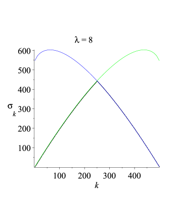
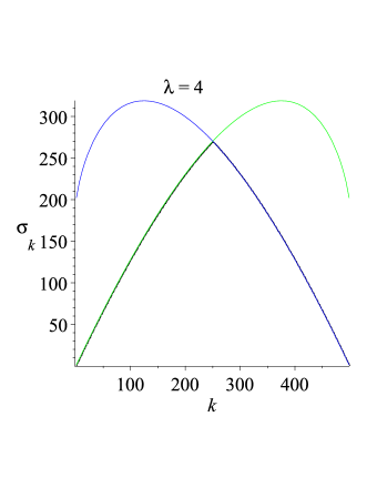
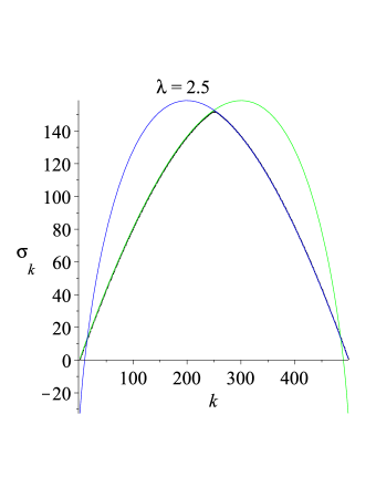
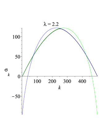
Figure 2: $\sigma_{k}$ as a function of $k$ for $N=500$. The green and blue solid lines are obtained from the first and second terms in equation (22) respectively, while discrete points (black) are computed directly from equation (16) with a discrete density $\rho(\phi)$.

In summary, $\sigma_{k}$ depends on whether $\tfrac{k}{N}$ is greater than or less than $\tfrac{1}{2}$,

$$\sigma_{k}=\left\{\begin{array}[]{ll}-k-(N-k)\ln(1-\tfrac{k}{N})+k\ln\lambda&\tfrac{k}{N}\leq\tfrac{1}{2}~{},~{}\lambda>2\\ -(N-k)+k\ln\tfrac{k}{N}+(N-k)\ln\lambda&\tfrac{k}{N}\geq\tfrac{1}{2}~{},~{}\lambda>2\end{array}\right.$$ (23)

These are accurate to the leading order in large $N$, ${\cal O}(N)$, when $k\sim N$ and we expect that there are corrections of order one, ${\cal O}(N^{0})$. The result has an explicit $k\to N-k$ duality which is obtained by exchanging the saddle points. This exchange of saddle points is a first order phase transition (the first derivative by $\tfrac{k}{N}$ is discontinuous at $\tfrac{k}{N}=\tfrac{1}{2}$).

We recall that for a single box fundamental Wilson loop in the strong coupling phase of the Gross-Witten model [12], $\sigma_{1}=\ln\lambda$. In the top expression in (23), we can clearly identify the contribution from the energies of the $k$ fundamental strings, $k\sigma_{1}=k\ln\lambda$. We can also confirm from the remaining contributions in (23) that the $k$-string tension is indeed always less, that is $\sigma_{k}\leq k\sigma_{1}$, as expected for a stable $k$-string. In fact, for small $\tfrac{k}{N}$,

$$\sigma_{k}=k\sigma_{1}-\frac{k^{2}}{2N}+\ldots~{}.$$ (24)

As in the continuum string tension, the correction is of order $1/N$, rather than $1/N^{2}$.

It is interesting to compare the string tensions in (23) with those in the symmetric representation [19]

$$\sigma_{{\cal S}_{k}}=(N+k)\ln(1+\tfrac{k}{N})+k\ln\lambda-k~{},~{}\lambda<2~{}.$$ (25)

The symmetric string tension is always larger than the tension of $k$ single strings, $\sigma_{{\cal S}_{k}}\geq k\sigma_{1}\geq\sigma_{k}$, even for small $\tfrac{k}{N}$ where $\sigma_{{\cal S}_{k}}=k\sigma_{1}+\frac{k^{2}}{2N}+\ldots$. This is consistent with the idea that representations other than the antisymmetric one should have higher energies. Also, as expected, the symmetric representation tension is not identical to the antisymmetric one, as there are no dynamical gluons to implement screening. In this representation, the strings seem to repel each other.

Now let us consider the weakly coupled, gapped phase with eigenvalue distribution (9). The string tension is obtained by integrating (17) to get the exponent

$$-\int d\phi\rho(\phi)\ln\left(1+\hat{t}e^{i\phi}\right)~{}+~{}\tfrac{k}{N}\ln\hat{t}=$$ (26)

$$-\frac{(\hat{t}+1)\left(\hat{t}+1-\sqrt{(\hat{t}+1)^{2}-2\lambda\hat{t}}\right)}{2\lambda\hat{t}}+\ln\frac{\hat{t}+1-\sqrt{(\hat{t}+1)^{2}-2\lambda\hat{t}}}{\lambda\hat{t}}+\frac{1}{2}+\frac{k}{N}\ln\hat{t}~{},$$

where $\hat{t}$ is adjusted to be an extremum of this expression. Setting the derivative of the above expression by $\hat{t}$ to zero yields an equation that is identical to the result of taking the integral over the eigenvalue density (9) in the saddle-point equation (17),

$$\tfrac{k}{N}-\tfrac{1}{2}=(\hat{t}-1)\frac{\hat{t}+1-\sqrt{(\hat{t}+1)^{2}-2\lambda\hat{t}}}{2\lambda\hat{t}}~{}~{},~{}~{}\lambda\leq 2~{}.$$ (27)

The position of the cut singularity in the square root is determined by the cut singularity of the resolvent in the saddle-point equation (17). The cut is on the unit circle, antipodal to the region where the eigenvalue density has support. The cut crosses the negative real axis at $\hat{t}=-1$. The sign of the square root has been adjusted so that it has the right behavior at $t\sim 0$. As we follow the negative real axis, the sign must flip at $t=-1$ so that the expression has the correct large (negative) $t$ behavior. There are two solutions

$$\hat{t}_{\pm}=\frac{1-\tfrac{\lambda}{4}\left(1-2\tfrac{k}{N}\right)^{2}}{2\left(1-\tfrac{k}{N}\right)}\pm\frac{1-2\tfrac{k}{N}}{2\left(1-\tfrac{k}{N}\right)}\sqrt{\tfrac{\lambda^{2}}{16}\left(1-2\tfrac{k}{N}\right)^{2}+1-\tfrac{\lambda}{2}}~{}.$$ (28)

The argument of the square root in this expression is positive in the domain of parameters of interest. Both roots are non-negative real numbers which can vanish only when $\tfrac{k}{N}=0$ or $\tfrac{k}{N}=1$. They are related by

$$t_{+}t_{-}=\frac{\tfrac{k}{N}}{1-\tfrac{k}{N}}~{}~{},~{}~{}t_{-}\left(\tfrac{k}{N}\right)=\frac{1}{t_{+}\left(1-\tfrac{k}{N}\right)}~{}.$$ (29)

Note that this is similar to the relationship in (20) and (21). For real values of the parameters $\lambda$ and $\tfrac{k}{N}$, the argument of the square root in (28) is always positive, so this square root is unambiguously defined in the entire region of interest. It does have two branches which can both be confirmed to satisfy the saddle-point equation. It’s the smaller root, $t_{-}$, which lives on the first sheet and goes to zero as $\tfrac{k}{N}\rightarrow 0$, that will turn out to be the correct one to use based on the discrete density calculation.

We can substitute $t_{-}$ into (28), taking into account the normalization by adding $\ln{\rm dim}{\cal A}_{k}=\ln(N!/k!(N-k)!)$ to the result, to get the tension

$$\frac{1}{N}\sigma_{k} = -\tfrac{k}{N}\ln\tfrac{k}{N}-(1-\tfrac{k}{N})\ln(1-\tfrac{k}{N})-\frac{2}{\lambda}\left[1-\tfrac{\lambda}{4}-\sqrt{1-\tfrac{\lambda}{2}+\tfrac{\lambda^{2}}{16}(1-2\tfrac{k}{N})^{2}}\right]$$ (30)

$$+ \ln\frac{2}{\lambda}\left[1+\tfrac{\lambda}{4}(1-2\tfrac{k}{N})-\sqrt{1-\tfrac{\lambda}{2}+\tfrac{\lambda^{2}}{16}(1-2\tfrac{k}{N})^{2}}\right]$$

$$+ \frac{k}{N}\ln\frac{1-\tfrac{\lambda}{4}(1-2\tfrac{k}{N})^{2}-(1-2\tfrac{k}{N})\sqrt{1-\tfrac{\lambda}{2}+\tfrac{\lambda^{2}}{16}(1-2\tfrac{k}{N})^{2}}}{2(1-\tfrac{k}{N})}~{}.$$

Similar expression can be obtained starting with the other root, $t_{+}$. Fig. (3) summarizes the results: even though the second sheet saddle point is smaller, it is the first sheet result stated above which agrees with a discrete eigenvalue density computation.

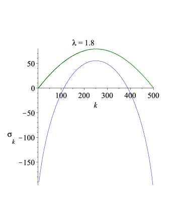
Figure 3: $\sigma_{k}$ as a function of $k$ for $N=500$ in the weakly coupled phase. The green and blue solid lines correspond to equation 30 and a similar expression obtained for the other sheet of the saddle point equation. The green line represents our result for the $k$-string tension in the semi-circle distribution. Discrete points (black) are computed directly from equation (16) using a discrete eigenvalue density.

Though it is not immediately obvious from expression (30), the tension is symmetric under replacement of $\tfrac{k}{N}$ by $1-\tfrac{k}{N}$. This is clearly seen in Fig. 3.

For small $\tfrac{k}{N}$,

$$\sigma_{k}=k~{}\ln\frac{1}{1-\tfrac{\lambda}{4}}~{}-~{}\frac{k^{2}}{N}~{}\frac{\lambda(8-3\lambda)}{2(4-\lambda)^{2}}~{}+~{}{\cal O}\left(\frac{k^{3}}{N^{2}}\right)~{},$$ (31)

where, as expected, the string tension for a $k=1$ string in the weak coupling phase is $\sigma_{1}=\ln\frac{1}{1-\tfrac{\lambda}{4}}$ [12]. As in the strong coupling phase, the interaction term is attractive and is suppressed by one factor of $1/N$. We can also confirm that the interaction is attractive for all values of $0<\tfrac{k}{N}<1$ and for all $0\leq\lambda\leq 2$.

On the other hand, in the weak coupling phase, the symmetric representation string tension can be deduced from the results in Ref. [19]

$$\frac{1}{N}\sigma_{{\cal S}_{k}} = -\tfrac{k}{N}\ln\tfrac{k}{N}+(1+\tfrac{k}{N})\ln(1+\tfrac{k}{N})+\frac{2}{\lambda}\left[1-\tfrac{\lambda}{4}-\sqrt{1-\tfrac{\lambda}{2}+\tfrac{\lambda^{2}}{16}(1+2\tfrac{k}{N})^{2}}\right]$$ (32)

$$- \ln\frac{2}{\lambda}\left[1+\tfrac{\lambda}{4}(1+2\tfrac{k}{N})-\sqrt{1-\tfrac{\lambda}{2}+\tfrac{\lambda^{2}}{16}(1+2\tfrac{k}{N})^{2}}\right]$$

$$+ \frac{k}{N}\ln\frac{-1+\tfrac{\lambda}{4}(1+2\tfrac{k}{N})^{2}+(1+2\tfrac{k}{N})\sqrt{1-\tfrac{\lambda}{2}+\tfrac{\lambda^{2}}{16}(1+2\tfrac{k}{N})^{2}}}{2(1+\tfrac{k}{N})}~{}.$$

By considering the small $\tfrac{k}{N}$ limit, $\sigma_{{\cal S}_{k}}=k\ln\frac{1}{1-\tfrac{\lambda}{4}}~{}+~{}\frac{k^{2}}{N}~{}\frac{\lambda(8-3\lambda)}{2(4-\lambda)^{2}}~{}+~{}{\cal O}\left(\frac{k^{3}}{N^{2}}\right)$, we see that, in the symmetric representation, the interaction is repulsive. It is possible to show that it is is repulsive for all values of $\tfrac{k}{N}>0$ and for all values of $\lambda\leq 2$.

In conclusion, we have found explicit formulae for the $k$-string tension in both the weak and strong coupling phases of 2 dimensional lattice Yang-Mills theory. These formulae differ from the continuum result, which is the quadratic Casimir of the representation. They nevertheless share the property that the interaction between elementary strings is attractive when the quark sources are in the antisymmetric representation and repulsive when they are in the symmetric representation. Furthermore, in the weak coupling phase the $k\to N-k$ duality is realized by a first order phase transition at $k=\tfrac{N}{2}$. An interesting check of the validity of these results is to examine the continuum limit. The weak coupling phase has a good continuum limit as $\lambda\to 0$. In that limit, we should send the lattice spacing to zero, $a\to 0$ while holding the string tension fixed. If we require that the $k=1$ string tension in inverse distance units

$$\sigma_{1}=\frac{1}{a^{2}}\ln\frac{4}{4-\lambda}$$ (33)

remains finite, we must tune the coupling constant as $\lambda=4-4e^{-\sigma_{1}a^{2}}$. Using this in the $k$-string tension (30), we obtain

$$\sigma_{k}=k\left(1-\tfrac{k}{N}\right)\sigma_{1}~{}+~{}\frac{k^{2}}{3N}\left(\left(1-\tfrac{k}{N}\right)a^{2}\sigma_{1}\right)^{2}\sigma_{1}~{}+~{}{\cal O}(a^{6})~{}.$$ (34)

Similarly, for the symmetric representation in (32), the continuum limit yields

$$\sigma_{{\cal S}_{k}}=k\left(1+\tfrac{k}{N}\right)\sigma_{1}~{}-~{}\frac{k^{2}}{3N}\left(\left(1+\tfrac{k}{N}\right)a^{2}\sigma_{1}\right)^{2}\sigma_{1}~{}+~{}{\cal O}(a^{6})~{}.$$ (35)

The leading terms are in agreement with the Casimir scaling (3) which is known to be the exact behavior of continuum 2-dimensional Yang-Mills theory.

The authors acknowledge hospitality of the Galileo Galilei Institute, Khavli Institute for Theoretical Physics, Santa Barbara, the Aspen Center for Physics and the Perimeter Institute. This work is supported in part by NSERC of Canada.

References

- [1] M. J. Strassler, “Messages for QCD from the superworld,” Prog. Theor. Phys. Suppl. 131 (1998) 439 [arXiv:hep-lat/9803009].
- [2] M. J. Strassler, “QCD, supersymmetric QCD, lattice QCD and string theory: Synthesis on the horizon?,” Nucl. Phys. Proc. Suppl. 73, 120 (1999) [arXiv:hep-lat/9810059].
- [3] L. Del Debbio, H. Panagopoulos and E. Vicari, “Confining strings in representations with common n-ality,” JHEP 0309, 034 (2003) [arXiv:hep-lat/0308012].
- [4] L. Del Debbio, H. Panagopoulos, P. Rossi and E. Vicari, “Spectrum of confining strings in SU(N) gauge theories,” JHEP 0201, 009 (2002) [arXiv:hep-th/0111090].
- [5] J. Greensite and S. Olejnik, “K-string tensions and center vortices at large N,” JHEP 0209, 039 (2002) [arXiv:hep-lat/0209088].
- [6] A. Armoni and M. Shifman, “On k-string tensions and domain walls in N = 1 gluodynamics,” Nucl. Phys. B 664, 233 (2003) [arXiv:hep-th/0304127].
- [7] A. Armoni and M. Shifman, “Remarks on stable and quasi-stable k-strings at large N,” Nucl. Phys. B 671, 67 (2003) [arXiv:hep-th/0307020].
- [8] C. P. Korthals Altes and H. B. Meyer, “Hot QCD, k-strings and the adjoint monopole gas model,” arXiv:hep-ph/0509018.
- [9] P. Orland, “String tensions and representations in anisotropic (2+1)-dimensional weakly-coupled Yang-Mills theory,” Phys. Rev. D 75, 025001 (2007) [arXiv:hep-th/0608067].
- [10] B. Bringoltz and M. Teper, “Closed k-strings in SU(N) gauge theories : 2+1 dimensions,” Phys. Lett. B 663, 429 (2008) [arXiv:0802.1490 [hep-lat]].
- [11] M. R. Douglas and S. H. Shenker, “Dynamics of SU(N) supersymmetric gauge theory,” Nucl. Phys. B 447, 271 (1995) [arXiv:hep-th/9503163].
- [12] D. J. Gross and E. Witten, “Possible Third Order Phase Transition In The Large N Lattice Gauge Theory,” Phys. Rev. D 21 (1980) 446.
- [13] S. B. Khokhlachev and Yu. M. Makeenko, “Phase Transition Over Gauge Group Center And Quark Confinement In QCD,” Phys. Lett. B 101, 403 (1981).
- [14] A. Dumitru, Y. Hatta, J. Lenaghan, K. Orginos and R. D. Pisarski, “Deconfining phase transition as a matrix model of renormalized Polyakov loops,” Phys. Rev. D 70, 034511 (2004) [arXiv:hep-th/0311223].
- [15] R. D. Pisarski, “Gross-Witten Point And Deconfinement,” Int. J. Mod. Phys. A 20, 4469 (2005).
- [16] A. Hanany, M. J. Strassler and A. Zaffaroni, “Confinement and strings in MQCD,” Nucl. Phys. B 513, 87 (1998) [arXiv:hep-th/9707244].
- [17] C. P. Herzog and I. R. Klebanov, “On string tensions in supersymmetric SU(M) gauge theory,” Phys. Lett. B 526, 388 (2002) [arXiv:hep-th/0111078].
- [18] Shuhang Yang, “Large Gauge Theory and -Strings”, UBC MSc Thesis, 2010.
- [19] G. Grignani, J. L. Karczmarek and G. W. Semenoff, “Hot Giant Loop Holography,” Phys. Rev. D 82, 027901 (2010) [arXiv:0904.3750 [hep-th]].
- [20] S. A. Hartnoll and S. P. Kumar, “Higher rank Wilson loops from a matrix model,” JHEP 0608, 026 (2006) [arXiv:hep-th/0605027].