Tunnelling between edge states of a 2D topological insulator and a Fermi liquid lead through a quantum dot

Abstract

In this paper we study a non-equilibrium resonant tunnelling problem where a non-interacting quantum dot is connected to two leads, one being the edge of an interacting 2-D topological insulator (Luttinger liquid) and the other being a usual Fermi liquid. We show that the current passing through the system can be expressed in terms of a non-equilibrium local single-particle Green’s function of the Luttinger liquid lead which can be analysed using standard bosonization-Renormalization Group (RG) technique. In particular, some exact results can be extracted in the small bias limit with repulsive electron-electron interaction. A simple formula which captures the qualitative feature of the I-V relation over whole temperature and voltage bias range is being proposed and studied.

The discovery of topological insulatorstopological insulator1 ; topological insulator2 has generated much interests and activities in the condensed matter physics community. In the case of 2-D topological insulators (Quantum Spin-Hall systems), helical edge states respecting time-reversal symmetrySCZhang exist and provide an example of interacting Luttinger liquid which can be studied experimentally up to room temperature. The transport properties of interacting one-dimensional systems have been studied extensively in the literatureKane&Fisher ; Furusaki&Nagaosa ; Fabrizio&Gogolin , especially after the discovery of edge states in fractional quantum hall (FQH) liquids Res-Tun in FQH (chiral Luttinger liquids). For example, the problem of non-interacting quantum dot connected to leads of FQH edge states was studied by Chamon and WenChamon & Wen , and later by Furusaki Furusaki at temperatures higher than the tunnelling strength.

The emergence of topological insulator makes these 1-D theoretical models realizable. In this paper we study a simple model of a non-interacting quantum dot connected to two leads, one being the edge of 2-D topological insulator with electron-electron interaction, the other being a normal Fermi liquid lead (Fig.1). We show here that the non-linear I-V relation of the system can be expressed in terms of a non-equilibrium local single-particle Green’s function of the topological insulator lead which can be analyzed in the limit of small voltage bias and low temperature using a conventional renormalization-group (RG) approach. A few exact results are extracted from the RG analysis and a simple formula which captures the qualitative feature of the I-V relation over whole temperature and voltage bias range is being proposed and studied in this paper.

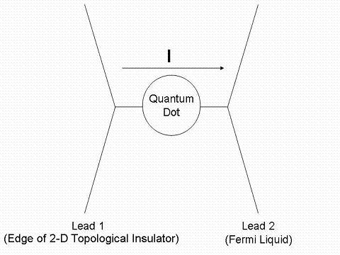
Figure 1: The configuration

We start with the model Hamiltonian $H=H_{01}+H_{02}+H_{0d}+H_{T}$, where

$$H_{01} = -iv_{F}\int dx(\hat{\psi}_{1R,\uparrow}^{+}(x)\partial_{x}\hat{\psi}_{1R,\uparrow}(x)$$ (1a)

$$-\hat{\psi}_{1L,\downarrow}^{+}(x)\partial_{x}\hat{\psi}_{1L,\downarrow}(x))$$

$$+\frac{g}{2}\int dx(\hat{\psi}_{1R,\uparrow}^{+}(x)\hat{\psi}_{1R,\uparrow}(x)$$

$$+\hat{\psi}_{1L,\downarrow}^{+}(x)\hat{\psi}_{1L,\downarrow}(x))^{2}$$

and

$$H_{02}=\sum_{k,\sigma}\varepsilon_{2k}\hat{c}_{2k,\sigma}^{+}\hat{c}_{2k,\sigma}$$ (1b)

are terms in the Hamiltonian describing the edge of a 2-D topological insulator ($$H_{01} H_{02}$$) and the Fermi liquid lead (), respectively.

$$H_{0d}=\varepsilon_{0}\sum_{\sigma}\hat{d}_{\sigma}^{+}\hat{d}_{\sigma}$$ (1c)

is the Hamiltonian describing the quantum dot and

$$H_{T} = T_{1}\{\hat{\psi}_{1R,\uparrow}^{+}(0)\hat{d}_{\uparrow}+\hat{\psi}_{1L,\downarrow}^{+}(0)\hat{d}_{\downarrow}+h.c\}$$ (1d)

$$+T_{2}\{\hat{\psi}_{2,\uparrow}^{+}(0)\hat{d}_{\uparrow}+\hat{\psi}_{2,\downarrow}^{+}(0)\hat{d}_{\downarrow}+h.c\}$$

describes electron tunnelling between the dot and the leads. We note that since the propagation and spin directions of electrons in the topological insulator lead are tied together (helical edge), we can forget its spin suffix and the helical edges states of topological insulator behave like a spinless Luttinger Liquid Luttinger Liquid ; vic .

$H_{01}$ can be transformed to a free boson system by standard bosonization technique Giamarchi where the fermion correlation function $g_{1}(t,t^{\prime})\equiv-i\left\langle T_{C}\hat{\psi}_{1,\sigma}(0,t)\hat{\psi}^{+}_{1,\sigma}(0,t^{\prime})\right\rangle_{H_{01}}$ can be computed straightforwardlyMy thesis . In bosonization theory a Luttinger liquid is usually characterized by the interaction strength parameter $K\equiv(1+\frac{g}{\pi v_{F}})^{-1/2}$; here we further define $\vartheta\equiv\frac{1}{2}(K+\frac{1}{K}-2)$ which is a parameter we shall use frequently in the following.

The DC current $I$ flowing from lead 1 to 2 in the above system can be expressed asMeir&Wingreen&Jauho

$$I = -I_{2}=e\sum_{\sigma}\left\langle\frac{dN_{2\sigma}}{dt}\right\rangle$$ (2)

$$= -ieT_{2}\sum_{\sigma}\left\langle\hat{\psi}_{2,\sigma}^{+}(0,t)\hat{d}_{\sigma}(t)-\hat{d}^{+}_{\sigma}(t)\hat{\psi}_{2,\sigma}(0,t)\right\rangle$$

where $I_{2}$ is the current flowing from lead 2 to the quantum dot. Since lead 2 is non-interacting, we can eliminate the lead-2 electron operators through their equation of motion. Following Ref.Meir&Wingreen&Jauho we obtain after some straightforward algebra

$$I = -e|T_{2}|^{2}\sum_{\sigma}\int d\varepsilon\rho_{2}(\varepsilon)[2f(\varepsilon-\mu_{2})\mathrm{Im}\{G_{dd,\sigma}^{R}(\varepsilon)\}$$ (3)

$$+\mathrm{Im}\{G_{dd,\sigma}^{<}(\varepsilon)\}]$$

where $G_{dd,\sigma}^{R}(\varepsilon)$ and $G_{dd,\sigma}^{<}(\varepsilon)$ are the Fourier Transform of the “retarded” and “less” components of the on-site (Keldysh) Green’s function of the quantum dot, $G_{dd,\sigma}(t,t^{\prime})\equiv-i\left\langle T_{C}\hat{d}_{\sigma}(t)\hat{d}^{+}_{\sigma}(t^{\prime})\right\rangle$, where $t$ and $t^{\prime}$ are time-ordered along a closed time contour from $t=-\infty$ to $t=\infty$ and then back to $t=-\infty$. $\rho_{2}(\varepsilon)$ and $\mu_{2}$ are the density of states (which will be taken to be a constant later) and chemical potential of lead 2, respectively. $f(\varepsilon)$ is the Fermi-distribution function. Notice that the current is expressed solely in terms of a (non-equilibrium) local single-particle Green’s function of the system. This result is possible because lead 2 is non-interacting.

To calculate $G_{dd,\sigma}$ we follow the Keldysh path integral formalism Kamenev . The action of the system is Vurkevich

$$S = \int_{C}dt[\int dx\sum_{\sigma}\{\bar{\psi}_{1,\sigma}(x,t)i(\partial_{t}+\sigma v_{F}\partial_{x})\psi_{1,\sigma}(x,t)\}$$

$$-\frac{g}{2}\int dx(\sum_{\sigma}\bar{\psi}_{1,\sigma}(x,t)\psi_{1,\sigma}(x,t))^{2}$$

$$+\sum_{k,\sigma}\bar{c}_{2k,\sigma}(t)(i\partial_{t}-\varepsilon_{2k})c_{2k,\sigma}(t)$$

$$+\sum_{\sigma}\{T_{1}\bar{\psi}_{1,\sigma}(0,t)d_{\sigma}(t)+T_{2}\bar{\psi}_{2,\sigma}(0,t)d_{\sigma}(t)+c.c\}$$

$$+\sum_{\sigma}\bar{d}_{\sigma}(t)(i\partial_{t}-\varepsilon_{0})d_{\sigma}(t)+\sum_{\sigma}\{\bar{\xi}_{\sigma}(t)d_{\sigma}(t)+c.c\}]$$

where $\sigma=\pm 1$ and we have suppressed the propagation direction indices of the helical edge states for brevity. $\{\xi_{\sigma},\bar{\xi}_{\sigma}\}$ are external source fields introduced to generate $G_{dd,\sigma}(t,t^{\prime})$. Integrating out the fermionic fields $\{c_{2k,\sigma},\bar{c}_{2k,\sigma}\}$ and $\{d_{\sigma},\bar{d}_{\sigma}\}$ we obtain

$$S_{eff} = \int_{C}dt[\int dx\sum_{\sigma}\{\bar{\psi}_{1,\sigma}(x,t)i(\partial_{t}+\sigma v_{F}\partial_{x})\psi_{1,\sigma}(x,t)\}$$ (5)

$$-\frac{g}{2}\int dx(\sum_{\sigma}\bar{\psi}_{1,\sigma}(x,t)\psi_{1,\sigma}(x,t))^{2}]$$

$$-\sum_{\sigma}\int_{C}dt_{1}dt_{2}[\bar{\xi}_{\sigma}(t_{1})+T_{1}\bar{\psi}_{1,\sigma}(0,t_{1})]g_{D\sigma}(t_{1},t_{2})\times$$

$$[\xi_{\sigma}(t_{2})+T_{1}^{*}\psi_{1,\sigma}(0,t_{2})]$$

which is an effective action for lead-1 electrons only. $g_{D\sigma}(t,t^{\prime})$ is the Green’s function of the quantum dot evaluated under the “dot+lead 2” action with

$$g^{R/A}_{D\sigma}(\omega) = \frac{1}{\omega-\varepsilon_{0}\pm i\Gamma_{2}}$$ (6)

$$g^{<}_{D\sigma}(\omega) = \frac{2i\Gamma_{2}f(\omega-\mu_{2})}{(\omega-\varepsilon_{0})^{2}+\Gamma_{2}^{2}},$$

where $\Gamma_{1(2)}=\pi\rho_{1(2)}|T_{1(2)}|^{2}$ is the tunnelling width from the dot to lead $1(2)$. $G_{dd,\sigma}(t,t^{\prime})$ can be obtained by taking functional derivatives of the generating functional with respect to the $\{\xi_{\sigma},\bar{\xi_{\sigma}}\}$ fields; we obtain

$$G_{dd,\sigma}(t,t^{\prime}) = g_{D\sigma}(t,t^{\prime})+|T_{1}|^{2}\int_{C}dt_{1}dt_{2}g_{D\sigma}(t,t_{1})\times$$ (7)

$$g_{1\sigma eff}(t_{1},t_{2})g_{D\sigma}(t_{2},t^{\prime})$$

where

$$g_{1\sigma eff}(t,t^{\prime})\equiv-i\left\langle T_{C}\hat{\psi}_{1,\sigma}(0,t)\hat{\psi}^{+}_{1,\sigma}(0,t^{\prime})\right\rangle_{eff}$$

is the Green’s function of lead-1 electrons evaluated at $x=0$ according to the effective action (5) in the absence of the external source terms. Different Keldysh components of $G_{dd,\sigma}$ can be extracted from (7) using Langreth’s sum rules Langreth sum rule . Combining Eqs. (6) and (7), we obtain for the tunnelling current (3),

$$I = -e|T_{1}|^{2}|T_{2}|^{2}\sum_{\sigma}\int d\omega\rho_{2}\frac{1}{(\omega-\varepsilon_{0})^{2}+\Gamma_{2}^{2}}\times$$ (8)

$$\{\mathrm{Im}g_{1\sigma eff}^{<}(\omega)+2f(\omega-\mu_{2})\mathrm{Im}g_{1\sigma eff}^{R}(\omega)\}.$$

where the only unknown is the effective green’s function $g_{1\sigma eff}(t,t^{\prime})$.

To evaluate $g_{1\sigma eff}(t,t^{\prime})$ we express it in the form of a standard Dyson’s equation

$$g_{1\sigma eff}(t,t^{\prime}) = g_{1\sigma}(t,t^{\prime})+\int_{C}dt_{1}dt_{2}g_{1\sigma}(t,t_{1})\Sigma_{\sigma,T}(t_{1},t_{2})$$ (9)

$$\times g_{1\sigma eff}(t_{2},t^{\prime})$$

where $g_{1\sigma}(t,t^{\prime})$ is the Green’s function of lead-1 electrons at $x=0$ evaluated at $T_{1}=0$, and is the standard $x=0$ Green’s function of spinless Luttinger liquid with interaction strength $K$Giamarchi . The self-energy term in (9) represents correction coming from the tunnelling term (last term in Eq.(5)). The tunnelling current (8) can be expressed in terms of the Fourier-transformed self-energy $\Sigma_{\sigma,T}(\omega)$ as

$$I = -e|T_{1}|^{2}|T_{2}|^{2}\sum_{\sigma}\int d\omega\rho_{2}\times$$ (10)

$$\mathrm{Im}\{\frac{2(f(\omega-\mu_{2})-f(\omega-\mu_{1}))g_{1\sigma}^{R}(\omega)-\left|g_{1\sigma}^{R}(\omega)\right|^{2}(\Sigma_{\sigma,T}^{<}(\omega)+2f(\omega-\mu_{2})\Sigma_{\sigma,T}^{R}(\omega))}{\left|1-g_{1\sigma}^{R}(\omega)\Sigma_{\sigma,T}^{R}(\omega)\right|^{2}((\omega-\varepsilon_{0})^{2}+\Gamma_{2}^{2})}\}.$$

We observe that the tunnelling current is completely determined by the self-energy function $\Sigma_{\sigma,T}(\omega)$. In the absence of electron-electron interaction $\Sigma_{\sigma,T}(\omega)=\Sigma^{(0)}_{\sigma,T}(\omega)=|T_{1}|^{2}g_{D\sigma}(\omega)$ and our main job here is to understand how $\Sigma^{(0)}_{\sigma,T}(\omega)$ is renormalized by the electron-electron interaction.

In the following we shall study $\Sigma_{\sigma,T}$ in the small bias, low temperature limit $T,|\mu_{1}-\mu_{2}|<<\Gamma_{1(2)}$ using a standard bosonization-RG analysisKane&Fisher . In this limit we may keep only the long-time behavior of $g_{D\sigma}(t)$ in Eq. (5) and forget about the more complicated intermediate time behaviors, i.e. we approximate

$$g_{D\sigma}^{R(A)}(t) = e^{i\varepsilon_{0}t-\Gamma_{2}|t|}|_{t\rightarrow\infty}\rightarrow 0,$$ (11)

$$g_{D\sigma}^{<}(t) \sim 2i{\Gamma_{2}\over\varepsilon_{0}^{2}+\Gamma_{2}^{2}}{e^{i\mu_{2}t}\over t}.$$

To proceed further we compare the present problem with the problem of directly tunnelling between a Luttinger liquid and a Fermi liquid through a simple tunnelling junction barrier $t$. The Fermi liquid fields can be integrated out as what we have done to derive Eq. (5). The only difference in the direct tunnelling problem is that $g_{D\sigma}(t)$ in Eq. (5) is replaced by $g_{0\sigma}^{R(A)}(t)\sim\mp i\pi N(0)\delta(t)$ and $g_{0\sigma}^{<}(t)\sim 2iN(0)e^{i\mu_{2}t}/t$ where $N(0)$ is the density of states on the Fermi surface. Comparing with Eq. (11) We see that the resonant tunnelling problem reduces to the direct tunnelling problem in this limit if we replace the dimensionless tunnelling parameter $tN(0)\rightarrow T_{1}\sqrt{\Gamma_{2}\over\varepsilon_{0}^{2}+\Gamma_{2}^{2}}$ and the scaling behavior of the self-energy in the present problem can be inferred from the corresponding direct tunnelling problem which has been analyzed using well-developed bosonization-RG technique. We obtain immediately

$$T_{1}(E)\sim(E/E_{F})^{1-K_{eff}},$$

in this approximation, where $K_{eff}=2K/(1+K)$Furusaki . In particular for repulsive interaction ($K<1$), $T_{1}(E\rightarrow 0)\rightarrow 0$ and the self-energy scales to zero in the infrared regime, which makes perturbative RG applicable. In this case it is sufficient to approximate $\Sigma_{\sigma,T}\sim\Sigma^{(0)}_{\sigma,T}$ with $T_{1}\rightarrow T_{1}(E)$. Physically, the vanishing of self-energy is an alternative way to express the well known result that the tunnelling between the Luttinger liquid lead and the Fermi liquid lead vanishes in the infrared limitKane&Fisher ; Furusaki . We emphasize here that the renormalization of $T_{1}$ is restricted only to the self-energy term and does not appear in other places in the current expression. With this approximation we obtain

$$I\sim-2e{|T_{1}|^{2}\Gamma_{2}\over\pi}\sum_{\sigma}\int d\omega(f(\omega-\mu_{2})-f(\omega-\mu_{1}))\frac{Im[g_{1\sigma}^{R}(\omega)]}{\left|\omega-\varepsilon_{0}+i\Gamma_{2}-|T_{1}(E)|^{2}g_{1\sigma}^{R}(\omega)\right|^{2}}.$$ (12)

where $E=max\{T,|\omega-\mu_{1}|\}$. Eq. (12) is expected to be reliable in both the low temperature, small bias limit $(T,|\mu_{1}-\mu_{2}|)<<\Gamma_{1(2)}$ and in the high temperature, large bias limit $(T,|\mu_{1}-\mu_{2}|)\sim E_{F}$ where $T_{1}(E)\rightarrow T_{1}$ and the renormalization of $T_{1}$ becomes unimportant. We shall analyze the current using this approximate formula in the following.

To study the tunnelling characteristics, we define $eV\equiv\mu_{2}-\mu_{1}$ and $\varepsilon\equiv\varepsilon_{0}-\mu_{1}$ and look at the differential conductance $\frac{dI}{dV}$ as function of $V$ at different temperature regimes. Using the result that $g_{1\sigma}^{R}(\omega)\sim E^{\theta}$ and approximating the Lorentzian function by a $\delta$-function, we find that at very high-temperature regime ($T\gg\Gamma_{1,2},\varepsilon_{0}$), $T_{1}(E)\rightarrow T_{1}$ and $\frac{dI}{dV}$ scales with temperature as $T^{\vartheta-1}$, in agreement with Furusaki’s result Furusaki . On the other hand, the low temperature regime $T\ll\Gamma_{1,2}$ can be sub-divided into two regions: when $eV\ll T$, the linear differential conductance scales as $T^{\theta}(1+aT^{\gamma})$, where $\gamma=\mathrm{min}\{1,\vartheta+2(1-K_{eff})\}$ and $a$ is a temperature-independent constant; but when $eV\gg T\rightarrow 0$, the current-voltage relation becomes non-linear and ${dI\over dV}$ becomes $V-$dependent(see discussion below) at small $V$. The different scaling behaviors are summarized in Fig.2.

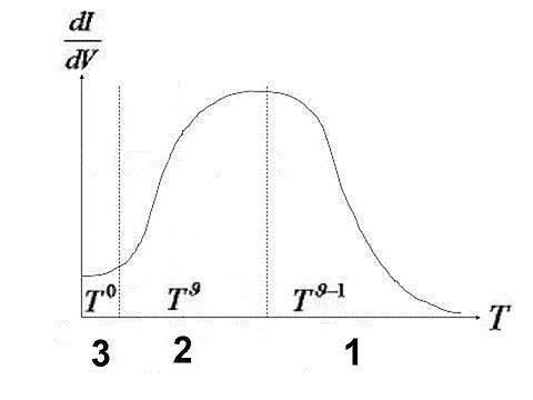
Figure 2: The leading-order temperature dependence of differential conductance in different regimes. Regime 1: $T>>\Gamma_{1,2}$; Regime 2: $|eV|<<T<<\Gamma_{1,2}$; Regime 3: $T<<|eV|$.

Next we consider (non-linear) differential conductance at zero temperature. First, we observe that in the off-resonance region ($|eV|,\Gamma_{1,2}\ll\varepsilon$), the differential conductance goes as $|V|^{\vartheta}(1+a^{\prime}|V|^{\gamma})$, where $a^{\prime}$ (different from $a$) is a temperature-independent constant. The first term ($|V|^{\theta}$) is in agreement with previous resultChamon & Wen and the second term $|V|^{\theta+\gamma}$ is the leading correction coming from scaling of $T_{1}$. Our RG amalysis suggests that the leading order ($|V|^{\theta}$ and $T^{\theta}$) scalings are exact as long as $g_{1\sigma}^{R}(\omega)\Sigma_{\sigma,T}^{R}(\omega)|_{\omega\rightarrow 0}\rightarrow 0$ which is the case for repulsive electron-electron interaction and is independent of the detailed structure of $\Sigma_{\sigma,T}^{R}(\omega)$. The self-energy gives rise only to higher-order corrections to $V/T$ scalings at low temperature and small voltage bias.

We also observe a resonance peak of differential conductance located around $eV\sim\varepsilon$ and the differential conductance at $V=0$ is always zero as long as lead 1 is interacting. This is a character of Luttinger liquids which is very different for non-interacting electrons ($K=1$), where $\frac{dI}{dV}|_{V\rightarrow 0}$ approaches a constant. Finally, when $V$ is far away from the resonant point, the differential conductance falls as $|V|^{\vartheta-2\times\mathrm{max}\{1,\vartheta+2(1-K_{eff})\}}$.

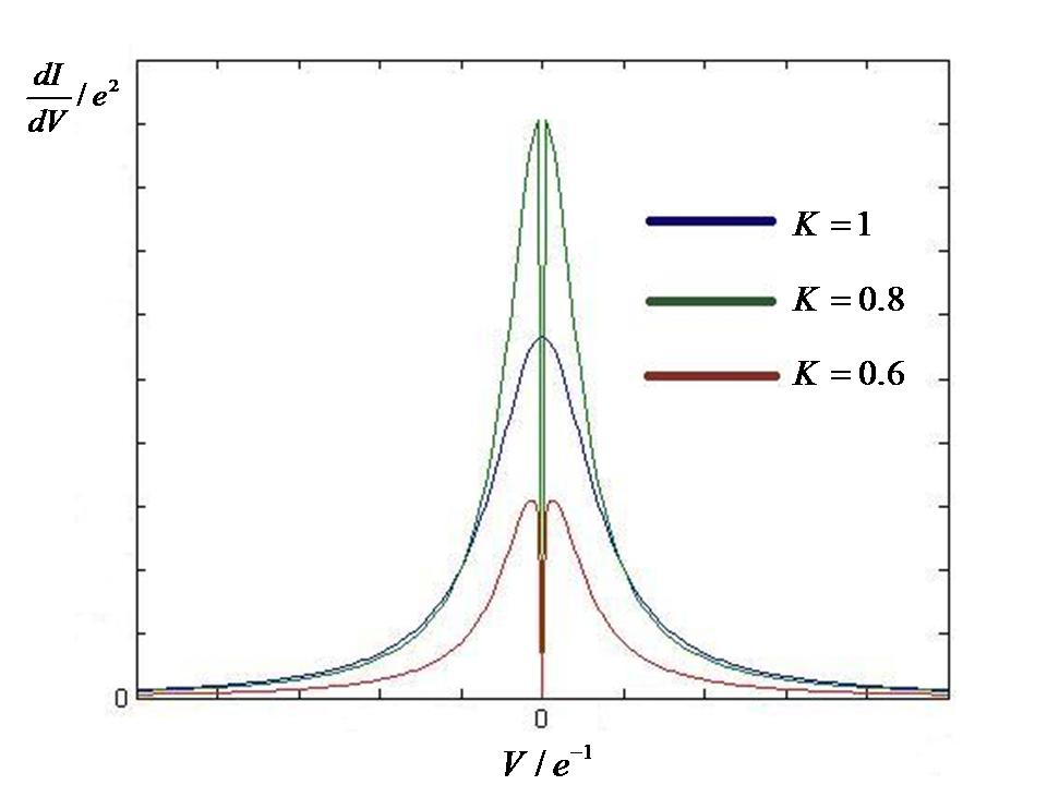
Figure 3: (color online) Differential conductance at zero temperature with $\varepsilon=0$

To conclude, we have extended Meir-Wingreen’s current formula to the case with one interacting lead in this paper, and have used it to calculate the tunnelling current from the edge of a 2D topological insulator through a quantum dot to a normal Fermi liquid lead. The formulation allows us to construct a current expression in terms of the self-energy of a local Green’s function. The differential conductance in different temperature regimes is analyzed using perturbative RG in this paper, which is believed to be reliable when both temperature and voltage bias are much smaller than $\Gamma_{1(2)}$ and if the electron-electron interaction in lead 1 is repulsive. Based on the RG result, an approximate formula for the current qualitatively valid over whole temperature/volatge range is proposed. The formula reproduces results of earlier works at high temperature and produces exact results at low temperature for repulsive electron-electron interaction and small bias. For attractive interaction the scaling breaks down at low enough energy $E$ suggesting that qualitatively new $dI/dV$ behavior is expected at low energy. Our approach offers a new theoretical tool of analysing (non-equilibrium) DC transports which can be extended to other systems with both Luttinger and Fermi liquid leads.

We thank K. T. Law, Zhengxin Liu and C. Chan for useful discussions. This work is supported by HKRGC grant HKUST3/CRF/09.

References

(1) C. L. Kane and E. J. Male, Science,
314, 1692 (2006).
(2) C. L. Kane, Nature, 4,
348 (2008).
(3) C. Wu, B. A. Bernevig and S. C. Zhang, Phys. Rev. Lett. 96, 106401 (2006).
(4) C. L. Kane and M. P. A. Fisher, Phys, Rev. B 46, 15233 (1992).
(5) A. Furusaki and N. Nagaosa, Phys. Rev. B 47, 3827 (1993).
(6) M. Fabrizio and A.O. Gogolin, Phys. Rev. B 50, 17732 (1994).
(7) J. A. Simmons, H. P. Wei, L. W. Engel, D.
C. Tsui and M. Shayegan, Phys. Rev. Lett. 63, 1731 (1989).
(8) C. de C. Chamon and X. G. Wen, Phys. Rev.
Lett. 70, 2605 (1993).
(9) A. Furusaki, Phys. Rev. B 57, 7141 (1998).
(10) J. M. Luttinger, J. Math. Phys. N. Y.
4, 1154 (1963).
(11) K.T. Law, C.Y. Seng, P.A. Lee and T.K. Ng, Phys. Rev. B81, 041305 (2010)
(12) A. Kamenev and A. Levchenko, Adv. Phy. 58,
197 (2009).
(13) See, e.g., T. Giamarchi, Quantum Physics
in One Dimension (Oxford University Press, Cambridge, 1998).
(14) C. Y. Seng, Mphil Thesis, The Hong Kong University of Science and
Technology (2010).
(15) A. P. Jauho, N. S. Wingreen and Y.
Meir, Phys. Rev. B 50, 5528 (1994).
(16) I. V. Lerner and I. V. Vurkevich, in
Nanophysics: Coherence and Transport, edited by H.
Bouchiat, Y. Gefen, S. Gueron, G. Montambaux and J. Dalibard
(Elsevier, New York, 2005)
(17) D. C. Langreth, in Linear and
Nonlinear Electron Transport in Solids, Vol.17 of Nato
Advanced Study Institute, Series B: Physics, edited by J. T.
Devreese and V. E. Van Doren (Plenum, New York, 1976).
(18) X. G. Wen, Quantum Field Theory of Many-Body
Systems (Oxford University Press, 2004).