Adaptive hierarchic transformations for dynamically p𝑝p-enriched slope-limiting over discontinuous Galerkin systems of generalized equations

C. Michoski\htmladdnormallink\textproto\AAsadehttps://webspace.utexas.edu/michoski/Michoski.html ,  C. Mirabito,  C. Dawson,
Institute for Computational Engineering and Sciences (ICES), Computational Hydraulics Group (CHG)
University of Texas at Austin, Austin, TX, 78712

E. J. Kubatko,
Department of Civil and Environmental Enineering and Geodetic Science
The Ohio State University, Columbus, OH, 43210

D. Wirasaet,  J. J. Westerink
Computational Hydraulics Laboratory, Department of Civil Engineering and Geological Sciences
University of Notre Dame, Notre Dame, IN, 46556
Abstract

We study a family of generalized slope limiters in two dimensions for Runge-Kutta discontinuous Galerkin (RKDG) solutions of advection–diffusion systems. We analyze the numerical behavior of these limiters applied to a pair of model problems, comparing the error of the approximate solutions, and discuss each limiter’s advantages and disadvantages. We then introduce a series of coupled p𝑝p-enrichment schemes that may be used as standalone dynamic p𝑝p-enrichment strategies, or may be augmented via any in the family of variable-in-p𝑝p slope limiters presented.

Keywords: Discontinuous Galerkin, finite elements, RKDG, strong stability preserving (SSP), total variation diminishing (TVD), adaptive slope limiting, shock capturing, dynamic p𝑝p-adaptivity, dynamic p𝑝p-enrichment, error analysis, advective transport, hyperbolic PDE.

00footnotetext: \htmladdnormallink\textproto\AAsadehttps://webspace.utexas.edu/michoski/Michoski.htmlCorresponding author, michoski@ices.utexas.edu

1 §​1§1\S 1 Introduction

Generally when solving advection-diffusion equations — which are not strictly diffusion dominated — by way of, for example, finite element or finite volume techniques, one observes the presence of spurious oscillations in the solution space often brought about by the existence of shocks in the space of approximate solutions as well as from the presence of sharp and/or discontinuous profiles in the physical domain itself. Such ill-behaved approximate solutions have led to the development of numerous methods designed with the intent to consistently stabilize and “limit” the solution in order to deal with these oscillations, as they are seen to arise quite frequently in common scientific applications. For example, slope limiters are known to be of central importance in storm surge modeling [8, 32] in order to obtain, for example, well-behaved solutions in the presence of complicated free–boundary conditions along adapting shorelines. Limiting regimes are also of substantial importance in quantum hydrodynamic systems [29, 4] and surface wave models [26] where they are used to reduce the oscillations caused by mathematical dispersion terms (i.e. nonlinear third order spatial derivative terms) that pervade, for example, tunneling solutions. In fact, slope limiters are of fundamental importance in most applications in standard fluid dynamics, being employed commonly in compressible Navier–Stokes [31], Eulers[42], and magnetofluid [39, 17] applications, not to mention the important role limiters play in the study of radiative transfer [15] and kinetic theory [18]; just to note a handful.

From a numerical perspective, it is clear that one should desire that even shock dominated solutions, like both their smooth and non-limited counterparts, converge in p𝑝p as p↗pmax↗𝑝subscript𝑝p\nearrow p_{\max}. However, such convergence is fundamentally coupled to the behavior of the error accumulation with respect to one’s chosen slope limiting methodology, which, it turns out, must operate over a larger number of degrees of freedom, respectively, as p𝑝p increases. For example, in a hierarchical basis (as shown explicitly below) the degrees of freedom grow nonlinearly as a function of p𝑝p and each degree of freedom ends up carrying information of potentially pathological (or undesirable) overshoots and undershoots which have developed over the native (or non-limited) solution space. It turns out that this complication introduces a substantial technical difficulty in practice, which many papers on numerical shock capturing [16, 14, 25, 28, 1, 27, 6, 7, 12] tend to avoid addressing directly. Most noteworthy is the observation that slopelimiters tend to limit the coefficients in their chosen basis independently of each other, in the sense that each component is adjusted based on information about the surrounding solution on a relatively local submanifold of the total domain. It then follows directly that the application of the limiter grows nonlinearly in each timestep as a function of p𝑝p. Since a limiter de jure introduces error into the FEM solution space each time it operates on the FEM solution, more applications of it (iteratively) to the solution space should, as a general rule, lead to greater error accumulation assuming the first application always introduces approximately the same amount of error. In fact, this is what we observe in each of our limiters de facto. However, we offer an alternative approach to this problem below which is both highly efficient and consistent with the more general setting of h​pℎ𝑝hp-adaptivity.

It perhaps comes as no surprise that the same type of complications do not arise with respect to the mesh size hℎh. That is, the convergence in hℎh as h↘hmin↘ℎsubscriptℎh\searrow h_{\min} tends to arise as a natural consequence of the usual hℎh convergence, where convergence seems essentially guaranteed in most reasonable limiting regimes, while the order of convergence most certainly is not [27]. This issue raises another subtle technical difficulty which we will not address directly in this paper, though we will mention its importance in the proper context.

Another important technicality pertaining to computational efficiency arises with respect to the well-known Courant-Friedrichs-Lewy (CFL) condition. In this setting the temporal discretization is (partially) bounded from above by the spatial discretization. That is, in order to reach a higher order accuracy at a fixed value of hℎh one must project onto a higher order polynomial basis in p𝑝p, thus reducing the admissible timestep Δ​tΔ𝑡\Delta t of the scheme — which obeys an inverse relation by virtue of the CFL condition: Δ​t∝1/pproportional-toΔ𝑡1𝑝\Delta t\propto 1/p as discussed in [38].

Since this p𝑝p-dependence on the solution accuracy runs counter to the CFL restriction in a practical computational sense, substantial effort has been invested in developing “smart schemes” which in some way are able to “sense” the appropriate place (e.g. đ’™âˆˆÎ©đ’™Î©\boldsymbol{x}\in\Omega) within the solution domain to enrich the polynomial order p𝑝p, while keeping other areas either unaffected or adaptively de-enriching areas of “less importance.” The ultimate goal of these schemes is to attempt to substantially improve the computational efficiency of the numerical scheme without ceding notable accuracy in the solution. In fact, it is generally theoretically true that when one couples adaptive hℎh-refinement to p𝑝p-enrichment (i.e. h​pℎ𝑝hp-adaptivity) an exponential improvement in the convergence scaling of the solution may be obtained [10]. However, dynamic adaptive hℎh-refinement is beyond the current scope of this paper and will be addressed elsewhere.

On the other hand several different schemes have been developed for dynamic p𝑝p-enrichment of solutions (independent of hℎh-refinement), though many suffer the added complexity of being extremely system (PDE) dependent. The advantage of system dependent regimes is that such schemes often display very close coupling to the physics of the solution (e.g. energy methods as discussed in [30]). The disadvantage is, of course, that the scheme is very system dependent and hence whenever a variable is added or changed the entire scheme must be recalculated; which is particularly troublesome for systems of equations which are not mathematically well-posed. Other schemes rely on — in the FEM setting for example — the generalized features of numerical variational solutions and as a consequence often depend strongly on a relatively large array of user defined constants. These schemes are obviously quite attractive from a meta-application perspective, where being able to deal with generalizable systems displaying complicated initial-boundary data generates great allure in itself. In this paper we focus on the latter class of solutions, as we are interested in schemes which may apply to a large and generalized class of PDEs, without being bound, ab initio, to any one particular system of equations.

Nevertheless, in the present paper we restrict ourselves to the class of discontinuous Galerkin finite element methods, where the underlying basis is chosen such as to signify a ubiety of discontinuous solutions – that is, we turn our focus in this paper to shock-dominated solutions. In this setting we are interested in the situation where continuously adaptive p𝑝p-enrichment is coupled to an adapting-in-p𝑝p slope limiting regime. We view this setting as very attractive, since the discontinuity sensors for p𝑝p-adaptation schemes are well established [33, 41] to be good sensors for slope limiting methodologies as well, where the p𝑝p-enrichment leads to stability and efficiency of the scheme while the slope-limiting further stabilizes the presence of spurious oscillations emerging near pathological discontinuities as so approximated to order p𝑝p.

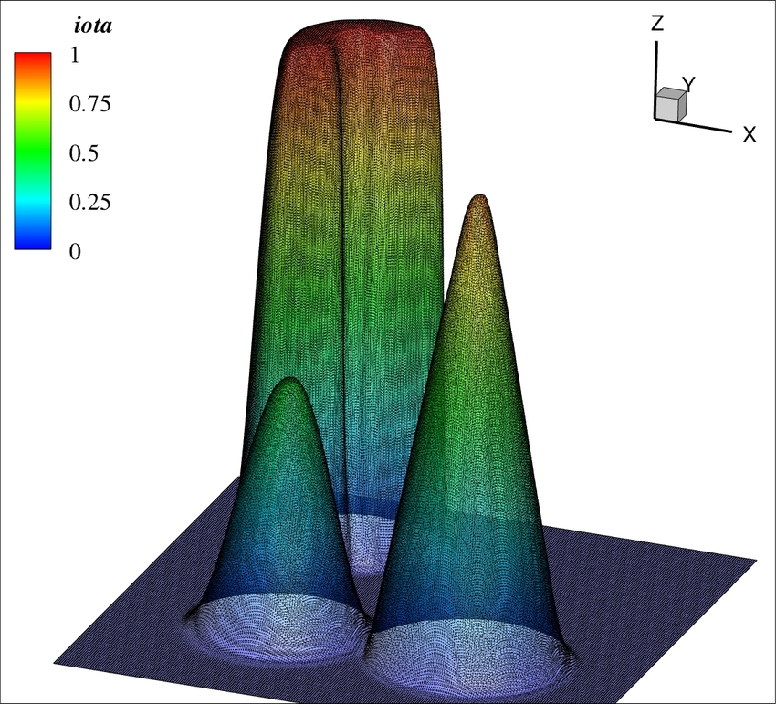
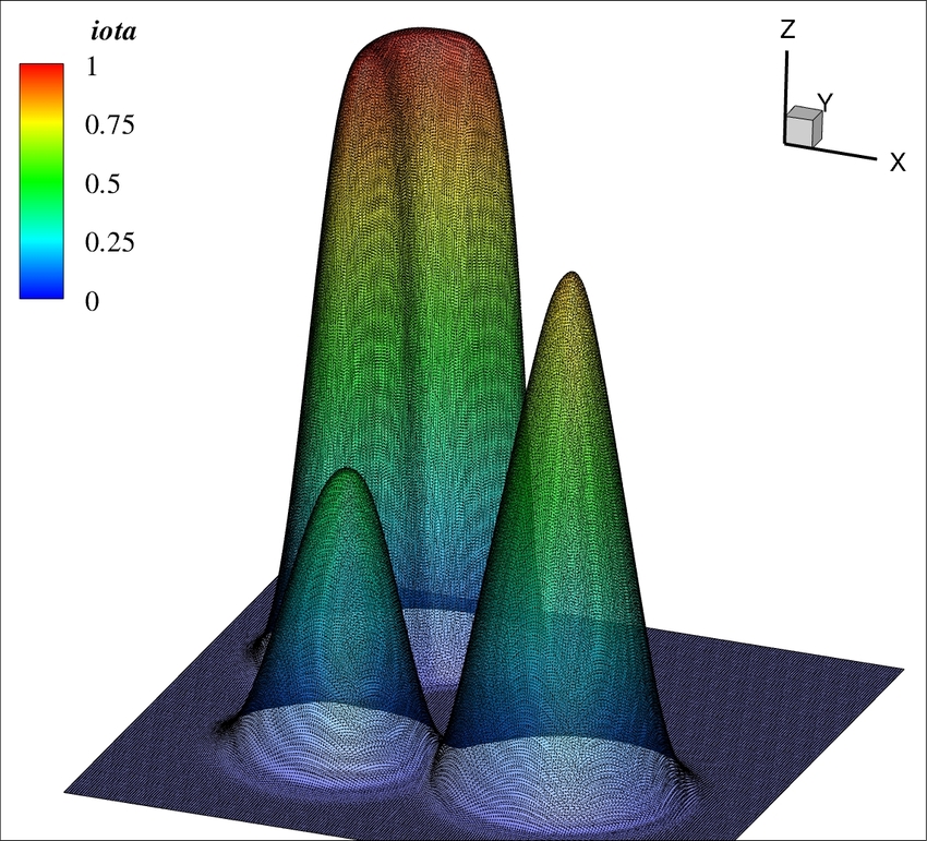
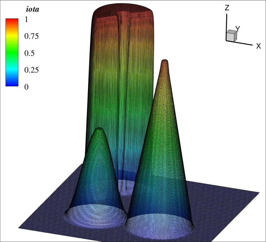
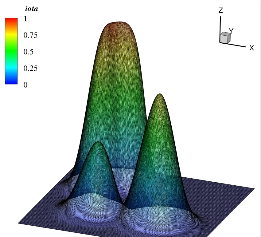
The outline of this paper is as follows. In §2 we present our generalized setting, which can be summarized as: given an advection-diffusion system of equations, consider the initial free boundary value problem recast into the weak formulation and spatially discretized. We then take a temporal discretization via a RKSSP DG approach in which we obtain the form of our approximate solutions. Our formulation is general, while our examples focus on problems of hyperbolic transport saving the more general applications for the sequel to this paper. In §3 we introduce a number of slope limiters consistent with any order p𝑝p basis. The first is the vertex limiter regime of [25], the second the classical Barth–Jespersen limiter [6], and the third and fourth are minor adaptations of the former two limiters made with an eye towards improving the L2superscript𝐿2L^{2}–error convergence by adjusting a so–called “blind spot” present in the previous schemes at higher order p𝑝p. The fifth approach is comprised of a family of hierarchical reconstruction approaches [1, 27], while the sixth regime is a linear restriction method that can be viewed as a generalization of a limiter originally sketched in [7]. The final limiting regime we present is a mixed extension of the previous limiters referred to here as a hierarchic recombination approach. Section §4 then provides numerical experimentation using the schemes presented in §3 – namely a classical advective scalar transport problem, and a stationary solution to a closely related problem with highly singular initial data. We also show some convergence results on an analytic test case. Finally, in §5 we present the adaptive p𝑝p-enrichment schemes, which are fully coupled to the slope limiters from §4 ab initio. These come in two basic types, the first for (heuristically) smooth solutions, and the second for solutions demonstrating (vaguely) “appreciable gradients.”

2 §​2§2\S 2 Advection–diffusion systems in the DG formalism

We are interested in solutions to an initial-boundary value problem for a generalized advection-diffusion system of arbitrarily mixed hyperbolic-parabolic type in Ω×(0,T)Ω0𝑇\Omega\times(0,T), where Ω⊂ℝ2Ωsuperscriptℝ2\Omega\subset\mathbb{R}^{2} with boundary ∂ΩΩ\partial\Omega, such that the system satisfies:

đ‘Œt+𝑭x−𝑼x=𝒈,given​initial​conditionsđ‘Œ|t=0=đ‘Œ0,\boldsymbol{U}_{t}+\boldsymbol{F}_{x}-\boldsymbol{G}_{x}=\boldsymbol{g},\quad\mathrm{given\ initial\ conditions}\quad\boldsymbol{U}_{|t=0}=\boldsymbol{U}_{0}, (2.1)

and generalized componentwise Robin boundary values

ai​Ui+∇xUi,x​(bi⋅𝒏+ci⋅𝝉)−fi=0,on​∂Ω.subscript𝑎𝑖subscript𝑈𝑖subscriptâˆ‡đ‘„subscriptđ‘ˆđ‘–đ‘„â‹…subscript𝑏𝑖𝒏⋅subscript𝑐𝑖𝝉subscript𝑓𝑖0onΩa_{i}U_{i}+\nabla_{x}U_{i,x}\left(b_{i}\cdot\boldsymbol{n}+c_{i}\cdot\boldsymbol{\tau}\right)-f_{i}=0,\quad\mathrm{on}\ \partial\Omega. (2.2)

That is, the system is comprised of a generalized m𝑚m-dimensional state vector đ‘Œ=đ‘Œâ€‹(t,𝒙)=(U1,
,Um)đ‘Œđ‘Œđ‘Ąđ’™subscript𝑈1
subscript𝑈𝑚\boldsymbol{U}=\boldsymbol{U}(t,\boldsymbol{x})=(U_{1},\ldots,U_{m}), an advective flux matrix 𝑭=𝑭​(đ‘Œ)đ‘­đ‘­đ‘Œ\boldsymbol{F}=\boldsymbol{F}(\boldsymbol{U}), a viscous flux matrix 𝑼=𝑼​(đ‘Œ,đ‘Œx)đ‘źđ‘źđ‘Œsubscriptđ‘Œđ‘„\boldsymbol{G}=\boldsymbol{G}(\boldsymbol{U},\boldsymbol{U}_{x}), and a source term 𝒈=𝒈​(t,𝒙)=(g1,
,gm)𝒈𝒈𝑡𝒙subscript𝑔1
subscript𝑔𝑚\boldsymbol{g}=\boldsymbol{g}(t,\boldsymbol{x})=(g_{1},\ldots,g_{m}), where 𝒙∈ℝ2𝒙superscriptℝ2\boldsymbol{x}\in\mathbb{R}^{2} and t∈(0,T)𝑡0𝑇t\in(0,T). The vectors 𝒂𝒂\boldsymbol{a}, 𝒃𝒃\boldsymbol{b}, 𝒄𝒄\boldsymbol{c} and 𝒇𝒇\boldsymbol{f} are comprised of the m𝑚m functions, ai=ai​(t,𝒙)subscript𝑎𝑖subscript𝑎𝑖𝑡𝒙a_{i}=a_{i}(t,\boldsymbol{x}), bi=bi​(t,𝒙)subscript𝑏𝑖subscript𝑏𝑖𝑡𝒙b_{i}=b_{i}(t,\boldsymbol{x}), ci=ci​(t,𝒙)subscript𝑐𝑖subscript𝑐𝑖𝑡𝒙c_{i}=c_{i}(t,\boldsymbol{x}) and fi=fi​(t,𝒙)subscript𝑓𝑖subscript𝑓𝑖𝑡𝒙f_{i}=f_{i}(t,\boldsymbol{x}) for i=1,
,m𝑖1
𝑚i=1,\ldots,m, where 𝒏𝒏\boldsymbol{n} denotes the unit outward pointing normal and 𝝉𝝉\boldsymbol{\tau} the unit tangent vector.

In addition, because we are interested in approximate numerical solutions of the form of [2, 3] restricted in part to the family of methods for elliptic equations, we rewrite (2.1) as a coupled system in terms of an auxiliary variable đšșđšș\boldsymbol{\Sigma}, such that

đ‘Œt+𝑭x−𝑼x=𝒈,andđšș=đ‘Œx,formulae-sequencesubscriptđ‘Œđ‘Ąsubscriptđ‘­đ‘„subscriptđ‘źđ‘„đ’ˆandđšșsubscriptđ‘Œđ‘„\displaystyle\boldsymbol{U}_{t}+\boldsymbol{F}_{x}-\boldsymbol{G}_{x}=\boldsymbol{g},\quad\mathrm{and}\quad\boldsymbol{\Sigma}=\boldsymbol{U}_{x}, (2.3)

where we have substituted in the viscous flux matrix the auxiliary term, so that 𝑼=𝑼​(đ‘Œ,đšș)đ‘źđ‘źđ‘Œđšș\boldsymbol{G}=\boldsymbol{G}(\boldsymbol{U},\boldsymbol{\Sigma}).

For notational completeness we adopt the following discretization scheme motivated by [31, 13]. Take an open Ω⊂ℝ2Ωsuperscriptℝ2\Omega\subset\mathbb{R}^{2} with boundary ∂ΩΩ\partial\Omega, given T>0𝑇0T>0 such that 𝒬T=((0,T)×Ω)subscript𝒬𝑇0đ‘‡Î©\mathcal{Q}_{T}=((0,T)\times\Omega). Let 𝒯hsubscript𝒯ℎ\mathscr{T}_{h} denote the partition of the closure of the polygonal triangulation of ΩΩ\Omega, which we denote ΩhsubscriptΩℎ\Omega_{h}, into a finite number of polygonal elements denoted ΩesubscriptÎ©đ‘’\Omega_{e}, such that 𝒯h={Ωe1,Ωe2,
,Ωen​e}subscript𝒯ℎsubscriptΩsubscript𝑒1subscriptΩsubscript𝑒2
subscriptΩsubscript𝑒𝑛𝑒\mathscr{T}_{h}=\{\Omega_{e_{1}},\Omega_{e_{2}},\ldots,\Omega_{e_{ne}}\}, for n​e∈ℕ𝑛𝑒ℕne\in\mathbb{N} the number of elements in ΩhsubscriptΩℎ\Omega_{h}. In this work we define the mesh diameter hℎh to satisfy h=mini​j⁥(di​j)ℎsubscript𝑖𝑗subscript𝑑𝑖𝑗h=\min_{ij}(d_{ij}) for the distance function di​j=d​(𝒙i,𝒙j)subscript𝑑𝑖𝑗𝑑subscript𝒙𝑖subscript𝒙𝑗d_{ij}=d(\boldsymbol{x}_{i},\boldsymbol{x}_{j}) and elementwise edge vertices 𝒙i,𝒙j∈∂Ωesubscript𝒙𝑖subscript𝒙𝑗subscriptÎ©đ‘’\boldsymbol{x}_{i},\boldsymbol{x}_{j}\in\partial\Omega_{e} when the mesh is structured and regular. For unstructured meshes we mean the average value of hℎh over the mesh.

Now, let Γi​jsubscriptΓ𝑖𝑗\Gamma_{ij} denote the edge shared by two neighboring elements ΩeisubscriptΩsubscript𝑒𝑖\Omega_{e_{i}} and ΩejsubscriptΩsubscript𝑒𝑗\Omega_{e_{j}}, and for i∈I⊂℀+={1,2,
}đ‘–đŒsuperscriptâ„€12
i\in I\subset\mathbb{Z}^{+}=\{1,2,\ldots\} define the indexing set r(i)={j∈I:Ωejr(i)=\{j\in I:\Omega_{e_{j}} is a neighbor of Ωei}\Omega_{e_{i}}\}. Let us denote all ΩeisubscriptΩsubscript𝑒𝑖\Omega_{e_{i}} containing the boundary ∂ΩhsubscriptΩℎ\partial\Omega_{h} by Sjsubscript𝑆𝑗S_{j} and letting IB⊂℀−={−1,−2,
}subscriptđŒđ”superscriptâ„€12
I_{B}\subset\mathbb{Z}^{-}=\{-1,-2,\ldots\} define s(i)={j∈IB:Sjs(i)=\{j\in I_{B}:S_{j} is an edge of Ωei}\Omega_{e_{i}}\} such that Γi​j=SjsubscriptΓ𝑖𝑗subscript𝑆𝑗\Gamma_{ij}=S_{j} for Ωei∈ΩhsubscriptΩsubscript𝑒𝑖subscriptΩℎ\Omega_{e_{i}}\in\Omega_{h} when Sj∈∂Ωeisubscript𝑆𝑗subscriptΩsubscript𝑒𝑖S_{j}\in\partial\Omega_{e_{i}}, j∈IB𝑗subscriptđŒđ”j\in I_{B}. Then for Ξi=r​(i)âˆȘs​(i)subscriptΞ𝑖𝑟𝑖𝑠𝑖\Xi_{i}=r(i)\cup s(i), we have

∂Ωei=⋃j∈Ξ​(i)Γi​j,and∂Ωei∩∂Ωh=⋃j∈s​(i)Γi​j.formulae-sequencesubscriptΩsubscript𝑒𝑖subscript𝑗Ξ𝑖subscriptΓ𝑖𝑗andsubscriptΩsubscript𝑒𝑖subscriptΩℎsubscript𝑗𝑠𝑖subscriptΓ𝑖𝑗\partial\Omega_{e_{i}}=\bigcup_{j\in\Xi(i)}\Gamma_{ij},\quad\mathrm{and}\quad\partial\Omega_{e_{i}}\cap\partial\Omega_{h}=\bigcup_{j\in s(i)}\Gamma_{ij}.

We are interested in obtaining an approximate solution to đ‘Œđ‘Œ\boldsymbol{U} at time t𝑡t on the finite dimensional space of discontinuous piecewise polynomial functions over ΩΩ\Omega restricted to 𝒯hsubscript𝒯ℎ\mathscr{T}_{h}, given as

Shp​(Ωh,𝒯h)={v:v|Ωeiâˆˆđ’«p​(Ωei)∀Ωei∈𝒯h}S_{h}^{p}(\Omega_{h},\mathscr{T}_{h})=\{v:v_{|\Omega_{e_{i}}}\in\mathscr{P}^{p}(\Omega_{e_{i}})\ \ \forall\Omega_{e_{i}}\in\mathscr{T}_{h}\}

for đ’«p​(Ωei)superscriptđ’«đ‘subscriptΩsubscript𝑒𝑖\mathscr{P}^{p}(\Omega_{e_{i}}) the space of degree ≀pabsent𝑝\leq p polynomials over ΩeisubscriptΩsubscript𝑒𝑖\Omega_{e_{i}}.

Choosing a set of degree p𝑝p polynomial basis functions Nâ„“âˆˆđ’«p​(Ωei)subscript𝑁ℓsuperscriptđ’«đ‘subscriptΩsubscript𝑒𝑖N_{\ell}\in\mathscr{P}^{p}(\Omega_{e_{i}}) for ℓ=1,
,npℓ1
subscript𝑛𝑝\ell=1,\ldots,n_{p} corresponding to the degree of freedom, we can denote the state vector at time t𝑡t over ΩeisubscriptΩsubscript𝑒𝑖\Omega_{e_{i}}, by

đ‘Œh​(t,𝒙)=∑ℓ=1npđ‘Œâ„“i​(t)​Nℓi​(𝒙),∀x∈Ωei,formulae-sequencesubscriptđ‘Œâ„Žđ‘Ąđ’™superscriptsubscriptℓ1subscript𝑛𝑝superscriptsubscriptđ‘Œâ„“đ‘–đ‘Ąsubscriptsuperscript𝑁𝑖ℓ𝒙for-allđ‘„subscriptΩsubscript𝑒𝑖\boldsymbol{U}_{h}(t,\boldsymbol{x})=\sum_{\ell=1}^{n_{p}}\boldsymbol{U}_{\ell}^{i}(t)N^{i}_{\ell}(\boldsymbol{x}),\quad\forall x\in\Omega_{e_{i}}, (2.4)

where the Nℓisubscriptsuperscript𝑁𝑖ℓN^{i}_{\ell}’s are the finite element shape functions in the DG setting, and the đ‘Œâ„“isuperscriptsubscriptđ‘Œâ„“đ‘–\boldsymbol{U}_{\ell}^{i}’s correspond to the unknowns. We characterize the finite dimensional test functions

𝒗h,𝝎h∈Wk,q​(Ωh,𝒯h),by𝒗h​(x)=∑ℓ=1np𝒗ℓi​Nℓi​(x)and𝝎h​(x)=∑ℓ=1np𝝎ℓi​Nℓi​(x)formulae-sequencesubscript𝒗ℎsubscript𝝎ℎsuperscript𝑊𝑘𝑞subscriptΩℎsubscript𝒯ℎbysubscriptđ’—â„Žđ‘„superscriptsubscriptℓ1subscript𝑛𝑝superscriptsubscript𝒗ℓ𝑖superscriptsubscriptđ‘â„“đ‘–đ‘„andsubscriptđŽâ„Žđ‘„superscriptsubscriptℓ1subscript𝑛𝑝superscriptsubscript𝝎ℓ𝑖superscriptsubscriptđ‘â„“đ‘–đ‘„\displaystyle\boldsymbol{v}_{h},\boldsymbol{\omega}_{h}\in W^{k,q}(\Omega_{h},\mathscr{T}_{h}),\quad\mathrm{by}\quad\boldsymbol{v}_{h}(x)=\sum_{\ell=1}^{n_{p}}\boldsymbol{v}_{\ell}^{i}N_{\ell}^{i}(x)\quad\mathrm{and}\quad\boldsymbol{\omega}_{h}(x)=\sum_{\ell=1}^{n_{p}}\boldsymbol{\omega}_{\ell}^{i}N_{\ell}^{i}(x)

where 𝒗ℓisuperscriptsubscript𝒗ℓ𝑖\boldsymbol{v}_{\ell}^{i} and 𝝎ℓisuperscriptsubscript𝝎ℓ𝑖\boldsymbol{\omega}_{\ell}^{i} are the coordinates of the test functions in each ΩeisubscriptΩsubscript𝑒𝑖\Omega_{e_{i}}, and with the broken Sobolev space over the partition 𝒯hsubscript𝒯ℎ\mathscr{T}_{h} defined by

Wk,q​(Ωh,𝒯h)={w:w|Ωei∈Wk,q​(Ωei)∀Ωei∈𝒯h}.W^{k,q}(\Omega_{h},\mathscr{T}_{h})=\{w:w_{|\Omega_{e_{i}}}\in W^{k,q}(\Omega_{e_{i}})\ \ \forall\Omega_{e_{i}}\in\mathscr{T}_{h}\}.

Thus, for đ‘Œđ‘Œ\boldsymbol{U} a classical solution to (2.3), multiplying by 𝒗hsubscript𝒗ℎ\boldsymbol{v}_{h} or 𝝎hsubscript𝝎ℎ\boldsymbol{\omega}_{h} and integrating elementwise by parts yields the coupled system:

dd​t​∫Ωeiđ‘Œâ‹…đ’—h​𝑑x+∫Ωei(𝑭⋅𝒗h)x​𝑑x−∫Ωei𝑭:𝒗xh​d​x:𝑑𝑑𝑡subscriptsubscriptΩsubscriptđ‘’đ‘–â‹…đ‘Œsubscript𝒗ℎdifferential-dđ‘„subscriptsubscriptΩsubscript𝑒𝑖subscript⋅𝑭subscriptđ’—â„Žđ‘„differential-dđ‘„subscriptsubscriptΩsubscript𝑒𝑖𝑭subscriptsuperscriptđ’—â„Žđ‘„đ‘‘đ‘„\displaystyle\frac{d}{dt}\int_{\Omega_{e_{i}}}\boldsymbol{U}\cdot\boldsymbol{v}_{h}dx+\int_{\Omega_{e_{i}}}(\boldsymbol{F}\cdot\boldsymbol{v}_{h})_{x}dx-\int_{\Omega_{e_{i}}}\boldsymbol{F}:\boldsymbol{v}^{h}_{x}dx (2.5)
−∫Ωei(𝑼⋅𝒗h)x​𝑑x+∫Ωei𝑼:𝒗xh​d​x=∫Ωei𝒗h⋅𝒈​𝑑x,:subscriptsubscriptΩsubscript𝑒𝑖subscript⋅𝑼subscriptđ’—â„Žđ‘„differential-dđ‘„subscriptsubscriptΩsubscript𝑒𝑖𝑼subscriptsuperscriptđ’—â„Žđ‘„đ‘‘đ‘„subscriptsubscriptΩsubscript𝑒𝑖⋅subscript𝒗ℎ𝒈differential-dđ‘„\displaystyle\qquad\qquad-\int_{\Omega_{e_{i}}}(\boldsymbol{G}\cdot\boldsymbol{v}_{h})_{x}dx+\int_{\Omega_{e_{i}}}\boldsymbol{G}:\boldsymbol{v}^{h}_{x}dx=\int_{\Omega_{e_{i}}}\boldsymbol{v}_{h}\cdot\boldsymbol{g}dx,
∫Ωeiđšș⋅𝝎h​𝑑x−∫Ωei(đ‘Œâ‹…đŽh)x​𝑑x+∫Ωeiđ‘Œ:𝝎xh​d​x=0,:subscriptsubscriptΩsubscript𝑒𝑖⋅đšșsubscript𝝎ℎdifferential-dđ‘„subscriptsubscriptΩsubscript𝑒𝑖subscriptâ‹…đ‘ŒsubscriptđŽâ„Žđ‘„differential-dđ‘„subscriptsubscriptΩsubscriptđ‘’đ‘–đ‘ŒsubscriptsuperscriptđŽâ„Žđ‘„đ‘‘đ‘„0\displaystyle\int_{\Omega_{e_{i}}}\boldsymbol{\Sigma}\cdot\boldsymbol{\omega}_{h}dx-\int_{\Omega_{e_{i}}}(\boldsymbol{U}\cdot\boldsymbol{\omega}_{h})_{x}dx+\int_{\Omega_{e_{i}}}\boldsymbol{U}:\boldsymbol{\omega}^{h}_{x}dx=0,

where (:):(:) denotes the scalar product.

Now, let 𝒏i​jsubscript𝒏𝑖𝑗\boldsymbol{n}_{ij} be the unit outward normal to ∂ΩeisubscriptΩsubscript𝑒𝑖\partial\Omega_{e_{i}} on Γi​jsubscriptΓ𝑖𝑗\Gamma_{ij}, and let v|Γi​jv_{|\Gamma_{ij}} and v|Γj​iv_{|\Gamma_{ji}} denote the values of v𝑣v on Γi​jsubscriptΓ𝑖𝑗\Gamma_{ij} considered from the interior and the exterior of ΩeisubscriptΩsubscript𝑒𝑖\Omega_{e_{i}}, respectively. Then by choosing componentwise approximations in (LABEL:approxsystem) by substituting in (2.4), we arrive with the approximate form of the first term of (LABEL:approxsystem) given by,

dd​t​∫Ωeiđ‘Œh⋅𝒗h​𝑑x≈dd​t​∫Ωeiđ‘Œâ‹…đ’—h​𝑑x,𝑑𝑑𝑡subscriptsubscriptΩsubscript𝑒𝑖⋅subscriptđ‘Œâ„Žsubscript𝒗ℎdifferential-dđ‘„đ‘‘đ‘‘đ‘ĄsubscriptsubscriptΩsubscriptđ‘’đ‘–â‹…đ‘Œsubscript𝒗ℎdifferential-dđ‘„\displaystyle\frac{d}{dt}\int_{\Omega_{e_{i}}}\boldsymbol{U}_{h}\cdot\boldsymbol{v}_{h}dx\approx\frac{d}{dt}\int_{\Omega_{e_{i}}}\boldsymbol{U}\cdot\boldsymbol{v}_{h}dx, (2.6)

the second term using an inviscid numerical flux đšœisubscriptđšœđ‘–\boldsymbol{\Phi}_{i}, by

đšœ~i​(đ‘Œh|Γi​j,đ‘Œh|Γj​i,𝒗h)subscript~đšœđ‘–evaluated-atsubscriptđ‘Œâ„ŽsubscriptΓ𝑖𝑗evaluated-atsubscriptđ‘Œâ„ŽsubscriptΓ𝑗𝑖subscript𝒗ℎ\displaystyle\tilde{\boldsymbol{\Phi}}_{i}(\boldsymbol{U}_{h}|_{\Gamma_{ij}},\boldsymbol{U}_{h}|_{\Gamma_{ji}},\boldsymbol{v}_{h}) =∑j∈Ξ​(i)∫Γi​jđšœâ€‹(đ‘Œh|Γi​j,đ‘Œh|Γj​i,𝒏i​j)⋅𝒗h|Γi​j​d​Ξabsentevaluated-atsubscript𝑗Ξ𝑖subscriptsubscriptÎ“đ‘–đ‘—â‹…đšœevaluated-atsubscriptđ‘Œâ„ŽsubscriptΓ𝑖𝑗evaluated-atsubscriptđ‘Œâ„ŽsubscriptΓ𝑗𝑖subscript𝒏𝑖𝑗subscript𝒗ℎsubscriptΓ𝑖𝑗𝑑Ξ\displaystyle=\sum_{j\in\Xi(i)}\int_{\Gamma_{ij}}\boldsymbol{\Phi}(\boldsymbol{U}_{h}|_{\Gamma_{ij}},\boldsymbol{U}_{h}|_{\Gamma_{ji}},\boldsymbol{n}_{ij})\cdot\boldsymbol{v}_{h}|_{\Gamma_{ij}}d\Xi (2.7)
≈∑j∈Ξ​(i)∫Γi​j∑l=12(𝑭)l⋅(ni​j)l​𝒗h|Γi​j​d​Ξ,absentevaluated-atsubscript𝑗Ξ𝑖subscriptsubscriptΓ𝑖𝑗superscriptsubscript𝑙12⋅subscript𝑭𝑙subscriptsubscript𝑛𝑖𝑗𝑙subscript𝒗ℎsubscriptΓ𝑖𝑗𝑑Ξ\displaystyle\approx\sum_{j\in\Xi(i)}\int_{\Gamma_{ij}}\sum_{l=1}^{2}(\boldsymbol{F})_{l}\cdot(n_{ij})_{l}\boldsymbol{v}_{h}|_{\Gamma_{ij}}d\Xi,

and the third term in (LABEL:approxsystem) by,

𝚯i​(đ‘Œh,𝒗h)=∫Ωei𝑭h:𝒗xh​d​x≈∫Ωei𝑭:𝒗xh​d​x.:subscript𝚯𝑖subscriptđ‘Œâ„Žsubscript𝒗ℎsubscriptsubscriptΩsubscript𝑒𝑖subscript𝑭ℎsubscriptsuperscriptđ’—â„Žđ‘„đ‘‘đ‘„subscriptsubscriptΩsubscript𝑒𝑖𝑭:subscriptsuperscriptđ’—â„Žđ‘„đ‘‘đ‘„\boldsymbol{\Theta}_{i}(\boldsymbol{U}_{h},\boldsymbol{v}_{h})=\int_{\Omega_{e_{i}}}\boldsymbol{F}_{h}:\boldsymbol{v}^{h}_{x}dx\approx\int_{\Omega_{e_{i}}}\boldsymbol{F}:\boldsymbol{v}^{h}_{x}dx. (2.8)

Next we approximate the boundary viscous term of (LABEL:approxsystem) using a generalized viscous flux 𝒱^^𝒱\hat{\mathscr{G}} such that,

𝒱i​(đšșh,đ‘Œh,𝒗h)subscript𝒱𝑖subscriptđšșℎsubscriptđ‘Œâ„Žsubscript𝒗ℎ\displaystyle\mathscr{G}_{i}(\boldsymbol{\Sigma}_{h},\boldsymbol{U}_{h},\boldsymbol{v}_{h}) =∑j∈Ξ​(i)∫Γi​j𝒱^​(đšșh|Γi​j,đšșh|Γj​i,đ‘Œh|Γi​j,đ‘Œh|Γj​i,𝒏i​j)⋅𝒗h|Γi​j​d​Ξabsentevaluated-atsubscript𝑗Ξ𝑖subscriptsubscriptΓ𝑖𝑗⋅^𝒱evaluated-atsubscriptđšșℎsubscriptΓ𝑖𝑗evaluated-atsubscriptđšșℎsubscriptΓ𝑗𝑖evaluated-atsubscriptđ‘Œâ„ŽsubscriptΓ𝑖𝑗evaluated-atsubscriptđ‘Œâ„ŽsubscriptΓ𝑗𝑖subscript𝒏𝑖𝑗subscript𝒗ℎsubscriptΓ𝑖𝑗𝑑Ξ\displaystyle=\sum_{j\in\Xi(i)}\int_{\Gamma_{ij}}\hat{\mathscr{G}}(\boldsymbol{\Sigma}_{h}|_{\Gamma_{ij}},\boldsymbol{\Sigma}_{h}|_{\Gamma_{ji}},\boldsymbol{U}_{h}|_{\Gamma_{ij}},\boldsymbol{U}_{h}|_{\Gamma_{ji}},\boldsymbol{n}_{ij})\cdot\boldsymbol{v}_{h}|_{\Gamma_{ij}}d\Xi (2.9)
≈∑j∈Ξ​(i)∫Γi​j∑l=12(𝑼)l⋅(ni​j)l​𝒗h|Γi​j​d​Ξ,absentevaluated-atsubscript𝑗Ξ𝑖subscriptsubscriptΓ𝑖𝑗superscriptsubscript𝑙12⋅subscript𝑼𝑙subscriptsubscript𝑛𝑖𝑗𝑙subscript𝒗ℎsubscriptΓ𝑖𝑗𝑑Ξ\displaystyle\approx\sum_{j\in\Xi(i)}\int_{\Gamma_{ij}}\sum_{l=1}^{2}(\boldsymbol{G})_{l}\cdot(n_{ij})_{l}\boldsymbol{v}_{h}|_{\Gamma_{ij}}d\Xi,

while the second viscous term is approximated by:

đ’©i​(đšșh,đ‘Œh,𝒗h)=∫Ωei𝑼h:𝒗xh​d​x≈∫Ωei𝑼:𝒗xh​d​x.:subscriptđ’©đ‘–subscriptđšșℎsubscriptđ‘Œâ„Žsubscript𝒗ℎsubscriptsubscriptΩsubscript𝑒𝑖subscript𝑼ℎsubscriptsuperscriptđ’—â„Žđ‘„đ‘‘đ‘„subscriptsubscriptΩsubscript𝑒𝑖𝑼:subscriptsuperscriptđ’—â„Žđ‘„đ‘‘đ‘„\mathscr{N}_{i}(\boldsymbol{\Sigma}_{h},\boldsymbol{U}_{h},\boldsymbol{v}_{h})=\int_{\Omega_{e_{i}}}\boldsymbol{G}_{h}:\boldsymbol{v}^{h}_{x}dx\approx\int_{\Omega_{e_{i}}}\boldsymbol{G}:\boldsymbol{v}^{h}_{x}dx. (2.10)

Finally the source 𝒈𝒈\boldsymbol{g} term of (LABEL:approxsystem) is given to satisfy

ℋi​(𝒗h,𝒙h,t)=∫Ωei𝒗h⋅𝒈h​𝑑x≈∫Ωei𝒗h⋅𝒈​𝑑x.subscriptℋ𝑖subscript𝒗ℎsubscript𝒙ℎ𝑡subscriptsubscriptΩsubscript𝑒𝑖⋅subscript𝒗ℎsubscript𝒈ℎdifferential-dđ‘„subscriptsubscriptΩsubscript𝑒𝑖⋅subscript𝒗ℎ𝒈differential-dđ‘„\displaystyle\mathscr{H}_{i}(\boldsymbol{v}_{h},\boldsymbol{x}_{h},t)=\int_{\Omega_{e_{i}}}\boldsymbol{v}_{h}\cdot\boldsymbol{g}_{h}dx\approx\int_{\Omega_{e_{i}}}\boldsymbol{v}_{h}\cdot\boldsymbol{g}dx. (2.11)

For the auxiliary equation in (LABEL:approxsystem) we expand it such that the approximate solution satisfies:

𝒬i​(đ‘Œ^,đšșh,đ‘Œh,𝝎h,𝝎xh)subscript𝒬𝑖^đ‘Œsubscriptđšșℎsubscriptđ‘Œâ„Žsubscript𝝎ℎsuperscriptsubscriptđŽđ‘„â„Ž\displaystyle\mathscr{Q}_{i}(\hat{\boldsymbol{U}},\boldsymbol{\Sigma}_{h},\boldsymbol{U}_{h},\boldsymbol{\omega}_{h},\boldsymbol{\omega}_{x}^{h}) =∫Ωeiđšșh⋅𝝎h​𝑑x+∫Ωeiđ‘Œh:𝝎xh​d​x:absentsubscriptsubscriptΩsubscript𝑒𝑖⋅subscriptđšșℎsubscript𝝎ℎdifferential-dđ‘„subscriptsubscriptΩsubscript𝑒𝑖subscriptđ‘Œâ„ŽsubscriptsuperscriptđŽâ„Žđ‘„đ‘‘đ‘„\displaystyle=\int_{\Omega_{e_{i}}}\boldsymbol{\Sigma}_{h}\cdot\boldsymbol{\omega}_{h}dx+\int_{\Omega_{e_{i}}}\boldsymbol{U}_{h}:\boldsymbol{\omega}^{h}_{x}dx (2.12)
−∑j∈Ξ​(i)∫Γi​jđ‘Œ^​(đ‘Œh|Γi​j,đ‘Œh|Γj​i,𝝎h|Γi​j,𝒏i​j)​𝑑Ξ=0,subscript𝑗Ξ𝑖subscriptsubscriptΓ𝑖𝑗^đ‘Œevaluated-atsubscriptđ‘Œâ„ŽsubscriptΓ𝑖𝑗evaluated-atsubscriptđ‘Œâ„ŽsubscriptΓ𝑗𝑖evaluated-atsubscript𝝎ℎsubscriptΓ𝑖𝑗subscript𝒏𝑖𝑗differential-dΞ0\displaystyle-\sum_{j\in\Xi(i)}\int_{\Gamma_{ij}}\hat{\boldsymbol{U}}(\boldsymbol{U}_{h}|_{\Gamma_{ij}},\boldsymbol{U}_{h}|_{\Gamma_{ji}},\boldsymbol{\omega}_{h}|_{\Gamma_{ij}},\boldsymbol{n}_{ij})d\Xi=0,

where,

∑i∈I∑j∈Ξ​(i)∫Γi​jđ‘Œ^​(đ‘Œh|Γi​j,đ‘Œh|Γj​i,𝝎h|Γi​j,𝒏i​j)​𝑑Ξ≈∑i∈I∑j∈Ξ​(i)∫Γi​j∑l=12(đ‘Œ)l⋅(ni​j)l​𝝎h|Γi​j​d​Ξsubscriptđ‘–đŒsubscript𝑗Ξ𝑖subscriptsubscriptΓ𝑖𝑗^đ‘Œevaluated-atsubscriptđ‘Œâ„ŽsubscriptΓ𝑖𝑗evaluated-atsubscriptđ‘Œâ„ŽsubscriptΓ𝑗𝑖evaluated-atsubscript𝝎ℎsubscriptΓ𝑖𝑗subscript𝒏𝑖𝑗differential-dΞevaluated-atsubscriptđ‘–đŒsubscript𝑗Ξ𝑖subscriptsubscriptΓ𝑖𝑗superscriptsubscript𝑙12⋅subscriptđ‘Œđ‘™subscriptsubscript𝑛𝑖𝑗𝑙subscript𝝎ℎsubscriptΓ𝑖𝑗𝑑Ξ\displaystyle\sum_{i\in I}\sum_{j\in\Xi(i)}\int_{\Gamma_{ij}}\hat{\boldsymbol{U}}(\boldsymbol{U}_{h}|_{\Gamma_{ij}},\boldsymbol{U}_{h}|_{\Gamma_{ji}},\boldsymbol{\omega}_{h}|_{\Gamma_{ij}},\boldsymbol{n}_{ij})d\Xi\approx\sum_{i\in I}\sum_{j\in\Xi(i)}\int_{\Gamma_{ij}}\sum_{l=1}^{2}(\boldsymbol{U})_{l}\cdot(n_{ij})_{l}\boldsymbol{\omega}_{h}|_{\Gamma_{ij}}d\Xi

given đ‘Œ^^đ‘Œ\hat{\boldsymbol{U}} a generalized numerical flux, and where

∫Ωeiđšșh⋅𝝎h​𝑑x≈∫Ωeiđšș⋅𝝎h​𝑑x,and∫Ωeiđ‘Œh:𝝎xh​d​x≈∫Ωeiđ‘Œ:𝝎xh​d​x.:subscriptsubscriptΩsubscript𝑒𝑖⋅subscriptđšșℎsubscript𝝎ℎdifferential-dđ‘„subscriptsubscriptΩsubscript𝑒𝑖⋅đšșsubscript𝝎ℎdifferential-dđ‘„andsubscriptsubscriptΩsubscript𝑒𝑖subscriptđ‘Œâ„ŽsubscriptsuperscriptđŽâ„Žđ‘„đ‘‘đ‘„subscriptsubscriptΩsubscriptđ‘’đ‘–đ‘Œ:subscriptsuperscriptđŽâ„Žđ‘„đ‘‘đ‘„\int_{\Omega_{e_{i}}}\boldsymbol{\Sigma}_{h}\cdot\boldsymbol{\omega}_{h}dx\approx\int_{\Omega_{e_{i}}}\boldsymbol{\Sigma}\cdot\boldsymbol{\omega}_{h}dx,\quad\mathrm{and}\quad\int_{\Omega_{e_{i}}}\boldsymbol{U}_{h}:\boldsymbol{\omega}^{h}_{x}dx\approx\int_{\Omega_{e_{i}}}\boldsymbol{U}:\boldsymbol{\omega}^{h}_{x}dx.

Combining the above approximations and setting, 𝒳=∑Ωei∈𝒯h𝒳i𝒳subscriptsubscriptΩsubscript𝑒𝑖subscript𝒯ℎsubscript𝒳𝑖\mathscr{X}=\sum_{\Omega_{e_{i}}\in\mathscr{T}_{h}}\mathscr{X}_{i}, while denoting the inner product

(𝒂hn,𝒃h)Î©đ’ą=∑Ωei∈𝒯h∫Ωei𝒂hn⋅𝒃h​𝑑x,subscriptsuperscriptsubscript𝒂ℎ𝑛subscript𝒃ℎsubscriptÎ©đ’ąsubscriptsubscriptΩsubscript𝑒𝑖subscript𝒯ℎsubscriptsubscriptΩsubscript𝑒𝑖⋅superscriptsubscript𝒂ℎ𝑛subscript𝒃ℎdifferential-dđ‘„(\boldsymbol{a}_{h}^{n},\boldsymbol{b}_{h})_{\Omega_{\mathcal{G}}}=\sum_{\Omega_{e_{i}}\in\mathscr{T}_{h}}\int_{\Omega_{e_{i}}}\boldsymbol{a}_{h}^{n}\cdot\boldsymbol{b}_{h}dx,

we arrive at our approximate solution to (2.3) as the pair of functions (đ‘Œh,đšșh)subscriptđ‘Œâ„Žsubscriptđšșℎ(\boldsymbol{U}_{h},\boldsymbol{\Sigma}_{h}) for all t∈(0,T)𝑡0𝑇t\in(0,T) satisfying:

The Discontinuous Galerkin formulation

a)đ‘Œh∈C1((0,T);Shp),đšșh∈Shp,\displaystyle a)\ \boldsymbol{U}_{h}\in C^{1}((0,T);S_{h}^{p}),\ \ \boldsymbol{\Sigma}_{h}\in S_{h}^{p}, (2.13)
b)dd​t(đ‘Œh,𝒗h)Î©đ’ą+đšœ~(đ‘Œh,𝒗h)−𝚯(đ‘Œh,𝒗h)\displaystyle b)\ \frac{d}{dt}(\boldsymbol{U}_{h},\boldsymbol{v}_{h})_{\Omega_{\mathcal{G}}}+\tilde{\boldsymbol{\Phi}}(\boldsymbol{U}_{h},\boldsymbol{v}_{h})-\boldsymbol{\Theta}(\boldsymbol{U}_{h},\boldsymbol{v}_{h})
−𝒱​(đšșh,đ‘Œh,𝒗h)+đ’©â€‹(đšșh,đ‘Œh,𝒗h)=ℋ​(𝒗h,𝒙h,t),𝒱subscriptđšșℎsubscriptđ‘Œâ„Žsubscriptđ’—â„Žđ’©subscriptđšșℎsubscriptđ‘Œâ„Žsubscript𝒗ℎℋsubscript𝒗ℎsubscript𝒙ℎ𝑡\displaystyle\qquad-\mathscr{G}(\boldsymbol{\Sigma}_{h},\boldsymbol{U}_{h},\boldsymbol{v}_{h})+\mathscr{N}(\boldsymbol{\Sigma}_{h},\boldsymbol{U}_{h},\boldsymbol{v}_{h})=\mathscr{H}(\boldsymbol{v}_{h},\boldsymbol{x}_{h},t),
c)𝒬(đ‘Œ^,đšșh,đ‘Œh,𝝎h,𝝎xh)=0,\displaystyle c)\ \mathscr{Q}(\hat{\boldsymbol{U}},\boldsymbol{\Sigma}_{h},\boldsymbol{U}_{h},\boldsymbol{\omega}_{h},\boldsymbol{\omega}_{x}^{h})=0,
d)đ‘Œh(0)=Πhđ‘Œ0,\displaystyle d)\ \boldsymbol{U}_{h}(0)=\Pi_{h}\boldsymbol{U}_{0},

where ΠhsubscriptΠℎ\Pi_{h} is a projection operator onto the space of discontinuous piecewise polynomials Shpsuperscriptsubscript𝑆ℎ𝑝S_{h}^{p}, and where below we always utilize a standard L2superscript𝐿2L^{2}–projection, given for a function 𝒇0∈L2​(Ωei)subscript𝒇0superscript𝐿2subscriptΩsubscript𝑒𝑖\boldsymbol{f}_{0}\in L^{2}(\Omega_{e_{i}}) such that our approximate projection 𝒇0,h∈L2​(Ωei)subscript𝒇0ℎsuperscript𝐿2subscriptΩsubscript𝑒𝑖\boldsymbol{f}_{0,h}\in L^{2}(\Omega_{e_{i}}) is obtained by solving, ∫Ωei𝒇0,h​𝒗h​𝑑x=∫Ωei𝒇0​𝒗h​𝑑x.subscriptsubscriptΩsubscript𝑒𝑖subscript𝒇0ℎsubscript𝒗ℎdifferential-dđ‘„subscriptsubscriptΩsubscript𝑒𝑖subscript𝒇0subscript𝒗ℎdifferential-dđ‘„\int_{\Omega_{e_{i}}}\boldsymbol{f}_{0,h}\boldsymbol{v}_{h}dx=\int_{\Omega_{e_{i}}}\boldsymbol{f}_{0}\boldsymbol{v}_{h}dx. We provide several explicit simplified examples of this generalized formalism below, though in the followup paper we address models motivated by more complicated dynamics (e.g. see [20, 24, 8, 22, 21]) that employ the full system of (LABEL:aprox) including multicomponent reaction-advection-diffusion and free boundary conditions, etc.

The discretization in time follows now directly from (LABEL:aprox), where we employ a family of SSP (strong stability preserving, or often “total variation diminishing (TVD)”) Runge-Kutta schemes as discussed in [36, 37]. That is, for the generalized SSP Runge-Kutta scheme we rewrite (LABEL:aproxb𝑏b) in the form: đŒâ€‹đ‘Œt=𝐑𝐌subscriptđ‘Œđ‘Ąđ‘\mathbf{M}\boldsymbol{U}_{t}=\mathbf{R}, where đ‘Œ=(đ‘Œ1,
,đ‘Œp)đ‘Œsubscriptđ‘Œ1
subscriptđ‘Œđ‘\boldsymbol{U}=(\boldsymbol{U}_{1},\ldots,\boldsymbol{U}_{p}) for each element from (2.4), where 𝐑=𝐑​(đ‘Œ,đšș)đ‘đ‘đ‘Œđšș\mathbf{R}=\mathbf{R}(\boldsymbol{U},\boldsymbol{\Sigma}) is the advection-diffusion contribution along with the source term, and where 𝐌𝐌\mathbf{M} is the usual mass matrix. Then the generalized s𝑠s stage of order Îłđ›Ÿ\gamma SSP Runge-Kutta method (denoted SSP(s,Îłđ‘ đ›Ÿs,\gamma) or RKSSP(s,Îłđ‘ đ›Ÿs,\gamma)) may be written to satisfy:

đ‘Œ(0)=đ‘Œn,superscriptđ‘Œ0superscriptđ‘Œđ‘›\displaystyle\boldsymbol{U}^{(0)}=\boldsymbol{U}^{n}, (2.14)
đ‘Œ(i)=∑r=0i−1(αi​râ€‹đ‘Œr+Δ​t​ÎČi​r​𝐌−1​𝐑r),fori=1,
,sformulae-sequencesuperscriptđ‘Œđ‘–superscriptsubscript𝑟0𝑖1subscriptđ›Œđ‘–đ‘Ÿsuperscriptđ‘Œđ‘ŸÎ”đ‘Ąsubscriptđ›œđ‘–đ‘Ÿsuperscript𝐌1superscript𝐑𝑟for𝑖1
𝑠\displaystyle\boldsymbol{U}^{(i)}=\sum_{r=0}^{i-1}\left(\alpha_{ir}\boldsymbol{U}^{r}+\Delta t\beta_{ir}\mathbf{M}^{-1}\mathbf{R}^{r}\right),\quad\mathrm{for}\ \ i=1,\ldots,s
đ‘Œn+1=đ‘Œ(s),superscriptđ‘Œđ‘›1superscriptđ‘Œđ‘ \displaystyle\boldsymbol{U}^{n+1}=\boldsymbol{U}^{(s)},

where 𝐑r=𝐑​(đ‘Œr,đšșr,𝒙,tn+ÎŽr​Δ​t)superscript𝐑𝑟𝐑superscriptđ‘Œđ‘Ÿsuperscriptđšș𝑟𝒙superscript𝑡𝑛subscript𝛿𝑟Δ𝑡\mathbf{R}^{r}=\mathbf{R}\left(\boldsymbol{U}^{r},\boldsymbol{\Sigma}^{r},\boldsymbol{x},t^{n}+\delta_{r}\Delta t\right) and the solution at the n𝑛n–th timestep is given as đ‘Œn=đ‘Œ|t=tn\boldsymbol{U}^{n}=\boldsymbol{U}_{|t=t^{n}} and at the n𝑛n–th plus first timestep by đ‘Œn+1=đ‘Œ|t=tn+1\boldsymbol{U}^{n+1}=\boldsymbol{U}_{|t=t^{n+1}}, with tn+1=tn+Δ​tsuperscript𝑡𝑛1superscript𝑡𝑛Δ𝑡t^{n+1}=t^{n}+\Delta t. The αi​rsubscriptđ›Œđ‘–đ‘Ÿ\alpha_{ir} and ÎČi​rsubscriptđ›œđ‘–đ‘Ÿ\beta_{ir} are the coefficients arising from the Butcher Tableau, and the third argument in 𝐑rsuperscript𝐑𝑟\mathbf{R}^{r} corresponds to the time-lag complication arising in the constraints of the TVD formalism. That is ÎŽr=∑l=0r−1ÎŒr​lsubscript𝛿𝑟superscriptsubscript𝑙0𝑟1subscript𝜇𝑟𝑙\delta_{r}=\sum_{l=0}^{r-1}\mu_{rl}, where ÎŒi​r=ÎČi​r+∑l=r+1i−1ÎŒl​r​αi​lsubscript𝜇𝑖𝑟subscriptđ›œđ‘–đ‘Ÿsuperscriptsubscript𝑙𝑟1𝑖1subscript𝜇𝑙𝑟subscriptđ›Œđ‘–đ‘™\mu_{ir}=\beta_{ir}+\sum_{l=r+1}^{i-1}\mu_{lr}\alpha_{il}, where we have taken that αi​r≄0subscriptđ›Œđ‘–đ‘Ÿ0\alpha_{ir}\geq 0 satisfying ∑r=0i−1αi​r=1superscriptsubscript𝑟0𝑖1subscriptđ›Œđ‘–đ‘Ÿ1\sum_{r=0}^{i-1}\alpha_{ir}=1.

It is often possible to optimize the generalized SSP schemes of (LABEL:SSPRK) by restricting to an optimization class of stage exceeding order SSP Runge–Kutta time discretizations of [21] as long as p≀3𝑝3p\leq 3. This class of SSP Runge–Kutta schemes has the advantage of optimizing the polynomial order p𝑝p of the approximate solution đ‘Œhsubscriptđ‘Œâ„Ž\boldsymbol{U}_{h} with respect to the r𝑟r stage of the SSP Runge–Kutta scheme (incidentally satisfying SSP(r,p+1)𝑟𝑝1(r,p+1)) in order to minimize the effect of the rigid constraint introduced by the CFL condition on the timestep Δ​tΔ𝑡\Delta t. The limitation on p𝑝p (i.e. requiring p≀3𝑝3p\leq 3) is generally more restrictive than we encounter here, and thus, as will become apparent below, in the context of dynamic p𝑝p-enriched slope limited solutions we are generally unable to exploit these optimization schemes directly.

3 §​3§3\S 3 A dynamic–in–p𝑝p family of slope limiters

3.1 §​3.1§3.1\S 3.1 A transformation of basis

Finite element approximate solutions are recovered with respect to any number of different finite element bases (e.g. Legendre polynomials, Lagrange polynomials, Labotto polynomials, Jacobi polynomials, Gegenbauer polynomials, Chebyshev polynomials, Bernstein polynomials, Gram-Schmidt polynomials, NURBS, T𝑇T-splines, Wachspress functions, etc.). As a consequence of this, it is often advantageous to develop a strategy to transform into a specific basis in order to limit the solution, and then to transform back into the native bases to perform the remainder of the calculations. This occurs because some slope limiting regimes use fundamental properties of a certain choice of basis in order to develop a limiting strategy. We provide an explicit example of this procedure below, in the case of transforming between the Dubiner basis and the Taylor basis; or as we denote it below: by way of the invertible Dubiner–Taylor transform ℒℒ\mathcal{L}. We also not here that for the sake of providing explicit calculations, we restrict below to triangular meshes, though the formalism can be easily extended to a more general framework.

Take a solution vector đ‘Œđ‘Œ\boldsymbol{U} with approximate form đ‘Œhâ‰ˆđ‘Œsubscriptđ‘Œâ„Žđ‘Œ\boldsymbol{U}_{h}\approx\boldsymbol{U} as given by (2.4), and project it onto the degree p𝑝p Dubiner basis such that:

đ‘Œh​(𝒙,t)|Ωe=∑0<i+j≀pđ‘Œi​j​(t)​ϕi​j​(𝒙),âˆ€đ’™âˆˆÎ©e,\boldsymbol{U}_{h}(\boldsymbol{x},t)_{|\Omega_{e}}=\sum_{0<i+j\leq p}\boldsymbol{U}_{ij}(t)\phi_{ij}(\boldsymbol{x}),\quad\forall\boldsymbol{x}\in\Omega_{e}, (3.1)

where the ϕi​j​(𝒙)subscriptitalic-Ï•đ‘–đ‘—đ’™\phi_{ij}(\boldsymbol{x}) are the Dubiner basis functions for each degree of freedom in the solution vector.

It is our aim to take this approximate solution đ‘Œhsubscriptđ‘Œâ„Ž\boldsymbol{U}_{h} and limit it with respect to the k𝑘k–th order Taylor basis via, for example, the vertex slope limiter of [25] and the hierarchical reconstruction of [1, 27], etc. Now, the Taylor basis in two dimensions is given to arbitrary differential order k≄(i+j)𝑘𝑖𝑗k\geq(i+j) by the Taylor polynomial centered at c𝑐c via:

đ‘Œh​(x,y)=đ‘Œh|c+∑0<i+j≀k(x−xc)i​(y−yc)ji!​j!​(∂i+jđ‘Œh∂xi​∂yj)|c,subscriptđ‘Œâ„Žđ‘„đ‘Ševaluated-atsubscriptđ‘Œâ„Žđ‘evaluated-atsubscript0𝑖𝑗𝑘superscriptđ‘„subscriptđ‘„đ‘đ‘–superscript𝑩subscript𝑩𝑐𝑗𝑖𝑗superscript𝑖𝑗subscriptđ‘Œâ„Žsuperscriptđ‘„đ‘–superscript𝑩𝑗𝑐\boldsymbol{U}_{h}(x,y)=\boldsymbol{U}_{h}|_{c}+\sum_{0<i+j\leq k}\frac{(x-x_{c})^{i}(y-y_{c})^{j}}{i!j!}\left(\frac{\partial^{i+j}\boldsymbol{U}_{h}}{\partial x^{i}\partial y^{j}}\right)\bigg{|}_{c}, (3.2)

where xcsubscriptđ‘„đ‘x_{c} and ycsubscript𝑩𝑐y_{c} are explicitly chosen as the values at the centroid c=(xc,yc)𝑐subscriptđ‘„đ‘subscript𝑩𝑐c=(x_{c},y_{c}) of each finite element ΩesubscriptÎ©đ‘’\Omega_{e} in the physical space ΩΩ\Omega — that is, each ΩeisubscriptΩsubscript𝑒𝑖\Omega_{e_{i}} taking coordinates đ’™âˆˆÎ©đ’™Î©\boldsymbol{x}\in\Omega — where it is clear that i+j≄1𝑖𝑗1i+j\geq 1 in the sum denotes the differential order of the basis expansion (i.e. the indices satisfy i,j∈ℕ𝑖𝑗ℕi,j\in\mathbb{N}).

Now, for cell averages satisfying đ‘ŒÂŻ=|Ωe|−1​∫Ωeđ‘Œhâ€‹đ‘‘đ’™ÂŻđ‘ŒsuperscriptsubscriptÎ©đ‘’1subscriptsubscriptÎ©đ‘’subscriptđ‘Œâ„Ždifferential-d𝒙\bar{\boldsymbol{U}}=|\Omega_{e}|^{-1}\int_{\Omega_{e}}\boldsymbol{U}_{h}d\boldsymbol{x}, the average of (3.2) may be simply written by

đ‘ŒÂŻh​(x,y)=đ‘Œh|c+∑0<i+j≀k((x−xc)i​(y−yc)ji!​j!)¯​(∂i+jđ‘Œh∂xi​∂yj)|csubscriptÂŻđ‘Œâ„Žđ‘„đ‘Ševaluated-atsubscriptđ‘Œâ„Žđ‘evaluated-atsubscript0𝑖𝑗𝑘¯superscriptđ‘„subscriptđ‘„đ‘đ‘–superscript𝑩subscript𝑩𝑐𝑗𝑖𝑗superscript𝑖𝑗subscriptđ‘Œâ„Žsuperscriptđ‘„đ‘–superscript𝑩𝑗𝑐\bar{\boldsymbol{U}}_{h}(x,y)=\boldsymbol{U}_{h}|_{c}+\sum_{0<i+j\leq k}\overline{\left(\frac{(x-x_{c})^{i}(y-y_{c})^{j}}{i!j!}\right)}\left(\frac{\partial^{i+j}\boldsymbol{U}_{h}}{\partial x^{i}\partial y^{j}}\right)\bigg{|}_{c} (3.3)

such that subtracting (3.3) from (3.2) formally yields:

đ‘Œh=đ‘ŒÂŻh+∑0<i+j≀k((x−xc)i​(y−yc)ji!​j!−(x−xc)i​(y−yc)ji!​j!ÂŻ)​(∂i+jđ‘Œh∂xi​∂yj)|c.subscriptđ‘Œâ„ŽsubscriptÂŻđ‘Œâ„Ževaluated-atsubscript0𝑖𝑗𝑘superscriptđ‘„subscriptđ‘„đ‘đ‘–superscript𝑩subscript𝑩𝑐𝑗𝑖𝑗¯superscriptđ‘„subscriptđ‘„đ‘đ‘–superscript𝑩subscript𝑩𝑐𝑗𝑖𝑗superscript𝑖𝑗subscriptđ‘Œâ„Žsuperscriptđ‘„đ‘–superscript𝑩𝑗𝑐\boldsymbol{U}_{h}=\bar{\boldsymbol{U}}_{h}+\sum_{0<i+j\leq k}\left(\frac{(x-x_{c})^{i}(y-y_{c})^{j}}{i!j!}-\overline{\frac{(x-x_{c})^{i}(y-y_{c})^{j}}{i!j!}}\right)\left(\frac{\partial^{i+j}\boldsymbol{U}_{h}}{\partial x^{i}\partial y^{j}}\right)\bigg{|}_{c}. (3.4)

Additional analysis (also see [28]) has shown empirically that the conditioning of the system in the Taylor basis (with respect to, for example, the invertibility of the Taylor mass matrix) is improved by rescaling with respect to the cell averages over the local bounds, given by ψ​Δ​x=(xmax−xmin)đœ“Î”đ‘„subscriptđ‘„subscriptđ‘„\psi\Delta x=(x_{\max}-x_{\min}) and ψ​Δ​y=(ymax−ymin)𝜓Δ𝑩subscript𝑩subscript𝑩\psi\Delta y=(y_{\max}-y_{\min}) where ψ=p𝜓𝑝\psi=p for p>2𝑝2p>2, and ψ=2𝜓2\psi=2 for p≀2𝑝2p\leq 2. It is useful to note here that in the master element representation these scalings are merely a pair of constants, while in the physical element representation they will in general vary elementwise.

Then we are interested in implementing a locally renormalized Taylor basis prescribed with respect to the physical space ΩΩ\Omega given componentwise via the explicit formulation:

φi​j​(x,y)=((x−xc)ii!​Δ​xi)​((y−yc)jj!​Δ​yj)−((x−xc)ii!​Δ​xi)​((y−yc)jj!​Δ​yj)ÂŻ,subscriptđœ‘đ‘–đ‘—đ‘„đ‘Šsuperscriptđ‘„subscriptđ‘„đ‘đ‘–đ‘–Î”superscriptđ‘„đ‘–superscript𝑩subscript𝑩𝑐𝑗𝑗Δsuperscript𝑩𝑗¯superscriptđ‘„subscriptđ‘„đ‘đ‘–đ‘–Î”superscriptđ‘„đ‘–superscript𝑩subscript𝑩𝑐𝑗𝑗Δsuperscript𝑩𝑗\varphi_{ij}(x,y)=\left(\frac{(x-x_{c})^{i}}{i!\Delta x^{i}}\right)\left(\frac{(y-y_{c})^{j}}{j!\Delta y^{j}}\right)-\overline{\left(\frac{(x-x_{c})^{i}}{i!\Delta x^{i}}\right)\left(\frac{(y-y_{c})^{j}}{j!\Delta y^{j}}\right)}, (3.5)

where again cell averages are chosen to satisfy,

((x−xc)ii!​Δ​xi)​((y−yc)jj!​Δ​yj)ÂŻ=1|Ωe|​∫Ωe((x−xc)ii!​Δ​xi)​((y−yc)jj!​Δ​yj)​𝑑x​𝑑y.ÂŻsuperscriptđ‘„subscriptđ‘„đ‘đ‘–đ‘–Î”superscriptđ‘„đ‘–superscript𝑩subscript𝑩𝑐𝑗𝑗Δsuperscript𝑩𝑗1subscriptÎ©đ‘’subscriptsubscriptÎ©đ‘’superscriptđ‘„subscriptđ‘„đ‘đ‘–đ‘–Î”superscriptđ‘„đ‘–superscript𝑩subscript𝑩𝑐𝑗𝑗Δsuperscript𝑩𝑗differential-dđ‘„differential-d𝑩\overline{\left(\frac{(x-x_{c})^{i}}{i!\Delta x^{i}}\right)\left(\frac{(y-y_{c})^{j}}{j!\Delta y^{j}}\right)}=\frac{1}{|\Omega_{e}|}\int_{\Omega_{e}}\left(\frac{(x-x_{c})^{i}}{i!\Delta x^{i}}\right)\left(\frac{(y-y_{c})^{j}}{j!\Delta y^{j}}\right)dxdy.

Notice also that the constant terms of (3.4) vanish with respect to the barycenter c𝑐c, which is just to say that the value of the centroid is by definition the cell average. Moreover, note that the renormalization vanishes for linear terms, since the average value is achieved at the centroid c𝑐c (see [25] for more examples at order p≀2𝑝2p\leq 2).

Now we see that (3.4) satisfies in vector form that:

đ‘Œh=đ‘ŒÂŻh​φ00+∑0<i+j≀kφi​j​{(∂i+jđ‘Œh∂xi​∂yj)|c​Δ​xi​Δ​yj},subscriptđ‘Œâ„ŽsubscriptÂŻđ‘Œâ„Žsubscript𝜑00subscript0𝑖𝑗𝑘subscript𝜑𝑖𝑗evaluated-atsuperscript𝑖𝑗subscriptđ‘Œâ„Žsuperscriptđ‘„đ‘–superscript𝑩𝑗𝑐Δsuperscriptđ‘„đ‘–Î”superscript𝑩𝑗\boldsymbol{U}_{h}=\bar{\boldsymbol{U}}_{h}\varphi_{00}+\sum_{0<i+j\leq k}\varphi_{ij}\bigg{\{}\left(\frac{\partial^{i+j}\boldsymbol{U}_{h}}{\partial x^{i}\partial y^{j}}\right)\bigg{|}_{c}\Delta x^{i}\Delta y^{j}\bigg{\}}, (3.6)

where we have denoted our effective Taylor basis φi​j∈ℝ​[Ω]subscript𝜑𝑖𝑗ℝdelimited-[]Ω\varphi_{ij}\in\mathbb{R}[\Omega], such that φi​j=φi​j​(𝒙)subscript𝜑𝑖𝑗subscript𝜑𝑖𝑗𝒙\varphi_{ij}=\varphi_{ij}(\boldsymbol{x}) in the polynomial ring ℝ​[Ω]ℝdelimited-[]Ω\mathbb{R}[\Omega] such that đ’™âˆˆÎ©đ’™Î©\boldsymbol{x}\in\Omega. By the polynomial ring ℝ​[Ω]ℝdelimited-[]Ω\mathbb{R}[\Omega] we simply mean the set of all polynomials with coefficients in ℝℝ\mathbb{R} centered at a particular đ’™âˆˆÎ©đ’™Î©\boldsymbol{x}\in\Omega. The bracketed terms in (3.6) here represent our effective scaled coefficients, and from here forward the scaling parameters will generally be suppressed for notational simplicity.

We will further make use of the fact that (3.6) may be viewed as the k𝑘k-jet over ℝ2superscriptℝ2\mathbb{R}^{2}. That is, for Ω⊂ℝ2Ωsuperscriptℝ2\Omega\subset\mathbb{R}^{2} and components of the approximate solution vector đ‘Œhsubscriptđ‘Œâ„Ž\boldsymbol{U}_{h} the Taylor basis functions φi​jsubscript𝜑𝑖𝑗\varphi_{ij} comprise the abstract indeterminates of the k𝑘k-jet (Jckâ€‹đ‘Œh)​(φi​j)superscriptsubscriptđœđ‘đ‘˜subscriptđ‘Œâ„Žsubscript𝜑𝑖𝑗(J_{c}^{k}\boldsymbol{U}_{h})(\varphi_{ij}) centered at c𝑐c, in that by definition

đ‘Œh|Ωej:=(Jckâ€‹đ‘Œh)​(φi​j),assignevaluated-atsubscriptđ‘Œâ„ŽsubscriptΩsubscript𝑒𝑗superscriptsubscriptđœđ‘đ‘˜subscriptđ‘Œâ„Žsubscript𝜑𝑖𝑗\boldsymbol{U}_{h}|_{\Omega_{e_{j}}}:=(J_{c}^{k}\boldsymbol{U}_{h})(\varphi_{ij}), (3.7)

such that our approximate solutions are elements of the abstract jet space đ‘Œh|Ωej∈Jck​(ℝ2,Ω)evaluated-atsubscriptđ‘Œâ„ŽsubscriptΩsubscript𝑒𝑗subscriptsuperscriptđœđ‘˜đ‘superscriptℝ2Ω\boldsymbol{U}_{h}|_{\Omega_{e_{j}}}\in J^{k}_{c}(\mathbb{R}^{2},\Omega). The jet space Jck​(ℝ2,Ω)subscriptsuperscriptđœđ‘˜đ‘superscriptℝ2ΩJ^{k}_{c}(\mathbb{R}^{2},\Omega) is simply defined as the set of equivalence classes of k𝑘k-jets which agree to order k𝑘k and map between the Cartesian plane and an element of ΩΩ\Omega, as clearly our approximate solutions in the Taylor (polynomial) basis do. By the set of equivalence classes of k𝑘k-jets which agree to order k𝑘k, we mean for any two solutions đ‘œh|Ωejevaluated-atsubscriptđ‘œâ„ŽsubscriptΩsubscript𝑒𝑗\boldsymbol{V}_{h}|_{\Omega_{e_{j}}} and đ‘Œh|Ωejevaluated-atsubscriptđ‘Œâ„ŽsubscriptΩsubscript𝑒𝑗\boldsymbol{U}_{h}|_{\Omega_{e_{j}}} in the Taylor basis restricted to ΩejsubscriptΩsubscript𝑒𝑗\Omega_{e_{j}} — that is k𝑘k-jets — the equivalence relation đ‘Œh|Ωejâˆ’đ‘œh|Ωej∌0similar-toevaluated-atsubscriptđ‘Œâ„ŽsubscriptΩsubscript𝑒𝑗evaluated-atsubscriptđ‘œâ„ŽsubscriptΩsubscript𝑒𝑗0\boldsymbol{U}_{h}|_{\Omega_{e_{j}}}-\boldsymbol{V}_{h}|_{\Omega_{e_{j}}}\sim~{}0 holds to order k𝑘k.

In this sense, an effective slope limiter may be viewed as a stabilization rescaling of the jet by the k𝑘k coefficients α(i+j)superscriptđ›Œđ‘–đ‘—\alpha^{(i+j)} (as derived in §4), such that the slope limited approximate solution vector đ‘Œhvsubscriptsuperscriptđ‘Œvℎ\boldsymbol{U}^{\mathrm{v}}_{h} is formally the same as the stabilized k𝑘k–jet centered at c𝑐c; that is đ‘Œhv|Ωej:=(Jckâ€‹đœ¶â€‹đ‘Œh)​(φi​j)assignevaluated-atsubscriptsuperscriptđ‘ŒvℎsubscriptΩsubscript𝑒𝑗superscriptsubscriptđœđ‘đ‘˜đœ¶subscriptđ‘Œâ„Žsubscript𝜑𝑖𝑗\boldsymbol{U}^{\mathrm{v}}_{h}|_{\Omega_{e_{j}}}:=(J_{c}^{k}\boldsymbol{\alpha}\boldsymbol{U}_{h})(\varphi_{ij}) where both the approximate solution and the corresponding limited approximate solution are each, respectively, elements of the same abstract jet space đ‘Œh|Ωej,đ‘Œhv|Ωej∈Jck​(ℝ2,Ω)evaluated-atsubscriptđ‘Œâ„ŽsubscriptΩsubscript𝑒𝑗evaluated-atsubscriptsuperscriptđ‘ŒvℎsubscriptΩsubscript𝑒𝑗subscriptsuperscriptđœđ‘˜đ‘superscriptℝ2Ω\boldsymbol{U}_{h}|_{\Omega_{e_{j}}},\boldsymbol{U}^{\mathrm{v}}_{h}|_{\Omega_{e_{j}}}\in J^{k}_{c}(\mathbb{R}^{2},\Omega) when letting the equivalence relation ∌similar-to\sim be approximate ∌hsubscriptsimilar-toℎ\sim_{h} (i.e. approximate with respect to the solution order accuracy but with vanishing asymptotics).

Now, in order to work between the Taylor basis representation φi​jsubscript𝜑𝑖𝑗\varphi_{ij} and the Dubiner basis representation ϕi​jsubscriptitalic-Ï•đ‘–đ‘—\phi_{ij}, we must construct a transformation between the physical element space ΩΩ\Omega and the master element space ℳℳ\mathcal{M}, as well as a transformation between the two (abstract) polynomial bases. Below we make these mappings explicit, and refer to them collectively in this work as the Dubiner–Taylor transform, which is given by the invertible mapping ℒ:ℝ​[ℳ]→Jck​(ℝ2,Ω).:ℒ→ℝdelimited-[]ℳsuperscriptsubscriptđœđ‘đ‘˜superscriptℝ2Ω\mathcal{L}\colon\mathbb{R}[\mathcal{M}]\to J_{c}^{k}(\mathbb{R}^{2},\Omega).

First consider the usual Dubiner basis functions in the master element space componentwise ϕi​j∈ℝ​[ℳ]subscriptitalic-Ï•đ‘–đ‘—â„delimited-[]ℳ\phi_{ij}\in\mathbb{R}[\mathcal{M}] for ϕi​j=ϕi​j​(𝒙)subscriptitalic-Ï•đ‘–đ‘—subscriptitalic-Ï•đ‘–đ‘—đ’™\phi_{ij}=\phi_{ij}(\boldsymbol{x}), and ℝ​[ℳ]ℝdelimited-[]ℳ\mathbb{R}[\mathcal{M}] the polynomial ring in coordinates 𝒙∈ℳ𝒙ℳ\boldsymbol{x}\in\mathcal{M} given by:

ϕi​j=Pi0,0​(ψ1)​(1−ψ22)i​Pj2​i+1,0​(ψ2),subscriptitalic-Ï•đ‘–đ‘—superscriptsubscript𝑃𝑖00subscript𝜓1superscript1subscript𝜓22𝑖superscriptsubscript𝑃𝑗2𝑖10subscript𝜓2\phi_{ij}=P_{i}^{0,0}(\psi_{1})\left(\frac{1-\psi_{2}}{2}\right)^{i}P_{j}^{2i+1,0}(\psi_{2}), (3.8)

using p𝑝p-th order Jacobi polynomials with weights α,ÎČđ›Œđ›œ\alpha,\beta, such that Ppα,ÎČ​(⋅)superscriptsubscriptđ‘ƒđ‘đ›Œđ›œâ‹…P_{p}^{\alpha,\beta}(\cdot) is evaluated with respect to the coordinates 𝒙=(Ο,η)𝒙𝜉𝜂\boldsymbol{x}=(\xi,\eta) of the master triangle element, where the master element quadrilateral transformation in the Dubiner mapping provides that: ψ1=(2​(1+Ο)(1−η)−1)subscript𝜓121𝜉1𝜂1\psi_{1}=\left(\frac{2(1+\xi)}{(1-\eta)}-1\right) and ψ2=ηsubscript𝜓2𝜂\psi_{2}=\eta, such that ψ1=ψ1​(𝒙)subscript𝜓1subscript𝜓1𝒙\psi_{1}=\psi_{1}(\boldsymbol{x}) and ψ2=ψ2​(𝒙)subscript𝜓2subscript𝜓2𝒙\psi_{2}=\psi_{2}(\boldsymbol{x}).

\xymatrixcolsep​5​p​c​\xymatrix​∑i​jđ‘Œi​j​ϕi​j​\ar​@/1p​c/[d​r]𝐍​\ar​@/1p​c/[d]ℒ​&â€‹đ‘ŒÂŻh​φ00+∑i​jâˆ‚đ‘Œhi+j∂xi​∂yj|c​φi​j​\ar​[r]𝐒​\ar​@/−1​p​c/[d]​\ar​@/1p​c/[u]ℒ−1â€‹đ‘Œ~h​ς00+∑i​jâˆ‚đ‘Œhi+j∂Οi​∂ηj|c​ςi​j​\ar​@/1p​c/[d]​\ar​@/.2​p​c/[u​l]𝐍−1​\ar​@​<1​e​x>​[l]𝐒−1​ℒΩ​\ar​@/−1​p​c/[u]​ℒℳ​\ar​@/1p​c/[u]\xymatrixcolsep5𝑝𝑐\xymatrixsubscript𝑖𝑗superscript1superscript1subscriptđ‘Œđ‘–đ‘—subscriptitalic-Ï•đ‘–đ‘—\ar@𝑝𝑐superscriptdelimited-[]𝑑𝑟𝐍\ar@𝑝𝑐superscriptdelimited-[]𝑑ℒ&subscriptÂŻđ‘Œâ„Žsubscript𝜑00superscript1superscriptevaluated-atsubscript𝑖𝑗superscriptsubscriptđ‘Œâ„Žđ‘–đ‘—superscriptđ‘„đ‘–superscript𝑩𝑗𝑐subscript𝜑𝑖𝑗\arsuperscriptdelimited-[]𝑟𝐒\ar@1𝑝𝑐delimited-[]𝑑\ar@𝑝𝑐superscriptdelimited-[]𝑱superscriptℒ1subscript~đ‘Œâ„Žsubscript𝜍00superscript1superscriptsuperscript.superscript1evaluated-atsubscript𝑖𝑗superscriptsubscriptđ‘Œâ„Žđ‘–đ‘—superscript𝜉𝑖superscript𝜂𝑗𝑐subscript𝜍𝑖𝑗\ar@𝑝𝑐delimited-[]𝑑\ar@2𝑝𝑐superscriptdelimited-[]𝑱𝑙superscript𝐍1\ar@expectation1đ‘’đ‘„superscriptdelimited-[]𝑙superscript𝐒1subscriptℒΩ\ar@1𝑝𝑐delimited-[]𝑱subscriptℒℳ\ar@𝑝𝑐delimited-[]𝑱\xymatrixcolsep{5pc}\xymatrix{\sum_{ij}\boldsymbol{U}_{ij}\phi_{ij}\ar@/^{1}pc/[dr]^{\mathbf{N}}\ar@/^{1}pc/[d]^{\mathcal{L}}&\\ \bar{\boldsymbol{U}}_{h}\varphi_{00}+\sum_{ij}\frac{\partial\boldsymbol{U}_{h}^{i+j}}{\partial x^{i}\partial y^{j}}\big{|}_{c}\varphi_{ij}\ar[r]^{\mathbf{S}}\ar@/^{-}1pc/[d]\ar@/^{1}pc/[u]^{\mathcal{L}^{-1}}\tilde{\boldsymbol{U}}_{h}\varsigma_{00}+\sum_{ij}\frac{\partial\boldsymbol{U}_{h}^{i+j}}{\partial\xi^{i}\partial\eta^{j}}\big{|}_{c}\varsigma_{ij}\ar@/^{1}pc/[d]\ar@/^{.}2pc/[ul]^{\mathbf{N}^{-1}}\ar@<1ex>[l]^{\mathbf{S}^{-1}}\\ \mathscr{L}_{\Omega}\ar@/^{-}1pc/[u]\mathscr{L}_{\mathcal{M}}\ar@/^{1}pc/[u]}
Figure 1: We look at the maps 𝐍:ℝ​[ℳ]→Jck​(ℝ2,ℳ):𝐍→ℝdelimited-[]ℳsubscriptsuperscriptđœđ‘˜đ‘superscriptℝ2ℳ\mathbf{N}\colon\mathbb{R}[\mathcal{M}]\to J^{k}_{c}(\mathbb{R}^{2},\mathcal{M}), 𝐒:Jck​(ℝ2,đ’«)→Jck​(ℝ2,ℳ):𝐒→subscriptsuperscriptđœđ‘˜đ‘superscriptℝ2đ’«subscriptsuperscriptđœđ‘˜đ‘superscriptℝ2ℳ\mathbf{S}\colon J^{k}_{c}(\mathbb{R}^{2},\mathscr{P})\to J^{k}_{c}(\mathbb{R}^{2},\mathcal{M}), and ℒ:ℝ​[ℳ]→Jck​(ℝ2,Ω):ℒ→ℝdelimited-[]ℳsuperscriptsubscriptđœđ‘đ‘˜superscriptℝ2Ω\mathcal{L}\colon\mathbb{R}[\mathcal{M}]\to J_{c}^{k}(\mathbb{R}^{2},\Omega), where ℒΩsubscriptℒΩ\mathscr{L}_{\Omega} and ℒℳsubscriptℒℳ\mathscr{L}_{\mathcal{M}} are the abstract operators that limit in either the physical element space ΩΩ\Omega or the master element space ℳℳ\mathcal{M}.

Now, consider the two state vectors, ϕ=(ϕ00,ϕ10,
,ϕc​d)Tbold-italic-ϕsuperscriptsubscriptitalic-ϕ00subscriptitalic-ϕ10
subscriptitalic-Ï•đ‘đ‘‘đ‘‡\boldsymbol{\phi}=(\phi_{00},\phi_{10},\ldots,\phi_{cd})^{T} and 𝝋=(φ00,φ10,
,φc​d)T𝝋superscriptsubscript𝜑00subscript𝜑10
subscript𝜑𝑐𝑑𝑇\boldsymbol{\varphi}=(\varphi_{00},\varphi_{10},\ldots,\varphi_{cd})^{T}, where in the lexicographic ordering (described in detail in §3.2) we have c+d≀p𝑐𝑑𝑝c+d\leq p. Now, we may transform between the master and physical element representations of our components φ=φ​(x,y)đœ‘đœ‘đ‘„đ‘Š\varphi=\varphi(x,y) and ϕ=ϕ​(Ο,η)italic-ϕitalic-Ï•đœ‰đœ‚\phi=\phi(\xi,\eta) using the following affine mapping:

x=−12{Ο(x1−x2)+\displaystyle x=-\frac{1}{2}\Big{\{}\xi(x_{1}-x_{2})+ η(x1−x3)−x2−x3},y=−12{Ο(y1−y2)+\displaystyle\eta(x_{1}-x_{3})-x_{2}-x_{3}\Big{\}},\quad y=-\frac{1}{2}\Big{\{}\xi(y_{1}-y_{2})+ η(y1−y3)−y2−y3},\displaystyle\eta(y_{1}-y_{3})-y_{2}-y_{3}\Big{\}}, (3.9)

with inverse given by

Ο=χ​{(y3−y1)​(x−12​(x2+x3))+(x1−x3)​(y−12​(y2+y3))},𝜉𝜒subscript𝑩3subscript𝑩1đ‘„12subscriptđ‘„2subscriptđ‘„3subscriptđ‘„1subscriptđ‘„3𝑩12subscript𝑩2subscript𝑩3\displaystyle\xi=\chi\bigg{\{}(y_{3}-y_{1})(x-\frac{1}{2}(x_{2}+x_{3}))+(x_{1}-x_{3})(y-\frac{1}{2}(y_{2}+y_{3}))\bigg{\}}, (3.10)
η=χ​{(y1−y2)​(x−12​(x2+x3))+(x2−x1)​(y−12​(y2+y3))}.𝜂𝜒subscript𝑩1subscript𝑩2đ‘„12subscriptđ‘„2subscriptđ‘„3subscriptđ‘„2subscriptđ‘„1𝑩12subscript𝑩2subscript𝑩3\displaystyle\eta=\chi\bigg{\{}(y_{1}-y_{2})(x-\frac{1}{2}(x_{2}+x_{3}))+(x_{2}-x_{1})(y-\frac{1}{2}(y_{2}+y_{3}))\bigg{\}}.

Here {(x1,y1),(x2,y2),(x3,y3)}subscriptđ‘„1subscript𝑩1subscriptđ‘„2subscript𝑩2subscriptđ‘„3subscript𝑩3\{(x_{1},y_{1}),(x_{2},y_{2}),(x_{3},y_{3})\} are the vertices of the triangles in the physical space, and the area χ−1superscript𝜒1\chi^{-1} of the physical element ΩesubscriptÎ©đ‘’\Omega_{e} is given from the cross product of two of the triangle edge vectors, via the usual formula

χ=2​(x2​y3−x3​y2+x3​y1−x1​y3+x1​y2−x2​y1)−1.𝜒2superscriptsubscriptđ‘„2subscript𝑩3subscriptđ‘„3subscript𝑩2subscriptđ‘„3subscript𝑩1subscriptđ‘„1subscript𝑩3subscriptđ‘„1subscript𝑩2subscriptđ‘„2subscript𝑩11\chi=2\left(x_{2}y_{3}-x_{3}y_{2}+x_{3}y_{1}-x_{1}y_{3}+x_{1}y_{2}-x_{2}y_{1}\right)^{-1}.

Then by substitution of (LABEL:xytransform) and (3.10), we may easily construct the invertible mapping 𝐒:Jck​(ℝ2,Ω)→Jck​(ℝ2,ℳ):𝐒→superscriptsubscriptđœđ‘đ‘˜superscriptℝ2Ωsuperscriptsubscriptđœđ‘đ‘˜superscriptℝ2ℳ\mathbf{S}\colon J_{c}^{k}(\mathbb{R}^{2},\Omega)\to J_{c}^{k}(\mathbb{R}^{2},\mathcal{M}), such that 𝝇=𝐒​(𝝋)𝝇𝐒𝝋\boldsymbol{\varsigma}=\mathbf{S}(\boldsymbol{\varphi}) represents the Taylor basis in the master element space ℳℳ\mathcal{M}. That is, to construct 𝐒𝐒\mathbf{S} explicitly we take the constant first order transformation rules for the derivatives in the base coordinates, given by

∂xΟ=χ​(y3−y1),∂yΟ=χ​(x1−x3),∂xη=χ​(y1−y2),∂yη=χ​(x2−x1),formulae-sequencesubscriptđ‘„đœ‰đœ’subscript𝑩3subscript𝑩1formulae-sequencesubscript𝑩𝜉𝜒subscriptđ‘„1subscriptđ‘„3formulae-sequencesubscriptđ‘„đœ‚đœ’subscript𝑩1subscript𝑩2subscript𝑩𝜂𝜒subscriptđ‘„2subscriptđ‘„1\displaystyle\partial_{x}\xi=\chi(y_{3}-y_{1}),\quad\partial_{y}\xi=\chi(x_{1}-x_{3}),\quad\partial_{x}\eta=\chi(y_{1}-y_{2}),\quad\partial_{y}\eta=\chi(x_{2}-x_{1}), (3.11)

in the master element representation Ω^ei∈ℳsubscript^Ωsubscript𝑒𝑖ℳ\hat{\Omega}_{e_{i}}\in\mathcal{M}, and

∂Οx=(x2−x1)/2,∂Οy=(y2−y1)/2,∂ηx=(x1−x3)/2,∂ηy=(y1−y3)/2formulae-sequencesubscriptđœ‰đ‘„subscriptđ‘„2subscriptđ‘„12formulae-sequencesubscript𝜉𝑩subscript𝑩2subscript𝑩12formulae-sequencesubscriptđœ‚đ‘„subscriptđ‘„1subscriptđ‘„32subscript𝜂𝑩subscript𝑩1subscript𝑩32\displaystyle\partial_{\xi}x=(x_{2}-x_{1})/2,\quad\partial_{\xi}y=(y_{2}-y_{1})/2,\quad\partial_{\eta}x=(x_{1}-x_{3})/2,\quad\partial_{\eta}y=(y_{1}-y_{3})/2 (3.12)

in the physical element representation Ωei∈ΩsubscriptΩsubscriptđ‘’đ‘–Î©\Omega_{e_{i}}\in\Omega.

Thus provided the coordinate pair (Ο,η)𝜉𝜂(\xi,\eta) in the master element representation Ω^ei∈ℳsubscript^Ωsubscript𝑒𝑖ℳ\hat{\Omega}_{e_{i}}\in\mathcal{M} we may use (LABEL:xytransform) evaluated at the element quadrature points ℓℓ\ell to fully determine 𝐒𝐒\mathbf{S}, where the evaluation at the quadrature points allows for explicit computation of the integral averages in the Taylor basis components (3.5), or, more explicitly, where we compute:

((x−xc)ii!​Δ​xi)​((y−yc)jj!​Δ​yj)¯≈1|Ωe|​∑ℓwℓ​((xℓ−xc)ii!​Δ​xℓi)​((yℓ−yc)jj!​Δ​yℓj)​|det​𝐉|ÂŻsuperscriptđ‘„subscriptđ‘„đ‘đ‘–đ‘–Î”superscriptđ‘„đ‘–superscript𝑩subscript𝑩𝑐𝑗𝑗Δsuperscript𝑩𝑗1subscriptÎ©đ‘’subscriptℓsubscriptđ‘€â„“superscriptsubscriptđ‘„â„“subscriptđ‘„đ‘đ‘–đ‘–Î”superscriptsubscriptđ‘„â„“đ‘–superscriptsubscript𝑩ℓsubscript𝑩𝑐𝑗𝑗Δsuperscriptsubscript𝑩ℓ𝑗det𝐉\overline{\left(\frac{(x-x_{c})^{i}}{i!\Delta x^{i}}\right)\left(\frac{(y-y_{c})^{j}}{j!\Delta y^{j}}\right)}\approx\frac{1}{|\Omega_{e}|}\sum_{\ell}w_{\ell}\left(\frac{(x_{\ell}-x_{c})^{i}}{i!\Delta x_{\ell}^{i}}\right)\left(\frac{(y_{\ell}-y_{c})^{j}}{j!\Delta y_{\ell}^{j}}\right)|\mathrm{det}\mathbf{J}|

for wℓsubscriptđ‘€â„“w_{\ell} the quadrature weights and the determinant of the Jacobian matrix 𝐉𝐉\mathbf{J} satisfying |det​𝐉|=|∂x∂Ο​∂y∂η−∂x∂η​∂y∂Ο|.detđ‰đ‘„đœ‰đ‘Šđœ‚đ‘„đœ‚đ‘Šđœ‰|\mathrm{det}\mathbf{J}|=\big{|}\frac{\partial x}{\partial\xi}\frac{\partial y}{\partial\eta}-\frac{\partial x}{\partial\eta}\frac{\partial y}{\partial\xi}\big{|}.

All that remains then is to find the coefficient matrix which constructs the change of polynomial basis mapping 𝐍:ℝ​[ℳ]→Jck​(ℝ2,ℳ):𝐍→ℝdelimited-[]ℳsuperscriptsubscriptđœđ‘đ‘˜superscriptℝ2ℳ\mathbf{N}\colon\mathbb{R}[\mathcal{M}]\to J_{c}^{k}(\mathbb{R}^{2},\mathcal{M}), such that we may write the components of the transformed Taylor basis ςi​jsubscript𝜍𝑖𝑗\varsigma_{ij}, given by terms Ti​j​ςi​jsubscript𝑇𝑖𝑗subscript𝜍𝑖𝑗T_{ij}\varsigma_{ij}, with respect to the components of the master element frame Dubiner basis ϕi​jsubscriptitalic-Ï•đ‘–đ‘—\phi_{ij}, given by terms Di​j​ϕi​jsubscriptđ·đ‘–đ‘—subscriptitalic-Ï•đ‘–đ‘—D_{ij}\phi_{ij}; or such that we recover the matrices

𝐓=𝐍​(ϕ),and​vice​versa𝐃=𝐍−1​(𝝇).formulae-sequence𝐓𝐍bold-italic-ϕandviceversa𝐃superscript𝐍1𝝇\mathbf{T}=\mathbf{N}(\boldsymbol{\phi}),\quad\mathrm{and\ \emph{vice}\ \emph{versa}}\quad\mathbf{D}=\mathbf{N}^{-1}(\boldsymbol{\varsigma}). (3.13)

But in light of (3.1) and (3.4) it follows that for the Îș𝜅\kappa-th component of the m𝑚m-th size solution vector đ‘Œhsubscriptđ‘Œâ„Ž\boldsymbol{U}_{h} in ϕbold-italic-ϕ\boldsymbol{\phi} we may solve for the Taylor coefficients Ti​jsubscript𝑇𝑖𝑗T_{ij} using the system:

(∫Ω^eiς00​Uâ€‹đ‘‘Î·â€‹đ‘‘ÎŸâˆ«Î©^eiς10​Uâ€‹đ‘‘Î·â€‹đ‘‘ÎŸâ‹źâˆ«Î©^eiςc​d​Uâ€‹đ‘‘Î·â€‹đ‘‘ÎŸ)=(∫Ω^eiς002â€‹đ‘‘Î·â€‹đ‘‘ÎŸâˆ«Î©^eiς00​ς10â€‹đ‘‘Î·â€‹đ‘‘ÎŸâ€Šâˆ«Î©^eiς00​ςc​dâ€‹đ‘‘Î·â€‹đ‘‘ÎŸâˆ«Î©^eiς00​ς10â€‹đ‘‘Î·â€‹đ‘‘ÎŸâˆ«Î©^eiς102â€‹đ‘‘Î·â€‹đ‘‘ÎŸâ€Šâˆ«Î©^eiς10​ςc​dâ€‹đ‘‘Î·â€‹đ‘‘ÎŸâ‹źâ‹źâ‹±â‹źâˆ«Î©^eiς00​ςc​dâ€‹đ‘‘Î·â€‹đ‘‘ÎŸâˆ«Î©^eiς10​ςc​dâ€‹đ‘‘Î·â€‹đ‘‘ÎŸâ€Šâˆ«Î©^eiςc​d2â€‹đ‘‘Î·â€‹đ‘‘ÎŸ)​(T00T11⋼Tc​d),matrixsubscriptsubscript^Ωsubscript𝑒𝑖subscript𝜍00𝑈differential-d𝜂differential-d𝜉subscriptsubscript^Ωsubscript𝑒𝑖subscript𝜍10𝑈differential-d𝜂differential-d𝜉⋼subscriptsubscript^Ωsubscript𝑒𝑖subscript𝜍𝑐𝑑𝑈differential-d𝜂differential-d𝜉matrixsubscriptsubscript^Ωsubscript𝑒𝑖superscriptsubscript𝜍002differential-d𝜂differential-d𝜉subscriptsubscript^Ωsubscript𝑒𝑖subscript𝜍00subscript𝜍10differential-d𝜂differential-d𝜉
subscriptsubscript^Ωsubscript𝑒𝑖subscript𝜍00subscript𝜍𝑐𝑑differential-d𝜂differential-d𝜉subscriptsubscript^Ωsubscript𝑒𝑖subscript𝜍00subscript𝜍10differential-d𝜂differential-d𝜉subscriptsubscript^Ωsubscript𝑒𝑖superscriptsubscript𝜍102differential-d𝜂differential-d𝜉
subscriptsubscript^Ωsubscript𝑒𝑖subscript𝜍10subscript𝜍𝑐𝑑differential-d𝜂differential-dđœ‰â‹źâ‹źâ‹±â‹źsubscriptsubscript^Ωsubscript𝑒𝑖subscript𝜍00subscript𝜍𝑐𝑑differential-d𝜂differential-d𝜉subscriptsubscript^Ωsubscript𝑒𝑖subscript𝜍10subscript𝜍𝑐𝑑differential-d𝜂differential-d𝜉
subscriptsubscript^Ωsubscript𝑒𝑖superscriptsubscript𝜍𝑐𝑑2differential-d𝜂differential-d𝜉matrixsubscript𝑇00subscript𝑇11⋼subscript𝑇𝑐𝑑\begin{pmatrix}\int_{\hat{\Omega}_{e_{i}}}\varsigma_{00}Ud\eta d\xi\\ \int_{\hat{\Omega}_{e_{i}}}\varsigma_{10}Ud\eta d\xi\\ \vdots\\ \int_{\hat{\Omega}_{e_{i}}}\varsigma_{cd}Ud\eta d\xi\end{pmatrix}=\begin{pmatrix}\int_{\hat{\Omega}_{e_{i}}}\varsigma_{00}^{2}d\eta d\xi&\int_{\hat{\Omega}_{e_{i}}}\varsigma_{00}\varsigma_{10}d\eta d\xi&\ldots&\int_{\hat{\Omega}_{e_{i}}}\varsigma_{00}\varsigma_{cd}d\eta d\xi\\ \int_{\hat{\Omega}_{e_{i}}}\varsigma_{00}\varsigma_{10}d\eta d\xi&\int_{\hat{\Omega}_{e_{i}}}\varsigma_{10}^{2}d\eta d\xi&\ldots&\int_{\hat{\Omega}_{e_{i}}}\varsigma_{10}\varsigma_{cd}d\eta d\xi\\ \vdots&\vdots&\ddots&\vdots\\ \int_{\hat{\Omega}_{e_{i}}}\varsigma_{00}\varsigma_{cd}d\eta d\xi&\int_{\hat{\Omega}_{e_{i}}}\varsigma_{10}\varsigma_{cd}d\eta d\xi&\ldots&\int_{\hat{\Omega}_{e_{i}}}\varsigma_{cd}^{2}d\eta d\xi\end{pmatrix}\begin{pmatrix}T_{00}\\ T_{11}\\ \vdots\\ T_{cd}\end{pmatrix}, (3.14)

for the Îș𝜅\kappa–th component of đ‘Œhsubscriptđ‘Œâ„Ž\boldsymbol{U}_{h}. Note that for the convenience of the reader, we suppress the component index Îș𝜅\kappa here and below, though it should be understood that the slope limiting operations are generally performed componentwise over the elements of the solution state vector.

Now, extending (3.14) over all the components, the Taylor mass matrix tensor 𝐌𝝇subscript𝐌𝝇\mathbf{M}_{\boldsymbol{\varsigma}} on the right and the inner product matrix 𝐏𝝇subscript𝐏𝝇\mathbf{P}_{\boldsymbol{\varsigma}} on the left serve to define the desired transformation:

𝐍​(ϕ)=𝐌𝝇−1∘𝐏𝝇.𝐍bold-italic-ϕsuperscriptsubscript𝐌𝝇1subscript𝐏𝝇\mathbf{N}(\boldsymbol{\phi})=\mathbf{M}_{\boldsymbol{\varsigma}}^{-1}\circ\mathbf{P}_{\boldsymbol{\varsigma}}.

Its inverse is simply given by forming the Dubiner mass matrix tensor đŒÏ•subscript𝐌bold-italic-ϕ\mathbf{M}_{\boldsymbol{\phi}} and the inner product matrix in ϕbold-italic-ϕ\boldsymbol{\phi} denoted đÏ•subscript𝐏bold-italic-ϕ\mathbf{P}_{\boldsymbol{\phi}}, such that:

𝐍​(𝝇)−1=đŒÏ•âˆ’1âˆ˜đÏ•.𝐍superscript𝝇1superscriptsubscript𝐌bold-italic-ϕ1subscript𝐏bold-italic-ϕ\mathbf{N}(\boldsymbol{\varsigma})^{-1}=\mathbf{M}_{\boldsymbol{\phi}}^{-1}\circ\mathbf{P}_{\boldsymbol{\phi}}.

Then we have fully constructed the invertible Dubiner–Taylor transform ℒ:ℝ​[ℳ]→Jck​(ℝ2,Ω):ℒ→ℝdelimited-[]ℳsuperscriptsubscriptđœđ‘đ‘˜superscriptℝ2Ω\mathcal{L}\colon\mathbb{R}[\mathcal{M}]\to J_{c}^{k}(\mathbb{R}^{2},\Omega) as satisfying

ℒ​(ϕ)=𝐒−1∘𝐍=𝐒−1∘𝐌𝝇−1∘𝐏𝝇=𝐓∘𝝋.ℒbold-italic-ϕsuperscript𝐒1𝐍superscript𝐒1superscriptsubscript𝐌𝝇1subscript𝐏𝝇𝐓𝝋\mathcal{L}(\boldsymbol{\phi})=\mathbf{S}^{-1}\circ\mathbf{N}=\mathbf{S}^{-1}\circ\mathbf{M}_{\boldsymbol{\varsigma}}^{-1}\circ\mathbf{P}_{\boldsymbol{\varsigma}}=\mathbf{T}\circ\boldsymbol{\varphi}. (3.15)

with inverse satisfying :

ℒ−1​(𝝋)=𝐍​(𝝇)−1∘𝐒​(𝝋)=đŒÏ•âˆ’1âˆ˜đÏ•âˆ˜đ’â€‹(𝝋)=đƒâˆ˜Ï•.superscriptℒ1𝝋𝐍superscript𝝇1𝐒𝝋superscriptsubscript𝐌bold-italic-ϕ1subscript𝐏bold-italic-Ï•đ’đ‹đƒbold-italic-ϕ\mathcal{L}^{-1}(\boldsymbol{\varphi})=\mathbf{N}(\boldsymbol{\varsigma})^{-1}\circ\mathbf{S}(\boldsymbol{\varphi})=\mathbf{M}_{\boldsymbol{\phi}}^{-1}\circ\mathbf{P}_{\boldsymbol{\phi}}\circ\mathbf{S}(\boldsymbol{\varphi})=\mathbf{D}\circ\boldsymbol{\phi}.

3.2 §​3.2§3.2\S 3.2 The formal vertex based hierarchical limiters

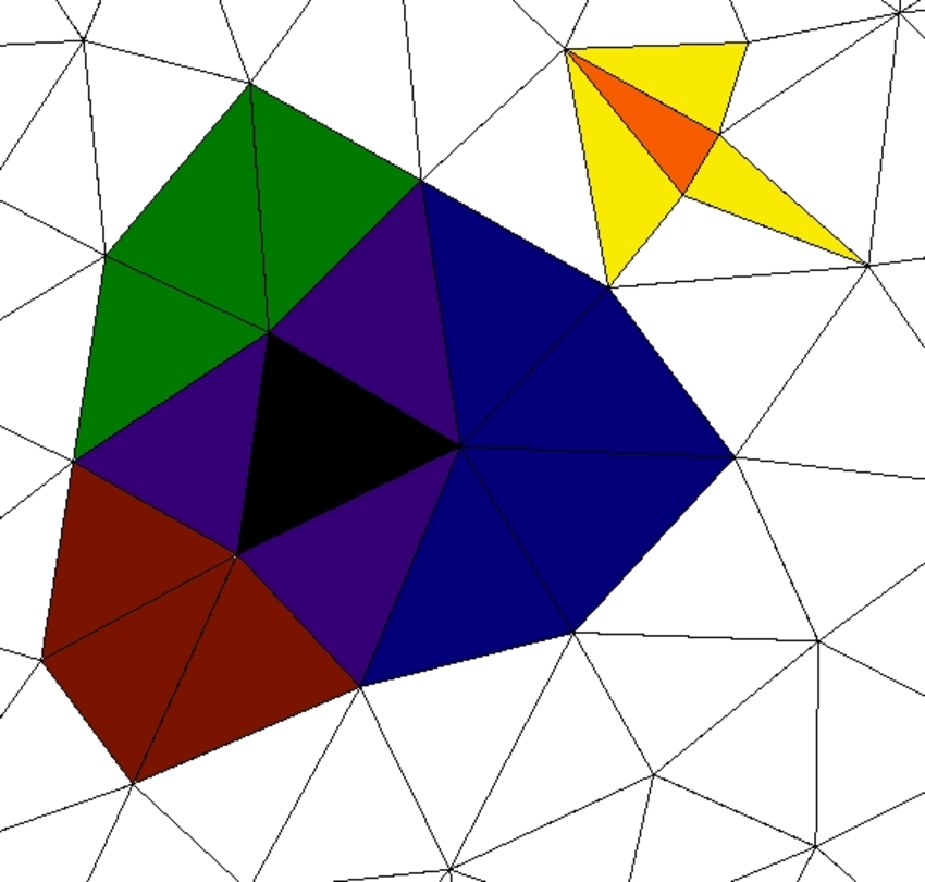
We now formally construct the generalized vertex-based slope limiter based off the Barth–Jespersen limiter [25, 6]. In this context we define a neighborhood as comprised of those elements that share a common vertex 𝒙isubscript𝒙𝑖\boldsymbol{x}_{i}, indexed with respect to every vertex of each finite element cell ΩejsubscriptΩsubscript𝑒𝑗\Omega_{e_{j}}. More clearly, we define the focal neighborhood Ωf={Ωej}isubscriptÎ©đ‘“subscriptsubscriptΩsubscript𝑒𝑗𝑖\Omega_{f}=\{\Omega_{e_{j}}\}_{i} (in the sense of the foci of geometric optics, as shown in Figure 2) as the collection of elements such that 𝒙i∈Ωejsubscript𝒙𝑖subscriptΩsubscript𝑒𝑗\boldsymbol{x}_{i}\in\Omega_{e_{j}} — where {Ωej}isubscriptsubscriptΩsubscript𝑒𝑗𝑖\{\Omega_{e_{j}}\}_{i} includes the base element ΩeisubscriptΩsubscript𝑒𝑖\Omega_{e_{i}} — such that i=1,2,3𝑖123i=1,2,3 over triangular elements.

We now note that one must choose a base space in which to implement this slope limiter (e.g. the physical ΩΩ\Omega or master ℳℳ\mathcal{M} element spaces, etc.). A fairly common choice (viz. [28, 25]) is to limit with respect to the full physical space ΩΩ\Omega. However, in the context of the local DG formulation this choice is not always so clearly taken. That is, given our transformations from §3.1, it is clear that we may not require the full Dubiner–Taylor transform ℒℒ\mathcal{L} but rather have the option to restrict to the master element space ℳℳ\mathcal{M} by simply using the invertible map 𝐍𝐍\mathbf{N}. More clearly, since local DG formulations often exploit computational efficiency by working over a master element representation ℳℳ\mathcal{M}, we are presented with a choice of composition maps to limit in the master or physical element spaces as shown in Figure 1, and given either by 𝐍−1∘ℒℳ∘𝐍superscript𝐍1subscriptℒℳ𝐍\mathbf{N}^{-1}\circ\mathscr{L}_{\mathcal{M}}\circ\mathbf{N} over ℳℳ\mathcal{M}, or by ℒ−1∘ℒΩ∘ℒsuperscriptℒ1subscriptℒΩℒ\mathcal{L}^{-1}\circ\mathscr{L}_{\Omega}\circ\mathcal{L} over ΩΩ\Omega. However, since (3.15) shows that ℒℒ\mathcal{L} requires the extra algorithmic step of transforming back into the physical coordinate frame ΩΩ\Omega, in the name of computational efficiency, we clearly prefer the former composition given the context of a relatively standard local DG method. However, when working in a global DG formulation where one elects, for example, a global linear solve, it may be more beneficial to limit with respect to ΩΩ\Omega, which as shown in Figure 1 may also be easily accomplished.

Now, we may define the explicit role of the vertex slope limiter as: a method of finding the limiter matrix đœ¶=(đœ¶1,
,đœ¶m)Tđœ¶superscriptsubscriptđœ¶1
subscriptđœ¶đ‘šđ‘‡\boldsymbol{\alpha}=(\boldsymbol{\alpha}_{1},\ldots,\boldsymbol{\alpha}_{m})^{T} such that for the solution vector satisfying đ‘Œh=(U1,
,Um)Tsubscriptđ‘Œâ„Žsuperscriptsubscript𝑈1
subscript𝑈𝑚𝑇\boldsymbol{U}_{h}=(U_{1},\ldots,U_{m})^{T}, with m𝑚m the number of unknowns in the system of equations, a vector defined by đœ¶=(α(0),
,α(k))Tđœ¶superscriptsuperscriptđ›Œ0
superscriptđ›Œđ‘˜đ‘‡\boldsymbol{\alpha}=(\alpha^{(0)},\ldots,\alpha^{(k)})^{T} for each order derivative i+j≀k𝑖𝑗𝑘i+j\leq k, the limiter coefficients α(i+j)∈[0,1]superscriptđ›Œđ‘–đ‘—01\alpha^{(i+j)}\in[0,1] allow for a recasting of the renormalized solution in (3.6) componentwise in the vertex slope limited form with respect to a focal stencil, that is Ωfi⊂ΩfsubscriptΩsubscript𝑓𝑖subscriptÎ©đ‘“\Omega_{f_{i}}\subset\Omega_{f} for a fixed vertex 𝒙isubscript𝒙𝑖\boldsymbol{x}_{i} (see Figure 4 for more detail).

Refer to caption
Figure 2: Here we show the focal neighborhood ΩfsubscriptÎ©đ‘“\Omega_{f} of a base element ΩeisubscriptΩsubscript𝑒𝑖\Omega_{e_{i}} filled in black. Green, red and blue are the three focal neighborhood groups based at vertices 𝒙isubscript𝒙𝑖\boldsymbol{x}_{i} of the black base cell, while purple are cells contained in more than one of the two focal neighbor stencils (incidentally comprising the edge neighborhoood of ΩeisubscriptΩsubscript𝑒𝑖\Omega_{e_{i}}). In a contrasting geometric locale, the orange base cell’s edge neighbors ΩEjsubscriptΩsubscript𝐾𝑗\Omega_{E_{j}} are each filled in yellow, comprising the edge neighborhood ΩEsubscriptÎ©đž\Omega_{E}. See Figure 4 for details.

In fact, regardless of the initial location containing the state vector (i.e. with respect to ℳℳ\mathcal{M} or with respect to ΩΩ\Omega) by simply using our transformations 𝐒𝐒\mathbf{S} and 𝐍𝐍\mathbf{N} from §2 we can recast (3.6) in the master element space ℳℳ\mathcal{M} such that componentwise we have the vertex slope limited approximate solution Uvsuperscript𝑈vU^{\mathrm{v}} which satisfies:

Uv=UÂŻâ€‹Ï‚00+∑0<i+j≀kα(i+j)​ςi​j​(∂i+jU∂Οi​∂ηj)|c,superscript𝑈v¯𝑈subscript𝜍00evaluated-atsubscript0𝑖𝑗𝑘superscriptđ›Œđ‘–đ‘—subscript𝜍𝑖𝑗superscript𝑖𝑗𝑈superscript𝜉𝑖superscript𝜂𝑗𝑐U^{\mathrm{v}}=\bar{U}\varsigma_{00}+\sum_{0<i+j\leq k}\alpha^{(i+j)}\varsigma_{ij}\left(\frac{\partial^{i+j}U}{\partial\xi^{i}\partial\eta^{j}}\right)\bigg{|}_{c}, (3.16)

where U¯¯𝑈\bar{U} and U𝑈U correspond to the approximate solution vector đ‘Œhsubscriptđ‘Œâ„Ž\boldsymbol{U}_{h} transformed to the master element frame in the Taylor basis representation.

Now, notice that above there exists only one α(i+j)superscriptđ›Œđ‘–đ‘—\alpha^{(i+j)} for each top k𝑘k–th order mixed derivative in ÎŸđœ‰\xi and Î·đœ‚\eta. In order to recover the α(i+j)superscriptđ›Œđ‘–đ‘—\alpha^{(i+j)}’s in the polynomial basis expansion, we must decompose our solution Taylor expansion into mixed order linear reconstructions. To do this, we first order our Taylor polynomial into a hierarchical basis such that each monomial index b=b​(i,j)𝑏𝑏𝑖𝑗b=b(i,j) is provided using the lexicographic ordering with ordered lattice pairs (i,j)𝑖𝑗(i,j) given by the sequence (0,0)<(0,1)<(1,0)<(0,2)<(1,1)<
=(i,j)0001100211
𝑖𝑗(0,0)<(0,1)<(1,0)<(0,2)<(1,1)<\ldots=(i,j) corresponding to indices b𝑏b, respectively; that is by the sequence (1)<(2)<(3)<(4)<(5)<
<(b)​
<(s)12345
𝑏
𝑠(1)<(2)<(3)<(4)<(5)<\ldots<(b)\ldots<(s) in the Taylor expansion. In fact, the monomial index in the hierarchy may be determined by the diophantine equation:

b=j2​(j+1)+i​j+i2​(i+3)+1.𝑏𝑗2𝑗1𝑖𝑗𝑖2𝑖31b=\frac{j}{2}\left(j+1\right)+ij+\frac{i}{2}\left(i+3\right)+1. (3.17)

Then we generate the hierarchical triangular sequence s=s​(p)𝑠𝑠𝑝s=s(p), where p=p​(i,j)𝑝𝑝𝑖𝑗p=p(i,j) satisfies p=(i+j)𝑝𝑖𝑗p=(i+j), such that s𝑠s determines the upper bound on the degrees of freedom in the polynomial expansion,

s=12​(p+1)​(p+2),given​inverse​g=g​(s)​such​that​g=⌊12+2​s⌋,formulae-sequence𝑠12𝑝1𝑝2giveninverse𝑔𝑔𝑠suchthat𝑔122𝑠s=\frac{1}{2}(p+1)(p+2),\quad\mathrm{given\ inverse}\ g=g(s)\ \mathrm{such\ that}\ g=\bigg{\lfloor}\frac{1}{2}+\sqrt{2s}\bigg{\rfloor}, (3.18)

where ⌊⋅⌋⋅\lfloor\cdot\rfloor is the usual floor function. Note that in particular we may use g=g​(s)𝑔𝑔𝑠g=g(s) or g=g​(b)𝑔𝑔𝑏g=g(b) for g​(b)âˆˆđ”©đ‘”đ‘đ”©g(b)\in\mathfrak{l} corresponding to level đ”©â‰ đ”©t​o​pđ”©subscriptđ”©đ‘Ąđ‘œđ‘\mathfrak{l}\neq\mathfrak{l}_{top} (defined below) since by virtue of the mapping (3.18) both return the same value.

(Ο1,η1)subscript𝜉1subscript𝜂1(\xi_{1},\eta_{1})(Ο3,η3)subscript𝜉3subscript𝜂3(\xi_{3},\eta_{3})(Ο2,η2)subscript𝜉2subscript𝜂2(\xi_{2},\eta_{2})ΩelsubscriptΩsubscript𝑒𝑙\Omega_{e_{l}}Base element, ΩelâˆˆÎ©đ”›isubscriptΩsubscript𝑒𝑙subscriptΩsubscript𝔛𝑖\Omega_{e_{l}}\in\Omega_{\mathfrak{X}_{i}}(Οc,ηc)subscript𝜉𝑐subscript𝜂𝑐(\xi_{c},\eta_{c})A schematic of the vertex-based methodsCentroid of ΩelâˆˆÎ©đ”›isubscriptΩsubscript𝑒𝑙subscriptΩsubscript𝔛𝑖\Omega_{e_{l}}\in\Omega_{\mathfrak{X}_{i}}∙i∙𝑖\bullet\ \ i– the first index of the Taylor expansion∙j∙𝑗\bullet\ \ j– the second index of the Taylor expansion∙b​(i,j)∙𝑏𝑖𝑗\bullet\ \ b(i,j)– the monomial index∙𝒞b∙subscript𝒞𝑏\bullet\ \ \mathscr{C}_{b}– the Taylor monomial of index b𝑏b∙Ub,i(i+j)∙superscriptsubscript𝑈𝑏𝑖𝑖𝑗\bullet\ \ U_{b,i}^{(i+j)}– the linear reconstruction at (Οi,ηi)subscript𝜉𝑖subscript𝜂𝑖(\xi_{i},\eta_{i})∙Ui,bmax,Ui,bmin∙superscriptsubscript𝑈𝑖𝑏superscriptsubscript𝑈𝑖𝑏\bullet\ \ U_{i,b}^{\max},U_{i,b}^{\min}– the extrema over the stencilÎ©đ”›isubscriptΩsubscript𝔛𝑖\Omega_{\mathfrak{X}_{i}}∙α(q)∙superscriptđ›Œđ‘ž\bullet\ \ \alpha^{(q)}– the limiting coefficients on ΩelsubscriptΩsubscript𝑒𝑙\Omega_{e_{l}}
Figure 3: Here we provide a key for the vertex and Barth–Jespersen limiters of §3.2–§3.2.1. Generally theses limiting procedures depend on the chosen stencil Î©đ”›isubscriptΩsubscript𝔛𝑖\Omega_{\mathfrak{X}_{i}} and a local linear reconstruction of the solution in order to develop the limiting coefficients from (3.16).

Then letting Ui,c,bejsubscriptsuperscript𝑈subscript𝑒𝑗𝑖𝑐𝑏U^{e_{j}}_{i,c,b} be the value of the b𝑏b-th term in the polynomial basis of đ‘Œhsubscriptđ‘Œâ„Ž\boldsymbol{U}_{h} at the centroid c𝑐c of element Ω^ejsubscript^Ωsubscript𝑒𝑗\hat{\Omega}_{e_{j}} containing 𝒙i=(Οi,ηi)subscript𝒙𝑖subscript𝜉𝑖subscript𝜂𝑖\boldsymbol{x}_{i}=(\xi_{i},\eta_{i}) in the master element representation, we define the maximum Ui,bmaxsuperscriptsubscript𝑈𝑖𝑏U_{i,b}^{\max} and minimum Ui,bminsuperscriptsubscript𝑈𝑖𝑏U_{i,b}^{\min} values for each unknown monomial at 𝒙isubscript𝒙𝑖\boldsymbol{x}_{i} over the focal stencil ΩfisubscriptΩsubscript𝑓𝑖\Omega_{f_{i}} situated with respect to the master element frame Ω^fisubscript^Ωsubscript𝑓𝑖\hat{\Omega}_{f_{i}} as

Ui,bmax=maxΩ^ej∈Ω^fi⁥{Ui,b,cej}andUi,bmin=minΩ^ej∈Ω^fi⁥{Ui,b,cej}.formulae-sequencesuperscriptsubscript𝑈𝑖𝑏subscriptsubscript^Ωsubscript𝑒𝑗subscript^Ωsubscript𝑓𝑖subscriptsuperscript𝑈subscript𝑒𝑗𝑖𝑏𝑐andsuperscriptsubscript𝑈𝑖𝑏subscriptsubscript^Ωsubscript𝑒𝑗subscript^Ωsubscript𝑓𝑖subscriptsuperscript𝑈subscript𝑒𝑗𝑖𝑏𝑐U_{i,b}^{\max}=\max_{\hat{\Omega}_{{e}_{j}}\in\hat{\Omega}_{f_{i}}}\big{\{}U^{e_{j}}_{i,b,c}\big{\}}\quad\mathrm{and}\quad U_{i,b}^{\min}=\min_{\hat{\Omega}_{{e}_{j}}\in\hat{\Omega}_{f_{i}}}\big{\{}U^{e_{j}}_{i,b,c}\big{\}}. (3.19)

Now, we are able to define the (i+j)𝑖𝑗(i+j)-th linear reconstructions Ub,i(i+j)superscriptsubscript𝑈𝑏𝑖𝑖𝑗U_{b,i}^{(i+j)} over the vertices 𝒙isubscript𝒙𝑖\boldsymbol{x}_{i} of any element by taking derivations with respect to the monomial coefficients of (3.16). That is, the linear perturbation of the constant term is constructed such that,

Ub,i(1)=UÂŻ+∂Ui∂Ο|c​(Οi−Οc)+∂Ui∂η|c​(ηi−ηc),for​s=3.formulae-sequencesuperscriptsubscript𝑈𝑏𝑖1¯𝑈evaluated-atsubscript𝑈𝑖𝜉𝑐subscript𝜉𝑖subscript𝜉𝑐evaluated-atsubscript𝑈𝑖𝜂𝑐subscript𝜂𝑖subscript𝜂𝑐for𝑠3U_{b,i}^{(1)}=\bar{U}+\frac{\partial U_{i}}{\partial\xi}\bigg{|}_{c}(\xi_{i}-\xi_{c})+\frac{\partial U_{i}}{\partial\eta}\bigg{|}_{c}(\eta_{i}-\eta_{c}),\qquad\mathrm{for}\ s=3. (3.20)

Moreover, it is now direct to construct the higher order terms whereby setting

𝒞b=(∂i+jU∂Οi​∂ηj)|cforb​(i,j)>1,formulae-sequencesubscript𝒞𝑏evaluated-atsuperscript𝑖𝑗𝑈superscript𝜉𝑖superscript𝜂𝑗𝑐for𝑏𝑖𝑗1\mathscr{C}_{b}=\left(\frac{\partial^{i+j}U}{\partial\xi^{i}\partial\eta^{j}}\right)\bigg{|}_{c}\quad\mathrm{for}\ \ b(i,j)>1,

such that for any mixed derivative order in the hierarchical basis — as a property of the lexicographic ordering — we can write:

Ub,i(i+j)=𝒞b+𝒞b+g​(ηi−ηc)+𝒞b+g+1​(Οi−Οc),superscriptsubscript𝑈𝑏𝑖𝑖𝑗subscript𝒞𝑏subscript𝒞𝑏𝑔subscript𝜂𝑖subscript𝜂𝑐subscript𝒞𝑏𝑔1subscript𝜉𝑖subscript𝜉𝑐U_{b,i}^{(i+j)}=\mathscr{C}_{b}+\mathscr{C}_{b+g}(\eta_{i}-\eta_{c})+\mathscr{C}_{b+g+1}(\xi_{i}-\xi_{c}), (3.21)

for any polynomial order k𝑘k. Proceeding, we can now define the correction factors αb(i+j)superscriptsubscriptđ›Œđ‘đ‘–đ‘—\alpha_{b}^{(i+j)} for each element ΩelsubscriptΩsubscript𝑒𝑙\Omega_{e_{l}}, where the vertex-based condition is simply defined as

αb(i+j)=min𝒙i∈Ω^el⁥{min⁥{1,(Ui,bmax−Ui,c,belUb,i(i+j)−Ui,c,bel)},forUb,i(i+j)>Ui,c,bel1,forUb,i(i+j)=Ui,c,belmin⁥{1,(Ui,bmin−Ui,c,belUb,i(i+j)−Ui,c,bel)},forUb,i(i+j)<Ui,c,belsuperscriptsubscriptđ›Œđ‘đ‘–đ‘—subscriptsubscript𝒙𝑖subscript^Ωsubscript𝑒𝑙cases1superscriptsubscript𝑈𝑖𝑏subscriptsuperscript𝑈subscript𝑒𝑙𝑖𝑐𝑏superscriptsubscript𝑈𝑏𝑖𝑖𝑗superscriptsubscript𝑈𝑖𝑐𝑏subscript𝑒𝑙forsuperscriptsubscript𝑈𝑏𝑖𝑖𝑗subscriptsuperscript𝑈subscript𝑒𝑙𝑖𝑐𝑏1forsuperscriptsubscript𝑈𝑏𝑖𝑖𝑗subscriptsuperscript𝑈subscript𝑒𝑙𝑖𝑐𝑏1superscriptsubscript𝑈𝑖𝑏subscriptsuperscript𝑈subscript𝑒𝑙𝑖𝑐𝑏superscriptsubscript𝑈𝑏𝑖𝑖𝑗superscriptsubscript𝑈𝑖𝑐𝑏subscript𝑒𝑙forsuperscriptsubscript𝑈𝑏𝑖𝑖𝑗subscriptsuperscript𝑈subscript𝑒𝑙𝑖𝑐𝑏\alpha_{b}^{(i+j)}=\min_{\boldsymbol{x}_{i}\in\hat{\Omega}_{e_{l}}}\begin{cases}\min\Bigg{\{}1,\left(\frac{U_{i,b}^{\max}-U^{e_{l}}_{i,c,b}}{U_{b,i}^{(i+j)}-U_{i,c,b}^{e_{l}}}\right)\Bigg{\}},&\mathrm{for}\ \ U_{b,i}^{(i+j)}>U^{e_{l}}_{i,c,b}\\ \qquad 1,&\mathrm{for}\ \ U_{b,i}^{(i+j)}=U^{e_{l}}_{i,c,b}\\ \min\Bigg{\{}1,\left(\frac{U_{i,b}^{\min}-U^{e_{l}}_{i,c,b}}{U_{b,i}^{(i+j)}-U_{i,c,b}^{e_{l}}}\right)\Bigg{\}},&\mathrm{for}\ \ U_{b,i}^{(i+j)}<U^{e_{l}}_{i,c,b}\end{cases} (3.22)

which, again, is determined separately for each monomial represented in the master frame.
Refer to caption
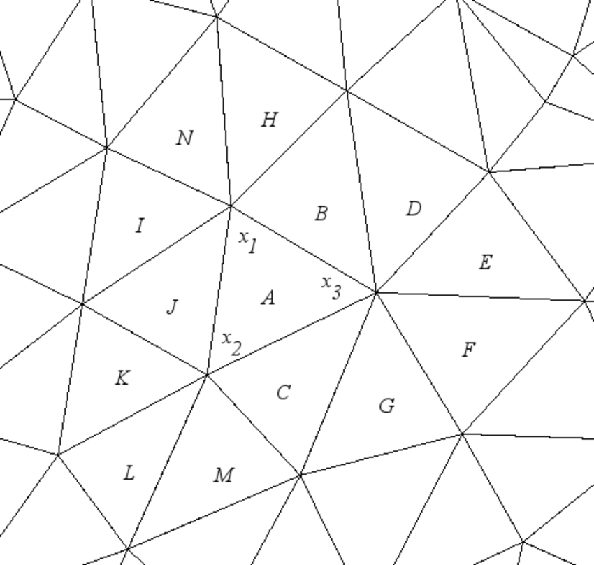
Figure 4: Here we show the focal stencil ΩfisubscriptΩsubscript𝑓𝑖\Omega_{f_{i}} and the edge stencil ΩEisubscriptΩsubscript𝐾𝑖\Omega_{E_{i}} of a base element Ωel=AsubscriptΩsubscript𝑒𝑙𝐮\Omega_{e_{l}}=A. The stencils are defined with respect to the base elements vertices 𝒙isubscript𝒙𝑖\boldsymbol{x}_{i} for i=1,2,3𝑖123i=1,2,3, such that the focal stencil at 𝒙1subscript𝒙1\boldsymbol{x}_{1} is Ωf1={J,I,N,H,B,A}subscriptΩsubscript𝑓1đœđŒđ‘đ»đ”đŽ\Omega_{f_{1}}=\{J,I,N,H,B,A\}, and likewise Ωf2={J,K,L,M,C,A}subscriptΩsubscript𝑓2đœđŸđżđ‘€đ¶đŽ\Omega_{f_{2}}=\{J,K,L,M,C,A\} and Ωf3={C,G,F,E,D,B,A}subscriptΩsubscript𝑓3đ¶đșđčđžđ·đ”đŽ\Omega_{f_{3}}=\{C,G,F,E,D,B,A\}. Similarly the edge stencils are given by: ΩE1={J,B,A}subscriptΩsubscript𝐾1đœđ”đŽ\Omega_{E_{1}}=\{J,B,A\}, ΩE2={J,C,A}subscriptΩsubscript𝐾2đœđ¶đŽ\Omega_{E_{2}}=\{J,C,A\} and ΩE3={B,C,A}subscriptΩsubscript𝐾3đ”đ¶đŽ\Omega_{E_{3}}=\{B,C,A\}. Notice that the union of sets recovers the focal neighborhood (Ωf=âˆȘiΩfisubscriptÎ©đ‘“subscript𝑖subscriptΩsubscript𝑓𝑖\Omega_{f}=\cup_{i}\Omega_{f_{i}}) and the edge neighborhood (ΩE=âˆȘiΩEisubscriptÎ©đžsubscript𝑖subscriptΩsubscript𝐾𝑖\Omega_{E}=\cup_{i}\Omega_{E_{i}}), while the restriction of the symmetric difference of sets defines the focal neighborhood group (⊖iΩfi|Ωfjsubscriptsymmetric-difference𝑖evaluated-atsubscriptΩsubscript𝑓𝑖subscriptΩsubscript𝑓𝑗\ominus_{i}\Omega_{f_{i}}|_{\Omega_{f_{j}}}) and edge neighborhood group (⊖iΩEi|ΩEjsubscriptsymmetric-difference𝑖evaluated-atsubscriptΩsubscript𝐾𝑖subscriptΩsubscript𝐾𝑗\ominus_{i}\Omega_{E_{i}}|_{\Omega_{E_{j}}}) for any vertex j𝑗j.

These αb(i+j)superscriptsubscriptđ›Œđ‘đ‘–đ‘—\alpha_{b}^{(i+j)} determine a set of limiting constraints for every hierarchical monomial in the Taylor expansion, but as in [25], we minimize over derivatives of similar top order, such that we recover the components:

Î±đ”©â€‹(p)(i+j)=ming​(b)=đ”©â€‹(p0)⁥αb(i+j).superscriptsubscriptđ›Œđ”©đ‘đ‘–đ‘—subscriptđ‘”đ‘đ”©subscript𝑝0superscriptsubscriptđ›Œđ‘đ‘–đ‘—\alpha_{\mathfrak{l}(p)}^{(i+j)}=\min_{g(b)=\mathfrak{l}(p_{0})}\alpha_{b}^{(i+j)}. (3.23)

Notice that these limiting coefficients span the level đ”©â€‹(p0)đ”©subscript𝑝0\mathfrak{l}(p_{0}), not the hierarchical index b𝑏b corresponding to level đ”©â€‹(p)đ”©đ‘\mathfrak{l}(p) (where p𝑝p and p0subscript𝑝0p_{0} are fully explained below). That is, in the hierarchical basis the linear reconstructions from the perturbation at the level below (i.e. level (đ”©âˆ’1)đ”©1(\mathfrak{l}-1)) are what effectively determine the limiting coefficient at level đ”©đ”©\mathfrak{l} (e.g. the gradient terms). More precisely, the level đ”©=đ”©â€‹(p0)đ”©đ”©subscript𝑝0\mathfrak{l}=\mathfrak{l}(p_{0}) is determined with respect to the sequence of integers starting at p0​(p0−1)/2+1subscript𝑝0subscript𝑝0121p_{0}(p_{0}-1)/2+1 and increasing by one until reaching p0​(p0+1)/2subscript𝑝0subscript𝑝012p_{0}(p_{0}+1)/2. Then the level is defined by đ”©=sup{g​(p0​(p0−1)/2+1),
,g​(p0​(p0+1)/2)}đ”©supremum𝑔subscript𝑝0subscript𝑝0121
𝑔subscript𝑝0subscript𝑝012\mathfrak{l}=\sup\{g(p_{0}(p_{0}-1)/2+1),\ldots,g(p_{0}(p_{0}+1)/2)\}, where p0=1subscript𝑝01p_{0}=1 for the strictly linear case, and in general is a positive integer such that p0≀psubscript𝑝0𝑝p_{0}\leq p and is fully determined by g​(b​(i,j))𝑔𝑏𝑖𝑗g(b(i,j)). In general however, the level đ”©â€‹(p)đ”©đ‘\mathfrak{l}(p) spans đ”©=sup{g​(p​(p+1)/2)+1,
,g​((p+1)​(p+2)/2)}đ”©supremum𝑔𝑝𝑝121
𝑔𝑝1𝑝22\mathfrak{l}=\sup\{g(p(p+1)/2)+1,\ldots,g((p+1)(p+2)/2)\} such that the level below đ”©â€‹(p0)đ”©subscript𝑝0\mathfrak{l}(p_{0}) simply corresponds to setting p=p0−1𝑝subscript𝑝01p=p_{0}-1.

Finally we limit the magnitude of the correction by the maximum value of every correction factor of greater than or equal order. In other words, we do not allow a higher order correction to demonstrate greater regularity than a lower order correction, and in fact empirical experimentation has found this to be a necessary constraint. That is, setting q=(i+j)𝑞𝑖𝑗q=(i+j) and r=(iâ€Č+jâ€Č)𝑟superscript𝑖â€Čsuperscript𝑗â€Čr=(i^{\prime}+j^{\prime}) for iâ€Čsuperscript𝑖â€Či^{\prime} and jâ€Čsuperscript𝑗â€Čj^{\prime} indices, then we determine an upper bound on the correction parameter by resetting:

α(q):=maxq≀r,đ”©â‰€đ”©topâĄÎ±đ”©(r),∀q≄1,∀r≄q.formulae-sequenceassignsuperscriptđ›Œđ‘žsubscriptformulae-sequenceđ‘žđ‘Ÿđ”©subscriptđ”©topsuperscriptsubscriptđ›Œđ”©đ‘Ÿformulae-sequencefor-all𝑞1for-all𝑟𝑞\alpha^{(q)}:=\max_{q\leq r,\mathfrak{l}\leq\mathfrak{l}_{\mathrm{top}}}\alpha_{\mathfrak{l}}^{(r)},\quad\forall q\geq 1,\ \forall r\geq q. (3.24)

The top level đ”©topsubscriptđ”©top\mathfrak{l}_{\mathrm{top}} simply corresponds to the level whose upper bound is determined by g​(s)=g​(b)𝑔𝑠𝑔𝑏g(s)=g(b). Also notice that the derivative order (i+j)𝑖𝑗(i+j) is fundamentally coupled to the level đ”©đ”©\mathfrak{l}, and so is in some ways redundant notation which we have used in order to emphasize this coupling.

It is also worth noting, that as a consequence of the above construction we are now easily able to implement an arbitrarily higher-order extension of the Barth–Jespersen limiter [25, 6], where we may perform the exact steps as above, but simply exchange (3.19) with

Ui,bmax=maxΩ^ej∈Ω^Ei⁥{Ui,b,cej}andUi,bmin=minΩ^ej∈Ω^Ei⁥{Ui,b,cej},formulae-sequencesuperscriptsubscript𝑈𝑖𝑏subscriptsubscript^Ωsubscript𝑒𝑗subscript^Ωsubscript𝐾𝑖subscriptsuperscript𝑈subscript𝑒𝑗𝑖𝑏𝑐andsuperscriptsubscript𝑈𝑖𝑏subscriptsubscript^Ωsubscript𝑒𝑗subscript^Ωsubscript𝐾𝑖subscriptsuperscript𝑈subscript𝑒𝑗𝑖𝑏𝑐U_{i,b}^{\max}=\max_{\hat{\Omega}_{{e}_{j}}\in\hat{\Omega}_{E_{i}}}\big{\{}U^{e_{j}}_{i,b,c}\big{\}}\quad\mathrm{and}\quad U_{i,b}^{\min}=\min_{\hat{\Omega}_{{e}_{j}}\in\hat{\Omega}_{E_{i}}}\big{\{}U^{e_{j}}_{i,b,c}\big{\}}, (3.25)

where Ω^Eisubscript^Ωsubscript𝐾𝑖\hat{\Omega}_{E_{i}} is the edge stencil of Ω^ejsubscript^Ωsubscript𝑒𝑗\hat{\Omega}_{e_{j}} at 𝒙isubscript𝒙𝑖\boldsymbol{x}_{i} in the master element representation — or the corresponding set of those physical elements sharing an edge with ΩejsubscriptΩsubscript𝑒𝑗\Omega_{e_{j}} at vertex 𝒙isubscript𝒙𝑖\boldsymbol{x}_{i} such that the base element Ωej∈ΩEisubscriptΩsubscript𝑒𝑗subscriptΩsubscript𝐾𝑖\Omega_{e_{j}}\in\Omega_{E_{i}} (see Figure 2).

A schematic is provided in Figure 3 which is meant to simplify the notation and unify the basic principles underlying both the vertex and Barth–Jespersen limiters (as well as the adapted vertex-based limiters of §3.2.1).

3.2.1 §​3.2​a§3.2𝑎\S 3.2a On adapted vertex based limiters

Both the vertex limiter and the Barth–Jespersen limiter from §3.2 demonstrate a similar — though often times non-ideal — behavior. That is, notice that in both the definition of (3.19) and 3.25) that we have found a maximum or minimum with respect to a local neighborhood of the mesh. Hence, in either case, when we compute the limiting coefficients in (3.22) a local bound (e.g. (3.25)) is always achieved, even in the degenerate case of when Ui,bmin=Ui,bmaxsuperscriptsubscript𝑈𝑖𝑏superscriptsubscript𝑈𝑖𝑏U_{i,b}^{\min}=U_{i,b}^{\max}.

As a consequence of this, the numerator in the quotients of (3.22) vanish on elements admitting a local extremum, leading to persistent and excessive diffusivity (i.e. limiting α=0đ›Œ0\alpha=0 at each such timestep) arising at all orders in each local extrema of the mesh, even when those extrema are neither spurious nor potentially unstable; and moreover, this behavior compounds in p𝑝p since as p𝑝p increases the number of degrees of freedom (i.e. monomials) in the solution which have local extrema also increases nonlinearly.

This behavior over values of local extrema can become quite dominant depending on the mesh geometry. In particular, since the vertex-based limiter has a larger local neighborhood (i.e. the focal neighborhood) than the Barth–Jespersen limiter, in principle it should provide more information from which to glean a more accurate approximate local reconstruction. However, due to this “diffusivity,” the larger local neighborhood actually lends itself towards increasing the nonlocality of the diffusive effects of the neighborhood-wise extrema as p↗pmax↗𝑝subscript𝑝p\nearrow p_{\max}, and hence in practice can actually precipitate greater diffusion in the vertex limiter than the native Barth–Jespersen limiter as p𝑝p increases (up to the mesh geometry).

In order to reduce this so-called “blind diffusion” in both limiters we introduce a simple functional which attempts to treat a portion of this special case separately. That is, we simply replace (3.22) with:

αb(i+j)=min𝒙i∈Ωel⁥{min⁥{1,(Ui,bmax−Ui,c,belUb,i(i+j)−Ui,c,bel)},forUb,i(i+j)>Ui,c,belmin⁥{fmax,|Ui,bmax−Ui,bminUb,i(i+j)−Ui,c,bel|},forUi,c,bel=Ui,bmax1,forUb,i(i+j)=Ui,c,belmin⁥{fmin,|Ui,bmin−Ui,bmaxUb,i(i+j)−Ui,c,bel|},forUi,c,bel=Ui,bminmin⁥{1,(Ui,bmin−Ui,c,belUb,i(i+j)−Ui,c,bel)},forUb,i(i+j)<Ui,c,belsuperscriptsubscriptđ›Œđ‘đ‘–đ‘—subscriptsubscript𝒙𝑖subscriptΩsubscript𝑒𝑙cases1superscriptsubscript𝑈𝑖𝑏subscriptsuperscript𝑈subscript𝑒𝑙𝑖𝑐𝑏superscriptsubscript𝑈𝑏𝑖𝑖𝑗superscriptsubscript𝑈𝑖𝑐𝑏subscript𝑒𝑙forsuperscriptsubscript𝑈𝑏𝑖𝑖𝑗subscriptsuperscript𝑈subscript𝑒𝑙𝑖𝑐𝑏subscript𝑓superscriptsubscript𝑈𝑖𝑏superscriptsubscript𝑈𝑖𝑏superscriptsubscript𝑈𝑏𝑖𝑖𝑗superscriptsubscript𝑈𝑖𝑐𝑏subscript𝑒𝑙forsubscriptsuperscript𝑈subscript𝑒𝑙𝑖𝑐𝑏superscriptsubscript𝑈𝑖𝑏1forsuperscriptsubscript𝑈𝑏𝑖𝑖𝑗subscriptsuperscript𝑈subscript𝑒𝑙𝑖𝑐𝑏subscript𝑓superscriptsubscript𝑈𝑖𝑏superscriptsubscript𝑈𝑖𝑏superscriptsubscript𝑈𝑏𝑖𝑖𝑗superscriptsubscript𝑈𝑖𝑐𝑏subscript𝑒𝑙forsubscriptsuperscript𝑈subscript𝑒𝑙𝑖𝑐𝑏superscriptsubscript𝑈𝑖𝑏1superscriptsubscript𝑈𝑖𝑏subscriptsuperscript𝑈subscript𝑒𝑙𝑖𝑐𝑏superscriptsubscript𝑈𝑏𝑖𝑖𝑗superscriptsubscript𝑈𝑖𝑐𝑏subscript𝑒𝑙forsuperscriptsubscript𝑈𝑏𝑖𝑖𝑗subscriptsuperscript𝑈subscript𝑒𝑙𝑖𝑐𝑏\alpha_{b}^{(i+j)}=\min_{\boldsymbol{x}_{i}\in\Omega_{e_{l}}}\begin{cases}\ \min\Bigg{\{}1,\left(\frac{U_{i,b}^{\max}-U^{e_{l}}_{i,c,b}}{U_{b,i}^{(i+j)}-U_{i,c,b}^{e_{l}}}\right)\Bigg{\}},&\mathrm{for}\ \ U_{b,i}^{(i+j)}>U^{e_{l}}_{i,c,b}\\ \min\Bigg{\{}f_{\max},\bigg{|}\frac{U_{i,b}^{\max}-U_{i,b}^{\min}}{U_{b,i}^{(i+j)}-U_{i,c,b}^{e_{l}}}\bigg{|}\Bigg{\}},&\mathrm{for}\ \ U^{e_{l}}_{i,c,b}=U_{i,b}^{\max}\\ \qquad\qquad\qquad 1,&\mathrm{for}\ \ U_{b,i}^{(i+j)}=U^{e_{l}}_{i,c,b}\\ \min\Bigg{\{}f_{\min},\bigg{|}\frac{U_{i,b}^{\min}-U_{i,b}^{\max}}{U_{b,i}^{(i+j)}-U_{i,c,b}^{e_{l}}}\bigg{|}\Bigg{\}},&\mathrm{for}\ \ U^{e_{l}}_{i,c,b}=U_{i,b}^{\min}\\ \ \min\Bigg{\{}1,\left(\frac{U_{i,b}^{\min}-U^{e_{l}}_{i,c,b}}{U_{b,i}^{(i+j)}-U_{i,c,b}^{e_{l}}}\right)\Bigg{\}},&\mathrm{for}\ \ U_{b,i}^{(i+j)}<U^{e_{l}}_{i,c,b}\end{cases} (3.26)

where fmax,fmin∈(0,1)subscript𝑓subscript𝑓01f_{\max},f_{\min}\in(0,1) are constants used to limit the rate at which the extrema diffuse (that is, reduce the rate at which error is introduced into the solution), and when fmax=fminsubscript𝑓subscript𝑓f_{\max}=f_{\min} we denote them by fdsubscript𝑓𝑑f_{d}.

We find when setting fd=1subscript𝑓𝑑1f_{d}=1 we generally get a very moderate improvement in the limiting error behavior of both the vertex and Barth–Jespersen limiters. Nevertheless, clearly (3.26) has only accounted partially for the degenerate local extrema cases, in particular it still fails to properly account for the case of Ub,imin=Ub,imaxsuperscriptsubscript𝑈𝑏𝑖superscriptsubscript𝑈𝑏𝑖U_{b,i}^{\min}=U_{b,i}^{\max}, and the absolute value is used to account for the fact that the signs have not been separately controlled. We have developed strategies for adopting fixes for these issues into the limiter, but in general find even the augmented regimes to still demonstrate substantially more diffuse behavior than the restricted regime presented in §3.4, and so will suppress any further comment on the subject at present, simply noting that it is possible to improve upon the basic behavior of the limiter in p𝑝p by developing selection strategies to deal with the many special cases which arise over solutions locally, and where alternatively one is often also able to improve the error behavior by tuning fmaxsubscript𝑓f_{\max} and fminsubscript𝑓f_{\min}.

It should be additionally noted here that in [25] a mass lumping strategy is implemented with respect to the triangular meshes in order to prevent the formation of undershoots and overshoots caused in the presence of the non-orthogonal Taylor mass matrix. It was also demonstrated in [25] that this strategy can have a measurably beneficial effect on the error behavior for p≀2𝑝2p\leq 2, and is thus clearly worth further examination at higher p𝑝p. We will return to this issue briefly in §4 as a note of comparison between the implementational strategies.

3.3 §​3.3§3.3\S 3.3 The hierarchical reconstruction via MUSCL or ENO

We now consider the hierarchical reconstruction scheme presented in [1] and [27]. Formally in this setting we simply take derivatives of (3.2) in the master element frame, and work locally over the averages and differences of these differential reconstructions. The method is presented as a two step process, where we start in step 1 at the highest order derivatives and work down to the lowest, with the caveat that the linear and constant terms are dealt with separately in step 2.

Step 1. Starting at the top order coefficient k𝑘k, a linearization of the (k−1)𝑘1(k-1)–st derivative of (3.2) is given by (3.21) in the Taylor basis for i+j=k−1𝑖𝑗𝑘1i+j=k-1. Here, however, we recover the entire higher order component including the nonlinear terms, so that we must employ our monomial index function b​(i,j)𝑏𝑖𝑗b(i,j) given in (3.17).

That is, beginning at the top level đ”©â€‹(k)đ”©đ‘˜\mathfrak{l}(k) for i+j=k𝑖𝑗𝑘i+j=k we define the linear part as satisfying:

UÂŻbl​i​n​e​a​r,Ωel(i+j):=𝒞b​(i,j),∀bâˆˆđ”©â€‹(k)∧∀ΩelâˆˆÎ©đ”›,formulae-sequenceassignsuperscriptsubscript¯𝑈subscript𝑏𝑙𝑖𝑛𝑒𝑎𝑟subscriptΩsubscript𝑒𝑙𝑖𝑗subscript𝒞𝑏𝑖𝑗for-allđ‘đ”©đ‘˜for-allsubscriptΩsubscript𝑒𝑙subscriptÎ©đ”›\bar{U}_{b_{linear},\Omega_{e_{l}}}^{(i+j)}:=\mathscr{C}_{b(i,j)},\quad\forall b\in\mathfrak{l}(k)\ \land\ \forall\Omega_{e_{l}}\in\Omega_{\mathfrak{X}}, (3.27)

where 𝔛𝔛\mathfrak{X} here and below may be f𝑓f or E𝐾E (i.e. the focal and the edge neighborhoods, respectively, as shown in both Figure 2 and Figure 4), and where here and below ∧\land is the logical conjunction operator and ∹\lor is the corresponding logical disjunction operator.

At the lower (nonlinear) levels (i.e. the levels đ”©đ”©\mathfrak{l} such that đ”©â€‹(1)<đ”©<đ”©â€‹(k)đ”©1đ”©đ”©đ‘˜\mathfrak{l}(1)<\mathfrak{l}<\mathfrak{l}(k)) by expansion – after recovering the i𝑖i and j𝑗j indices of the base b𝑏b–th component —then setting b~=b​(i+iâ€Č,j+jâ€Č)~𝑏𝑏𝑖superscript𝑖â€Č𝑗superscript𝑗â€Č\tilde{b}=b(i+i^{\prime},j+j^{\prime}) and integrating locally over each cell in the neighborhood, we have that:

UÂŻb,Ωel(i+j)=𝒞b​(i,j)+Ωel−1​∫Ωel{∑iâ€Č+jâ€Č>01iâ€Č!​jâ€Č!​𝒞b~​(η−ηc)iâ€Č​(Ο−Οc)jâ€Č}â€‹đ‘‘Î·â€‹đ‘‘ÎŸ,∀b~≀s∧∀ΩelâˆˆÎ©đ”›.formulae-sequencesuperscriptsubscript¯𝑈𝑏subscriptΩsubscript𝑒𝑙𝑖𝑗subscript𝒞𝑏𝑖𝑗superscriptsubscriptΩsubscript𝑒𝑙1subscriptsubscriptΩsubscript𝑒𝑙subscriptsuperscript𝑖â€Čsuperscript𝑗â€Č01superscript𝑖â€Čsuperscript𝑗â€Čsubscript𝒞~𝑏superscript𝜂subscript𝜂𝑐superscript𝑖â€Čsuperscript𝜉subscript𝜉𝑐superscript𝑗â€Čdifferential-d𝜂differential-d𝜉for-all~𝑏𝑠for-allsubscriptΩsubscript𝑒𝑙subscriptÎ©đ”›\bar{U}_{b,\Omega_{e_{l}}}^{(i+j)}=\mathscr{C}_{b(i,j)}+\Omega_{e_{l}}^{-1}\int_{\Omega_{e_{l}}}\bigg{\{}\sum_{i^{\prime}+j^{\prime}>0}\frac{1}{i^{\prime}!j^{\prime}!}\mathscr{C}_{\tilde{b}}(\eta-\eta_{c})^{i^{\prime}}(\xi-\xi_{c})^{j^{\prime}}\bigg{\}}d\eta d\xi,\quad\forall\tilde{b}\leq s\ \land\ \forall\Omega_{e_{l}}\in\Omega_{\mathfrak{X}}. (3.28)

Likewise for each level đ”©đ”©\mathfrak{l} we integrate the higher order perturbative terms such that:

UÂŻbs​l​o​p​e,Ωel(i+j)=Ωel−1​∫Ωel{∑iâ€Č+jâ€Č>01iâ€Č!​jâ€Č!​𝒞b~​(η−ηc)iâ€Č​(Ο−Οc)jâ€Č}â€‹đ‘‘Î·â€‹đ‘‘ÎŸ,∀b~≀s∧∀ΩelâˆˆÎ©đ”›.formulae-sequencesuperscriptsubscript¯𝑈subscript𝑏𝑠𝑙𝑜𝑝𝑒subscriptΩsubscript𝑒𝑙𝑖𝑗superscriptsubscriptΩsubscript𝑒𝑙1subscriptsubscriptΩsubscript𝑒𝑙subscriptsuperscript𝑖â€Čsuperscript𝑗â€Č01superscript𝑖â€Čsuperscript𝑗â€Čsubscript𝒞~𝑏superscript𝜂subscript𝜂𝑐superscript𝑖â€Čsuperscript𝜉subscript𝜉𝑐superscript𝑗â€Čdifferential-d𝜂differential-d𝜉for-all~𝑏𝑠for-allsubscriptΩsubscript𝑒𝑙subscriptÎ©đ”›\bar{U}_{b_{slope},\Omega_{e_{l}}}^{(i+j)}=\Omega_{e_{l}}^{-1}\int_{\Omega_{e_{l}}}\bigg{\{}\sum_{i^{\prime}+j^{\prime}>0}\frac{1}{i^{\prime}!j^{\prime}!}\mathscr{C}_{\tilde{b}}(\eta-\eta_{c})^{i^{\prime}}(\xi-\xi_{c})^{j^{\prime}}\bigg{\}}d\eta d\xi,\quad\forall\tilde{b}\leq s\ \land\ \forall\Omega_{e_{l}}\in\Omega_{\mathfrak{X}}. (3.29)

It is then these two averages which serve to limit the level đ”©đ”©\mathfrak{l} components of the Taylor basis by way of the linear type average UÂŻbl​i​n​e​a​r,Ωel(i+j)superscriptsubscript¯𝑈subscript𝑏𝑙𝑖𝑛𝑒𝑎𝑟subscriptΩsubscript𝑒𝑙𝑖𝑗\bar{U}_{b_{linear},\Omega_{e_{l}}}^{(i+j)} of the difference of (3.28) with (3.29) in each b𝑏b:

UÂŻbl​i​n​e​a​r,Ωel(i+j):=(UÂŻb,Ωel(i+j)−UÂŻbs​l​o​p​e,Ωel(i+j)),∀ΩelâˆˆÎ©đ”›.formulae-sequenceassignsuperscriptsubscript¯𝑈subscript𝑏𝑙𝑖𝑛𝑒𝑎𝑟subscriptΩsubscript𝑒𝑙𝑖𝑗superscriptsubscript¯𝑈𝑏subscriptΩsubscript𝑒𝑙𝑖𝑗superscriptsubscript¯𝑈subscript𝑏𝑠𝑙𝑜𝑝𝑒subscriptΩsubscript𝑒𝑙𝑖𝑗for-allsubscriptΩsubscript𝑒𝑙subscriptÎ©đ”›\bar{U}_{b_{linear},\Omega_{e_{l}}}^{(i+j)}:=\left(\bar{U}_{b,\Omega_{e_{l}}}^{(i+j)}-\bar{U}_{b_{slope},\Omega_{e_{l}}}^{(i+j)}\right),\quad\forall\Omega_{e_{l}}\in\Omega_{\mathfrak{X}}. (3.30)

Now the linear terms of (3.30) will be used to determine the candidates for the updated values of the base cell Ωb​a​s​esubscriptÎ©đ‘đ‘Žđ‘ đ‘’\Omega_{base}; which is to say that the (k−1)𝑘1(k-1)–st component of the k𝑘k-th order jet (Jckâ€‹đœ¶â€‹đ‘Œh)​(ςi​j)superscriptsubscriptđœđ‘đ‘˜đœ¶subscriptđ‘Œâ„Žsubscript𝜍𝑖𝑗(J_{c}^{k}\boldsymbol{\alpha}\boldsymbol{U}_{h})(\varsigma_{ij}) is limited by filtering a set of candidates through a family of minmod functions, such that:

Ub,Ωb​a​s​eel:=minmod∀ΩelâˆˆÎ©đ”›âˆ—â€‹(UÂŻbl​i​n​e​a​r,Ωel(i+j)).assignsubscriptsuperscript𝑈subscript𝑒𝑙𝑏subscriptÎ©đ‘đ‘Žđ‘ đ‘’subscriptsuperscriptminmodfor-allsubscriptΩsubscript𝑒𝑙subscriptÎ©đ”›superscriptsubscript¯𝑈subscript𝑏𝑙𝑖𝑛𝑒𝑎𝑟subscriptΩsubscript𝑒𝑙𝑖𝑗U^{e_{l}}_{b,\Omega_{base}}:=\mathrm{minmod}^{*}_{\forall\Omega_{e_{l}}\in\Omega_{\mathfrak{X}}}\left(\bar{U}_{b_{linear},\Omega_{e_{l}}}^{(i+j)}\right). (3.31)

Notice that we may also choose to find candidates over restricted subsets of the full neighborhood Î©đ”›subscriptÎ©đ”›\Omega_{\mathfrak{X}} in order to try and more effectively localize our limiting. For example, we may choose to find the minmod function over the local stencil Î©đ”›isubscriptΩsubscript𝔛𝑖\Omega_{\mathfrak{X}_{i}} centered about a vertex of the cell and then perform a different selection rule over that set of candidates; or, alternatively, we may compute the integral averages over the local stencil Î©đ”›isubscriptΩsubscript𝔛𝑖\Omega_{\mathfrak{X}_{i}} in (3.27)–(3.29) and then perform a minmod with respect to the full neighborhood Î©đ”›subscriptÎ©đ”›\Omega_{\mathfrak{X}}. We have implemented and tested a number of these different regimes, and consider each of them in this paper to live under the general heading of “hierarchical reconstruction schemes,” though for the sake of brevity we focus only on (3.31) below.

(Ο1,η1)subscript𝜉1subscript𝜂1(\xi_{1},\eta_{1})(Ο3,η3)subscript𝜉3subscript𝜂3(\xi_{3},\eta_{3})(Ο2,η2)subscript𝜉2subscript𝜂2(\xi_{2},\eta_{2})Ωb​a​s​esubscriptÎ©đ‘đ‘Žđ‘ đ‘’\Omega_{base}Base element, Ωb​a​s​eâˆˆÎ©đ”›subscriptÎ©đ‘đ‘Žđ‘ đ‘’subscriptÎ©đ”›\Omega_{base}\in\Omega_{\mathfrak{X}}∫Ωb​a​s​e(⋅)â€‹đ‘‘Î·â€‹đ‘‘ÎŸsubscriptsubscriptÎ©đ‘đ‘Žđ‘ đ‘’â‹…differential-d𝜂differential-d𝜉\int_{\Omega_{base}}(\cdot)d\eta d\xie.g.Over Gauss pointsA schematic of the hierarchical reconstruction method∙i∙𝑖\bullet\ \ i– the first index of the Taylor expansion∙j∙𝑗\bullet\ \ j– the second index of the Taylor expansion∙b,b~∙𝑏~𝑏\bullet\ \ b,\tilde{b}– the monomial/hierarchical indices∙𝒞b∙subscript𝒞𝑏\bullet\ \ \mathscr{C}_{b}– the Taylor monomial of index b𝑏b∙UÂŻbl​i​n​e​a​r,Ωel(i+j)∙superscriptsubscript¯𝑈subscript𝑏𝑙𝑖𝑛𝑒𝑎𝑟subscriptΩsubscript𝑒𝑙𝑖𝑗\bullet\ \ \bar{U}_{b_{linear},\Omega_{e_{l}}}^{(i+j)}– the candidates of the reconstruction∙UÂŻbs​l​o​p​e,Ωel(i+j)∙superscriptsubscript¯𝑈subscript𝑏𝑠𝑙𝑜𝑝𝑒subscriptΩsubscript𝑒𝑙𝑖𝑗\bullet\ \ \bar{U}_{b_{slope},\Omega_{e_{l}}}^{(i+j)}– the higher order terms∙UÂŻb,Ωel(i+j)∙superscriptsubscript¯𝑈𝑏subscriptΩsubscript𝑒𝑙𝑖𝑗\bullet\ \ \bar{U}_{b,\Omega_{e_{l}}}^{(i+j)}– the integrated reconstruction∙Ub,Ωb​a​s​eel∙superscriptsubscript𝑈𝑏subscriptÎ©đ‘đ‘Žđ‘ đ‘’subscript𝑒𝑙\bullet\ \ U_{b,\Omega_{base}}^{e_{l}}– the updated monomial over theneighborhoodÎ©đ”›subscriptÎ©đ”›\Omega_{\mathfrak{X}}
Figure 5: Here we provide a key for the hierarchical reconstruction method developed in §3.3. The limiting procedure depends on the entire neighborhood Î©đ”›subscriptÎ©đ”›\Omega_{\mathfrak{X}}, the fully integrated solution, and a choice of minmod functions in order to reconstruct the limited form of the monomial coefficients on the base cell.

Note that we perform Step 1 for each level đ”©â€‹(È·)đ”©italic-È·\mathfrak{l}(\jmath) where È·<kitalic-È·đ‘˜\jmath<k, and recursing down to the level corresponding to the đ”©đ”©\mathfrak{l} associated to the quadratic components at p=2𝑝2p=2; where first we limit the difference (3.30) across the neighborhood of a base element in order to reconstruct the values on the base cell proper. For these purposes, we employ the following set of minmod=𝔛∗Ω𝔛∗{}^{*}_{\mathfrak{X}}=\Phi_{\mathfrak{X}}^{*} functions. The MUSCL reconstruction method relies on the function:

Ω𝔛đ”Ș​(UÂŻbl​i​n​e​a​r,Ωel(i+j))={mini⁥(UÂŻbl​i​n​e​a​r,Ωel(i+j)),ifUÂŻbl​i​n​e​a​r,Ωel(i+j)>0∀ΩelâˆˆÎ©đ”›,maxi⁥(UÂŻbl​i​n​e​a​r,Ωel(i+j)),ifUÂŻbl​i​n​e​a​r,Ωel(i+j)<0∀ΩelâˆˆÎ©đ”›,0,otherwise,subscriptsuperscriptΊđ”Ș𝔛superscriptsubscript¯𝑈subscript𝑏𝑙𝑖𝑛𝑒𝑎𝑟subscriptΩsubscript𝑒𝑙𝑖𝑗casessubscript𝑖superscriptsubscript¯𝑈subscript𝑏𝑙𝑖𝑛𝑒𝑎𝑟subscriptΩsubscript𝑒𝑙𝑖𝑗formulae-sequenceifsuperscriptsubscript¯𝑈subscript𝑏𝑙𝑖𝑛𝑒𝑎𝑟subscriptΩsubscript𝑒𝑙𝑖𝑗0for-allsubscriptΩsubscript𝑒𝑙subscriptÎ©đ”›subscript𝑖superscriptsubscript¯𝑈subscript𝑏𝑙𝑖𝑛𝑒𝑎𝑟subscriptΩsubscript𝑒𝑙𝑖𝑗formulae-sequenceifsuperscriptsubscript¯𝑈subscript𝑏𝑙𝑖𝑛𝑒𝑎𝑟subscriptΩsubscript𝑒𝑙𝑖𝑗0for-allsubscriptΩsubscript𝑒𝑙subscriptÎ©đ”›0otherwise\Phi^{\mathfrak{m}}_{\mathfrak{X}}\left(\bar{U}_{b_{linear},\Omega_{e_{l}}}^{(i+j)}\right)=\begin{cases}\min_{i}\left(\bar{U}_{b_{linear},\Omega_{e_{l}}}^{(i+j)}\right),\quad&\mathrm{if}\quad\bar{U}_{b_{linear},\Omega_{e_{l}}}^{(i+j)}>0\quad\forall\Omega_{e_{l}}\in\Omega_{\mathfrak{X}},\\ \max_{i}\left(\bar{U}_{b_{linear},\Omega_{e_{l}}}^{(i+j)}\right),\quad&\mathrm{if}\quad\bar{U}_{b_{linear},\Omega_{e_{l}}}^{(i+j)}<0\quad\forall\Omega_{e_{l}}\in\Omega_{\mathfrak{X}},\\ \qquad\qquad 0,\quad&\qquad\qquad\qquad\mathrm{otherwise},\end{cases}

while the ENO reconstruction is given by

Ω𝔛𝔱​(UÂŻbl​i​n​e​a​r,Ωel(i+j))=UÂŻbl​i​n​e​a​r,Ωel(i+j)ifUÂŻbl​i​n​e​a​r,Ωel(i+j)=min∀ΩelâˆˆÎ©đ”›âĄ|UÂŻbl​i​n​e​a​r,Ωel(i+j)|.formulae-sequencesubscriptsuperscriptΩ𝔱𝔛superscriptsubscript¯𝑈subscript𝑏𝑙𝑖𝑛𝑒𝑎𝑟subscriptΩsubscript𝑒𝑙𝑖𝑗superscriptsubscript¯𝑈subscript𝑏𝑙𝑖𝑛𝑒𝑎𝑟subscriptΩsubscript𝑒𝑙𝑖𝑗ifsuperscriptsubscript¯𝑈subscript𝑏𝑙𝑖𝑛𝑒𝑎𝑟subscriptΩsubscript𝑒𝑙𝑖𝑗subscriptfor-allsubscriptΩsubscript𝑒𝑙subscriptÎ©đ”›superscriptsubscript¯𝑈subscript𝑏𝑙𝑖𝑛𝑒𝑎𝑟subscriptΩsubscript𝑒𝑙𝑖𝑗\Phi^{\mathfrak{e}}_{\mathfrak{X}}\left(\bar{U}_{b_{linear},\Omega_{e_{l}}}^{(i+j)}\right)=\bar{U}_{b_{linear},\Omega_{e_{l}}}^{(i+j)}\quad\mathrm{if}\quad\bar{U}_{b_{linear},\Omega_{e_{l}}}^{(i+j)}=\min_{\forall\Omega_{e_{l}}\in\Omega_{\mathfrak{X}}}\Big{|}\bar{U}_{b_{linear},\Omega_{e_{l}}}^{(i+j)}\Big{|}.

Additionally, following [27], the minmod𝔛∗subscriptsuperscriptabsent𝔛{}^{*}_{\mathfrak{X}} function may be set as a center bias scheme given by

Ω𝔛𝔠=Ω𝔛đ”Ș​((1+Ï”)⋅Ω𝔛đ”Ș​(UÂŻbl​i​n​e​a​r,Ωel(i+j)),1r​∑k=1rUÂŻbl​i​n​e​a​r,Ωek(i+j)),subscriptsuperscriptΩ𝔠𝔛subscriptsuperscriptΊđ”Ș𝔛⋅1italic-Ï”subscriptsuperscriptΊđ”Ș𝔛superscriptsubscript¯𝑈subscript𝑏𝑙𝑖𝑛𝑒𝑎𝑟subscriptΩsubscript𝑒𝑙𝑖𝑗1𝑟superscriptsubscript𝑘1𝑟superscriptsubscript¯𝑈subscript𝑏𝑙𝑖𝑛𝑒𝑎𝑟subscriptΩsubscript𝑒𝑘𝑖𝑗\Phi^{\mathfrak{c}}_{\mathfrak{X}}=\Phi^{\mathfrak{m}}_{\mathfrak{X}}\left((1+\epsilon)\cdot\Phi^{\mathfrak{m}}_{\mathfrak{X}}\left(\bar{U}_{b_{linear},\Omega_{e_{l}}}^{(i+j)}\right),\frac{1}{r}\sum_{k=1}^{r}\bar{U}_{b_{linear},\Omega_{e_{k}}}^{(i+j)}\right), (3.32)

or the weighted ENO scheme,

Ω𝔛𝔱2=Ω𝔛𝔱​((1+Ï”)â‹…ÎŠÎ©đ”›đ”ąâ€‹(UÂŻbl​i​n​e​a​r,Ωel(i+j)),1r​∑k=1rUÂŻbl​i​n​e​a​r,Ωek(i+j)),subscriptsuperscriptΊsubscript𝔱2𝔛subscriptsuperscriptΩ𝔱𝔛⋅1italic-Ï”subscriptsuperscriptΩ𝔱subscriptÎ©đ”›superscriptsubscript¯𝑈subscript𝑏𝑙𝑖𝑛𝑒𝑎𝑟subscriptΩsubscript𝑒𝑙𝑖𝑗1𝑟superscriptsubscript𝑘1𝑟superscriptsubscript¯𝑈subscript𝑏𝑙𝑖𝑛𝑒𝑎𝑟subscriptΩsubscript𝑒𝑘𝑖𝑗\Phi^{\mathfrak{e}_{2}}_{\mathfrak{X}}=\Phi^{\mathfrak{e}}_{\mathfrak{X}}\left((1+\epsilon)\cdot\Phi^{\mathfrak{e}}_{\Omega_{\mathfrak{X}}}\left(\bar{U}_{b_{linear},\Omega_{e_{l}}}^{(i+j)}\right),\frac{1}{r}\sum_{k=1}^{r}\bar{U}_{b_{linear},\Omega_{e_{k}}}^{(i+j)}\right), (3.33)

where in either case r𝑟r is the total number of neighboring cells of the base cell Ωeb​a​s​esubscriptΩsubscript𝑒𝑏𝑎𝑠𝑒\Omega_{e_{base}}, Ï”italic-Ï”\epsilon is a user defined constant, and (⋅)⋅(\cdot) in both (3.32) and (3.33) is merely standard multiplication. It is known that setting Ï”italic-Ï”\epsilon large helps to achieve the expected order of accuracy over triangular meshes.

Step 2. Now we address the case of how to limit the solution with respect to the linear i+j=1𝑖𝑗1i+j=1 and constant i=j=0𝑖𝑗0i=j=0 cases. For the linear case, we simply choose to limit with respect to a subset of limiting regimes, including those in §3.2 §3.3 §3.4 and §3.5. We choose this, in particular, in order to electively replace the MUSCL and ENO schemes from Step 1, which are relatively speaking more diffuse in our experiments at level đ”©â€‹(1)đ”©1\mathfrak{l}(1) than some other possible alternatives.

Finally, the constant terms at level đ”©â€‹(0)đ”©0\mathfrak{l}(0) are simply set equal to the average value on their base cell, UÂŻâ€‹Ï‚00|Ωb​a​s​eevaluated-at¯𝑈subscript𝜍00subscriptÎ©đ‘đ‘Žđ‘ đ‘’\bar{U}\varsigma_{00}|_{\Omega_{base}} in order to enforce invariance of the cell averages. In other words, the constant terms remain unchanged.

We should also note that recent improvements have been made in the context of hierarchical reconstructuion techniques. In particular, recent work has been done to extend the formalism above to include WENO-type linear reconstructions. That is, the WENO-type formalism of [44, 35] has been extended to the context of hierarchical reconstruction based limiter regimes in [43] specifically in order to address the fact that the MUSCL and ENO type approaches have been shown to often fail to give the desired order of accuracy on triangular meshes. These techniques rely on the conditioning of a local (Î©đ”›subscriptÎ©đ”›\Omega_{\mathfrak{X}}-restricted ) recontruction matrix, and are beyond the scope of the present paper. We direct the interested reader to [43].

3.4 §​3.4§3.4\S 3.4 On a dynamically adaptive linear restriction

In this subsection we generalize and update a version of the BDS limiter that had its foundations initially seeded in [7] for linear polynomials over uniform structured meshes. We present the formal construction of a substantially more general form of this limiter, to act over an arbitrary order p𝑝p basis by way of a linear restriction technique over unstructured triangular meshes. This limiter is developed with an eye towards p𝑝p-enrichment schemes, and in particular h​pℎ𝑝hp-adaptive schemes, where in areas of high (jump) variability one generally wants to reduce the order of p𝑝p while refining the mesh parameter hℎh. In this section we first restrict back to the Dubiner basis ϕi​j∈ℝ​[ℳ]subscriptitalic-Ï•đ‘–đ‘—â„delimited-[]ℳ\phi_{ij}\in\mathbb{R}[\mathcal{M}], in part to compare to the same implementation carried out in the Taylor basis as a consequence of the formulation presented in §3.5, which for linears turns out to be equivalent.

Let us first restrict to the sub-quadratic terms of the basis for any order p𝑝p, such that we are only concerned initially with the terms corresponding to i+j≀1𝑖𝑗1i+j\leq 1. Then, similar to (3.19), setting Uiejsubscriptsuperscript𝑈subscript𝑒𝑗𝑖U^{e_{j}}_{i} as the constant piece of the Dubiner basis in đ‘Œhsubscriptđ‘Œâ„Ž\boldsymbol{U}_{h} of the base element Ω^ejsubscript^Ωsubscript𝑒𝑗\hat{\Omega}_{e_{j}} containing 𝒙i=(Οi,ηi)subscript𝒙𝑖subscript𝜉𝑖subscript𝜂𝑖\boldsymbol{x}_{i}=(\xi_{i},\eta_{i}) in the master element representation, we define the maximum Uimaxsuperscriptsubscript𝑈𝑖U_{i}^{\max} and minimum Uiminsuperscriptsubscript𝑈𝑖U_{i}^{\min} values for each unknown at every 𝒙i∈Ω^ejsubscript𝒙𝑖subscript^Ωsubscript𝑒𝑗\boldsymbol{x}_{i}\in\hat{\Omega}_{e_{j}} over the chosen stencil Ω^𝔛isubscript^Ωsubscript𝔛𝑖\hat{\Omega}_{\mathfrak{X}_{i}} as

Uimax=max∀Ω^ej∈Ω^𝔛i⁥{Uiej}andUimin=min∀Ω^ej∈Ω^𝔛i⁥{Uiej}.formulae-sequencesuperscriptsubscript𝑈𝑖subscriptfor-allsubscript^Ωsubscript𝑒𝑗subscript^Ωsubscript𝔛𝑖subscriptsuperscript𝑈subscript𝑒𝑗𝑖andsuperscriptsubscript𝑈𝑖subscriptfor-allsubscript^Ωsubscript𝑒𝑗subscript^Ωsubscript𝔛𝑖subscriptsuperscript𝑈subscript𝑒𝑗𝑖U_{i}^{\max}=\max_{\forall\hat{\Omega}_{{e}_{j}}\in\hat{\Omega}_{\mathfrak{X}_{i}}}\big{\{}U^{e_{j}}_{i}\big{\}}\quad\mathrm{and}\quad U_{i}^{\min}=\min_{\forall\hat{\Omega}_{e_{j}}\in\hat{\Omega}_{\mathfrak{X}_{i}}}\big{\{}U^{e_{j}}_{i}\big{\}}. (3.34)

Next we take the full approximate solution restricted to its sub-quadratic part and evaluated at the three vertices of the cell, denoted by the three values U​(𝒙ℓ)|i+j≀1evaluated-at𝑈subscript𝒙ℓ𝑖𝑗1U(\boldsymbol{x}_{\ell})|_{i+j\leq 1} for ℓ=1,2,3ℓ123\ell=1,2,3 corresponding to the vertices, while i+j𝑖𝑗i+j corresponds to the polynomial order. Then at each vertex we employ the following minmod function Ω𝒙ℓ=Ω𝒙ℓ​(U​(𝒙ℓ)|i+j≀1)subscriptΊsubscript𝒙ℓsubscriptΊsubscript𝒙ℓevaluated-at𝑈subscript𝒙ℓ𝑖𝑗1\Phi_{\boldsymbol{x}_{\ell}}=\Phi_{\boldsymbol{x}_{\ell}}(U(\boldsymbol{x}_{\ell})|_{i+j\leq 1}):

Ω𝒙ℓ=max{min{(U(𝒙ℓ)|i+j≀1,Uℓmax},Uℓmin},\Phi_{\boldsymbol{x}_{\ell}}=\max\Big{\{}\min\big{\{}(U(\boldsymbol{x}_{\ell})|_{i+j\leq 1},U_{\ell}^{\max}\big{\}},U_{\ell}^{\min}\Big{\}}, (3.35)

where we subsequently reset the vertex value to U​(𝒙ℓ)|i+j≀1:=Ω𝒙ℓ​(U​(𝒙ℓ)|i+j≀1)assignevaluated-at𝑈subscript𝒙ℓ𝑖𝑗1subscriptΊsubscript𝒙ℓevaluated-at𝑈subscript𝒙ℓ𝑖𝑗1U(\boldsymbol{x}_{\ell})|_{i+j\leq 1}:=\Phi_{\boldsymbol{x}_{\ell}}(U(\boldsymbol{x}_{\ell})|_{i+j\leq 1}).

(Ο1,η1)subscript𝜉1subscript𝜂1(\xi_{1},\eta_{1})(Ο3,η3)subscript𝜉3subscript𝜂3(\xi_{3},\eta_{3})(Ο2,η2)subscript𝜉2subscript𝜂2(\xi_{2},\eta_{2})ΩejsubscriptΩsubscript𝑒𝑗\Omega_{e_{j}}Base element, ΩejâˆˆÎ©đ”›isubscriptΩsubscript𝑒𝑗subscriptΩsubscript𝔛𝑖\Omega_{e_{j}}\in\Omega_{\mathfrak{X}_{i}}/A schematic of the dynamic adaptive linear restriction methodThe redistributed slope ofthe solution on ΩejâˆˆÎ©đ”›isubscriptΩsubscript𝑒𝑗subscriptΩsubscript𝔛𝑖\Omega_{e_{j}}\in\Omega_{\mathfrak{X}_{i}}∙(Οℓ,ηℓ)∙subscript𝜉ℓsubscript𝜂ℓ\bullet\ \ (\xi_{\ell},\eta_{\ell})– vertices of ΩejsubscriptΩsubscript𝑒𝑗\Omega_{e_{j}}∙Uimax,Uimin∙superscriptsubscript𝑈𝑖superscriptsubscript𝑈𝑖\bullet\ \ U_{i}^{\max},U_{i}^{\min}– the extrema over the stencilÎ©đ”›isubscriptΩsubscript𝔛𝑖\Omega_{\mathfrak{X}_{i}}∙Ω𝒙ℓ∙subscriptΊsubscript𝒙ℓ\bullet\ \ \Phi_{\boldsymbol{x}_{\ell}}– the minmod function at (Οℓ,ηℓ)subscript𝜉ℓsubscript𝜂ℓ(\xi_{\ell},\eta_{\ell})∙Wℓ∙subscript𝑊ℓ\bullet\ \ W_{\ell}– the vertex-weighted difference of averages∙ℛℓ∙subscriptℛℓ\bullet\ \ \mathscr{R}_{\ell}– the redistribution factor∙U​(𝒙ℓ)|i+j≀1∙evaluated-at𝑈subscript𝒙ℓ𝑖𝑗1\bullet\ \ U(\boldsymbol{x}_{\ell})|_{i+j\leq 1}– the updated solution at (Οℓ,ηℓ)subscript𝜉ℓsubscript𝜂ℓ(\xi_{\ell},\eta_{\ell})∙Ui​j|i+j≀1∙evaluated-atsubscript𝑈𝑖𝑗𝑖𝑗1\bullet\ \ U_{ij}|_{i+j\leq 1}– the updated monomial coefficents
Figure 6: Here we provide a key for the adaptive linear restriction method from §3.4. Again this limiting procedure depends on the stencil Î©đ”›isubscriptΩsubscript𝔛𝑖\Omega_{\mathfrak{X}_{i}}, the linear part of the full solution of order p𝑝p, and on a redistribution strategy that can be thought of heuristically as depending on a “consistent redistribution of the slopes of the linear coefficients.”

Proceeding, we estimate the average vertex value over the stencil to its value on the minmod’ed neighborhood by computing, Avgℓ​(U​(𝒙ℓ)|i+j≀1)=13​∑ℓU​(𝒙ℓ)|i+j≀1subscriptAvgℓevaluated-at𝑈subscript𝒙ℓ𝑖𝑗1evaluated-at13subscriptℓ𝑈subscript𝒙ℓ𝑖𝑗1\mathrm{Avg}_{\ell}(U(\boldsymbol{x}_{\ell})|_{i+j\leq 1})=\frac{1}{3}\sum_{\ell}U(\boldsymbol{x}_{\ell})|_{i+j\leq 1}, and then we calculate a vertex-weighted difference between this average and Uℓejsubscriptsuperscript𝑈subscript𝑒𝑗ℓU^{e_{j}}_{\ell}, which is given by:

Wℓ=3​(Avgℓ​(U​(𝒙ℓ)|i+j≀1)−Uℓej).subscriptWℓ3subscriptAvgℓevaluated-at𝑈subscript𝒙ℓ𝑖𝑗1subscriptsuperscript𝑈subscript𝑒𝑗ℓ\mathrm{W}_{\ell}=3\left(\mathrm{Avg}_{\ell}(U(\boldsymbol{x}_{\ell})|_{i+j\leq 1})-U^{e_{j}}_{\ell}\right). (3.36)

The restricted difference functions 𝔇ℓsubscript𝔇ℓ\mathfrak{D}_{\ell} are then given with respect to each vertex 𝒙ℓsubscript𝒙ℓ\boldsymbol{x}_{\ell},

𝔇ℓ=(U​(𝒙ℓ)|i+j≀1−Uℓej)​sgnWℓsubscript𝔇ℓevaluated-at𝑈subscript𝒙ℓ𝑖𝑗1subscriptsuperscript𝑈subscript𝑒𝑗ℓsubscriptsgnWℓ\mathfrak{D}_{\ell}=\left(U(\boldsymbol{x}_{\ell})|_{i+j\leq 1}-U^{e_{j}}_{\ell}\right)\mathrm{sgn}\mathrm{W}_{\ell} (3.37)

where sgn​(⋅)sgn⋅\mathrm{sgn}(\cdot) is the usual signum function except that sgn​(0):=1assignsgn01\mathrm{sgn}(0):=1. Then, if 𝔇ℓsubscript𝔇ℓ\mathfrak{D}_{\ell} is positive, which means that either both the average and the approximate solution at the vertex are each larger than Uℓejsubscriptsuperscript𝑈subscript𝑒𝑗ℓU^{e_{j}}_{\ell}, or similarly that they are both smaller than Uℓejsubscriptsuperscript𝑈subscript𝑒𝑗ℓU^{e_{j}}_{\ell}, then we set:

𝒟=max⁥(1,∑m=0I1),where​I=∑ℓsgn​𝔇ℓ,for​each​𝒙ℓ​restricted​such​that​𝔇ℓ>0.formulae-sequence𝒟1superscriptsubscript𝑚0đŒ1formulae-sequencewheređŒsubscriptℓsgnsubscript𝔇ℓforeachsubscript𝒙ℓrestrictedsuchthatsubscript𝔇ℓ0\mathcal{D}=\max\left(1,\sum_{m=0}^{I}1\right),\quad\mathrm{where}\ I=\sum_{\ell}\mathrm{sgn}\mathfrak{D}_{\ell},\quad\mathrm{for\ each}\ \boldsymbol{x}_{\ell}\ \mathrm{restricted\ such\ that}\ \mathfrak{D}_{\ell}>0. (3.38)

This allows us now to generate a vertex-wise redistribution factor ℛℓsubscriptℛℓ\mathscr{R_{\ell}} over each element, defined simply by setting

ℛℓ={(Wℓ​sgn​Wℓ)/𝒟,if​𝔇ℓ>0,0,otherwise,subscriptℛℓcasessubscript𝑊ℓsgnsubscript𝑊ℓ𝒟ifsubscript𝔇ℓ00otherwise\mathscr{R}_{\ell}=\begin{cases}(W_{\ell}\mathrm{sgn}W_{\ell})/\mathcal{D},&\mathrm{if}\ \mathfrak{D}_{\ell}>0,\\ 0,&\mathrm{otherwise},\end{cases} (3.39)

where the maximum allowed value ℛℓmaxsuperscriptsubscriptℛℓ\mathscr{R}_{\ell}^{\max} is determined by:

ℛℓmax={(U​(𝒙ℓ)|i+j≀1−Uℓmin)ifsgn​Wℓ>0,(Uℓmax−U​(𝒙ℓ)|i+j≀1)otherwise.superscriptsubscriptℛℓcasesevaluated-at𝑈subscript𝒙ℓ𝑖𝑗1superscriptsubscript𝑈ℓifsgnsubscript𝑊ℓ0superscriptsubscript𝑈ℓevaluated-at𝑈subscript𝒙ℓ𝑖𝑗1otherwise\mathscr{R}_{\ell}^{\max}=\begin{cases}\left(U(\boldsymbol{x}_{\ell})|_{i+j\leq 1}-U_{\ell}^{\min}\right)&\mathrm{if}\quad\mathrm{sgn}W_{\ell}>0,\\ \left(U_{\ell}^{\max}-U(\boldsymbol{x}_{\ell})|_{i+j\leq 1}\right)&\mathrm{otherwise}.\end{cases} (3.40)

The approximate values at the vertices are then updated, where we make sure the maximum redistribution amount is not exceeded, ℛℓ=min⁡(ℛℓ,ℛℓmax)subscriptℛℓsubscriptℛℓsuperscriptsubscriptℛℓ\mathscr{R}_{\ell}=\min(\mathscr{R}_{\ell},\mathscr{R}_{\ell}^{\max}). The redistributed vertex value is updated explicitly to satisfy:

U​(𝒙ℓ)|i+j≀1:=U​(𝒙ℓ)|i+j≀1−ℛℓ​sgn​Wℓ.assignevaluated-at𝑈subscript𝒙ℓ𝑖𝑗1evaluated-at𝑈subscript𝒙ℓ𝑖𝑗1subscriptℛℓsgnsubscript𝑊ℓU(\boldsymbol{x}_{\ell})|_{i+j\leq 1}:=U(\boldsymbol{x}_{\ell})|_{i+j\leq 1}-\mathscr{R}_{\ell}\mathrm{sgn}W_{\ell}. (3.41)

As an optional step, we add the ability to adapt our limiter to sense areas where substantial overshoots and/or undershoots have occurred, thus marking the presence of potential shock fronts. We check back to determine that if the redistribution at a specific vertex passes a given tolerance Δ∈ℝ+𝜀superscriptℝ\varepsilon\in\mathbb{R}^{+}, then we either zero out the higher order terms if in a fixed order p𝑝p solution, or we lower our polynomial order from p𝑝p to plimsubscript𝑝p_{\lim} (where plimsubscript𝑝p_{\lim} may be p−1𝑝1p-1 or pminsubscript𝑝p_{\min}, etc.) if in a p𝑝p-adaptive context (which will be fully addressed in §5). That is, we define a restriction function ℜ=ℜ​(đ’«k,U|i+j>1)ℜℜsuperscriptđ’«đ‘˜evaluated-at𝑈𝑖𝑗1\mathfrak{R}=\mathfrak{R}(\mathscr{P}^{k},U|_{i+j>1}) that operates either on the restricted solution U|i+j>1evaluated-at𝑈𝑖𝑗1U|_{i+j>1} or the local polynomial order đ’«k​(Ωel)superscriptđ’«đ‘˜subscriptΩsubscript𝑒𝑙\mathscr{P}^{k}(\Omega_{e_{l}}) over the entire cell:

ℜ={U|i+j>1=0if(U(𝒙ℓ)|i+j≀1−Ω𝒙ℓ|≀Δ)âˆ§đ’«i+j>1(Ωel),đ’«k​(Ωel)â†’đ’«k−1​(Ωel)if(U(𝒙ℓ)|i+j≀1−Ω𝒙ℓ|≀Δ)∧(p−adaptive)âˆ§đ’«i+j>1(Ωel)\mathfrak{R}=\begin{cases}U|_{i+j>1}=0&\mathrm{if}\quad\left(U(\boldsymbol{x}_{\ell})|_{i+j\leq 1}-\Phi_{\boldsymbol{x}_{\ell}}|\leq\varepsilon\right)\land\mathscr{P}^{i+j>1}(\Omega_{e_{l}}),\\ \mathscr{P}^{k}(\Omega_{e_{l}})\to\mathscr{P}^{k-1}(\Omega_{e_{l}})&\mathrm{if}\quad\left(U(\boldsymbol{x}_{\ell})|_{i+j\leq 1}-\Phi_{\boldsymbol{x}_{\ell}}|\leq\varepsilon\right)\land\left(p\mathrm{-adaptive}\right)\land\mathscr{P}^{i+j>1}(\Omega_{e_{l}})\end{cases}

if any of the vertex values exceed the tolerance. We also note that clearly Î”đœ€\varepsilon should have an implicit dependence on hℎh.

Finally we make sure that the difference is properly re-weighted for the next computation at the elements next vertex (if one exists) by determining the amount available to redistribute by computing: Wℓ:=(Wℓ−ℛℓ​sgn​Wℓ)assignsubscript𝑊ℓsubscript𝑊ℓsubscriptℛℓsgnsubscript𝑊ℓW_{\ell}:=(W_{\ell}-\mathscr{R}_{\ell}\mathrm{sgn}W_{\ell}). This proceeds until no vertices are left to evaluate in the cell.

Thus we arrive with the sub-quadratic approximate solution, but what we need are the coefficients on ϕ10subscriptitalic-ϕ10\phi_{10} and ϕ01subscriptitalic-ϕ01\phi_{01} in the basis. To get these we must simply invert the following local constant matrix:

(ϕ00​(𝒙1)ϕ10​(𝒙2)ϕ01​(𝒙3)ϕ00​(𝒙1)ϕ10​(𝒙2)ϕ01​(𝒙3)ϕ00​(𝒙1)ϕ10​(𝒙2)ϕ01​(𝒙3))​(U00U10U01)=(U​(𝒙1)|i+j≀1U​(𝒙2)|i+j≀1U​(𝒙3)|i+j≀1),matrixsubscriptitalic-ϕ00subscript𝒙1subscriptitalic-ϕ10subscript𝒙2subscriptitalic-ϕ01subscript𝒙3subscriptitalic-ϕ00subscript𝒙1subscriptitalic-ϕ10subscript𝒙2subscriptitalic-ϕ01subscript𝒙3subscriptitalic-ϕ00subscript𝒙1subscriptitalic-ϕ10subscript𝒙2subscriptitalic-ϕ01subscript𝒙3matrixsubscript𝑈00subscript𝑈10subscript𝑈01matrixevaluated-at𝑈subscript𝒙1𝑖𝑗1evaluated-at𝑈subscript𝒙2𝑖𝑗1evaluated-at𝑈subscript𝒙3𝑖𝑗1\begin{pmatrix}\phi_{00}(\boldsymbol{x}_{1})&\phi_{10}(\boldsymbol{x}_{2})&\phi_{01}(\boldsymbol{x}_{3})\\ \phi_{00}(\boldsymbol{x}_{1})&\phi_{10}(\boldsymbol{x}_{2})&\phi_{01}(\boldsymbol{x}_{3})\\ \phi_{00}(\boldsymbol{x}_{1})&\phi_{10}(\boldsymbol{x}_{2})&\phi_{01}(\boldsymbol{x}_{3})\end{pmatrix}\begin{pmatrix}U_{00}\\ U_{10}\\ U_{01}\end{pmatrix}=\begin{pmatrix}U(\boldsymbol{x}_{1})|_{i+j\leq 1}\\ U(\boldsymbol{x}_{2})|_{i+j\leq 1}\\ U(\boldsymbol{x}_{3})|_{i+j\leq 1}\end{pmatrix}, (3.42)

which provides the unknowns.

3.5 §​3.5§3.5\S 3.5 The hierarchic linear recombination

Now, we develop a new slope limiting strategy based on the limiter presented in §3.4, but transformed into the Taylor basis ςi​j∈Jck​(ℝ2,ℳ)subscript𝜍𝑖𝑗superscriptsubscriptđœđ‘đ‘˜superscriptℝ2ℳ\varsigma_{ij}\in J_{c}^{k}(\mathbb{R}^{2},\mathcal{M}), and generalized over linear recombinations of linear reconstructions.

(Ο1,η1)subscript𝜉1subscript𝜂1(\xi_{1},\eta_{1})(Ο3,η3)subscript𝜉3subscript𝜂3(\xi_{3},\eta_{3})(Ο2,η2)subscript𝜉2subscript𝜂2(\xi_{2},\eta_{2})ΩejsubscriptΩsubscript𝑒𝑗\Omega_{e_{j}}Base element, ΩejâˆˆÎ©đ”›isubscriptΩsubscript𝑒𝑗subscriptΩsubscript𝔛𝑖\Omega_{e_{j}}\in\Omega_{\mathfrak{X}_{i}}/The redistributed slope ofthe solution on ΩejâˆˆÎ©đ”›isubscriptΩsubscript𝑒𝑗subscriptΩsubscript𝔛𝑖\Omega_{e_{j}}\in\Omega_{\mathfrak{X}_{i}}∙(Οℓ,ηℓ)∙subscript𝜉ℓsubscript𝜂ℓ\bullet\ \ (\xi_{\ell},\eta_{\ell})– vertices of ΩejsubscriptΩsubscript𝑒𝑗\Omega_{e_{j}}A schematic of the hierarchic linear recombination method∙b​(i,j)∙𝑏𝑖𝑗\bullet\ \ b(i,j)– the monomial indices∙Uimax,Uimin∙superscriptsubscript𝑈𝑖superscriptsubscript𝑈𝑖\bullet\ \ U_{i}^{\max},U_{i}^{\min}– the extrema over the stencilÎ©đ”›isubscriptΩsubscript𝔛𝑖\Omega_{\mathfrak{X}_{i}}∙Ω𝒙ℓ∙subscriptΊsubscript𝒙ℓ\bullet\ \ \Phi_{\boldsymbol{x}_{\ell}}– the minmod function at (Οℓ,ηℓ)subscript𝜉ℓsubscript𝜂ℓ(\xi_{\ell},\eta_{\ell})∙Wℓ∙subscript𝑊ℓ\bullet\ \ W_{\ell}– the vertex-weighted difference of averages∙ℛℓ∙subscriptℛℓ\bullet\ \ \mathscr{R}_{\ell}– the redistribution factor∙U​(𝒙ℓ)|i−iâ€Č+j−jâ€Č≀1∙evaluated-at𝑈subscript𝒙ℓ𝑖superscript𝑖â€Č𝑗superscript𝑗â€Č1\bullet\ \ U(\boldsymbol{x}_{\ell})|_{i-i^{\prime}+j-j^{\prime}\leq 1}– the updatedlinear recombination at (Οℓ,ηℓ)subscript𝜉ℓsubscript𝜂ℓ(\xi_{\ell},\eta_{\ell})∙U(i−iâ€Č)​(j−jâ€Č)|i−iâ€Č+j−jâ€Č≀1∙evaluated-atsubscript𝑈𝑖superscript𝑖â€Č𝑗superscript𝑗â€Č𝑖superscript𝑖â€Č𝑗superscript𝑗â€Č1\bullet\ \ U_{(i-i^{\prime})(j-j^{\prime})}|_{i-i^{\prime}+j-j^{\prime}\leq 1}– the updatedmonomial coefficents at levelđ”©â€‹(i+j)đ”©đ‘–đ‘—\mathfrak{l}(i+j)
Figure 7: Here we provide a key for the hierarchic linear recombination method of §3.5. This procedure depends on the chosen stencil Î©đ”›isubscriptΩsubscript𝔛𝑖\Omega_{\mathfrak{X}_{i}}, a collection of linear recombinations of restricted subsets of monomial coefficients from the total solution, and an application of the method developed in §3.4 to these linear recombinations in order to recover the limited solution.

More clearly, we take our transformed solutions (3.16) such that in the Taylor basis we can extract the hierarchical basis at any level đ”©đ”©\mathfrak{l}, independently of cell vertices 𝒙isubscript𝒙𝑖\boldsymbol{x}_{i}, by simply extracting for any hierarchical index b𝑏b the set {𝒞b,𝒞b+g,𝒞b+g+1}subscript𝒞𝑏subscript𝒞𝑏𝑔subscript𝒞𝑏𝑔1\{\mathscr{C}_{b},\mathscr{C}_{b+g},\mathscr{C}_{b+g+1}\} from §3.2. Notice that this set is entirely determined by its indices i𝑖i and j𝑗j by way of b​(i,j)𝑏𝑖𝑗b(i,j). That is, we can simply denote {𝒞b,𝒞b+g,𝒞b+g+1}subscript𝒞𝑏subscript𝒞𝑏𝑔subscript𝒞𝑏𝑔1\{\mathscr{C}_{b},\mathscr{C}_{b+g},\mathscr{C}_{b+g+1}\} as the first three coefficients of the (i+j)𝑖𝑗(i+j)–th derivative of Uhvsubscriptsuperscript𝑈vℎU^{\mathrm{v}}_{h}. As in §3.2 this provides our linear reconstruction, such that equation (3.21) becomes our effective sub-quadratic restriction of the (i+j)𝑖𝑗(i+j)–th derivative of Uhvsubscriptsuperscript𝑈vℎU^{\mathrm{v}}_{h} which we substitute into the formalism of §3.4. That is we set

U​(𝒙ℓ)|i−iâ€Č+j−jâ€Č≀1=𝒞b+𝒞b+g​(ηi−ηc)+𝒞b+g+1​(Οi−Οc),evaluated-at𝑈subscript𝒙ℓ𝑖superscript𝑖â€Č𝑗superscript𝑗â€Č1subscript𝒞𝑏subscript𝒞𝑏𝑔subscript𝜂𝑖subscript𝜂𝑐subscript𝒞𝑏𝑔1subscript𝜉𝑖subscript𝜉𝑐U(\boldsymbol{x}_{\ell})|_{i-i^{\prime}+j-j^{\prime}\leq 1}=\mathscr{C}_{b}+\mathscr{C}_{b+g}(\eta_{i}-\eta_{c})+\mathscr{C}_{b+g+1}(\xi_{i}-\xi_{c}),

where iâ€Čsuperscript𝑖â€Či^{\prime} and jâ€Čsuperscript𝑗â€Čj^{\prime} correspond to the sub-quadratic polynomial basis in the derivation of Uhvsubscriptsuperscript𝑈vℎU^{\mathrm{v}}_{h} with coefficients at level đ”©â€‹(i+j)đ”©đ‘–đ‘—\mathfrak{l}(i+j); or, correspond to the coefficients of the linear recombination at level đ”©â€‹(i+j)đ”©đ‘–đ‘—\mathfrak{l}(i+j).

Then (3.34) is calculated, where we evaluate over every 𝒞bsubscript𝒞𝑏\mathscr{C}_{b} in decreasing order. That is, for b+g+1≀s𝑏𝑔1𝑠b+g+1\leq s, we compute starting at the top (k−1)𝑘1(k-1)-st order derivative steps (3.34)–(3.42) from §3.4 with respect to each base coefficient b𝑏b at that level đ”©â€‹(k−1)đ”©đ‘˜1\mathfrak{l}(k-1). Then, due to the redundacy of representation for the mixed terms as discussed §3.3, we employ any of our minmod functions Ω𝔛∗superscriptsubscriptΩ𝔛\Phi_{\mathfrak{X}}^{*} from §3.3 (note that in the experiments below we always use the MUSCL minmod function). This is performed until we reach the level corresponding to b=1𝑏1b=1, at which point we perform the calculation one more time identically to that presented in §3.4 except in the Taylor basis.

Notice here that when the top order is linear, or when p=k=1𝑝𝑘1p=k=1 the strategy from §3.4 is equivalent to §3.5 up to a change of basis (for example in (3.42) the ϕi​jsubscriptitalic-Ï•đ‘–đ‘—\phi_{ij}’s become ςi​jsubscript𝜍𝑖𝑗\varsigma_{ij}’s), which provides for identical error behavior at p=k=1𝑝𝑘1p=k=1.

4 §​4§4\S 4 Slope limiting: numerical results

In this section we solve two example problems for an advected scalar quantity Îč=Îč​(t,𝒙)𝜄𝜄𝑡𝒙\iota=\iota(t,\boldsymbol{x}). All of our solutions have been run in parallel using an upwinding scheme for the choice of flux.

4.1 §​4.1§4.1\S 4.1 Convergence of solutions

The examples developed in §4.2 and §4.3 both display discontinuities that have meaningful affects on the theoretical rates of convergence. Thus first we simply restrict to a smooth solution. That is, we use the same formalism of a scalar transport equation (4.1) developed in detail in §4.2, though in this case we change the initial conditions to a smooth Gaussian centered at the origin, given by Îč0=a0​e−(x2+y2)/25subscript𝜄0subscript𝑎0superscript𝑒superscriptđ‘„2superscript𝑩225\iota_{0}=a_{0}e^{-(x^{2}+y^{2})/25}, where a0=1subscript𝑎01a_{0}=1 and the boundary condition is the standard transmissive condition on both Îčbsubscript𝜄𝑏\iota_{b} and 𝒖bsubscript𝒖𝑏\boldsymbol{u}_{b}. This is a steady state Gaussian field that “rotates” about the origin by way of a pseudo–timestepping. The convergence results are shown in Table 1, Figure 8 and Figure 9.
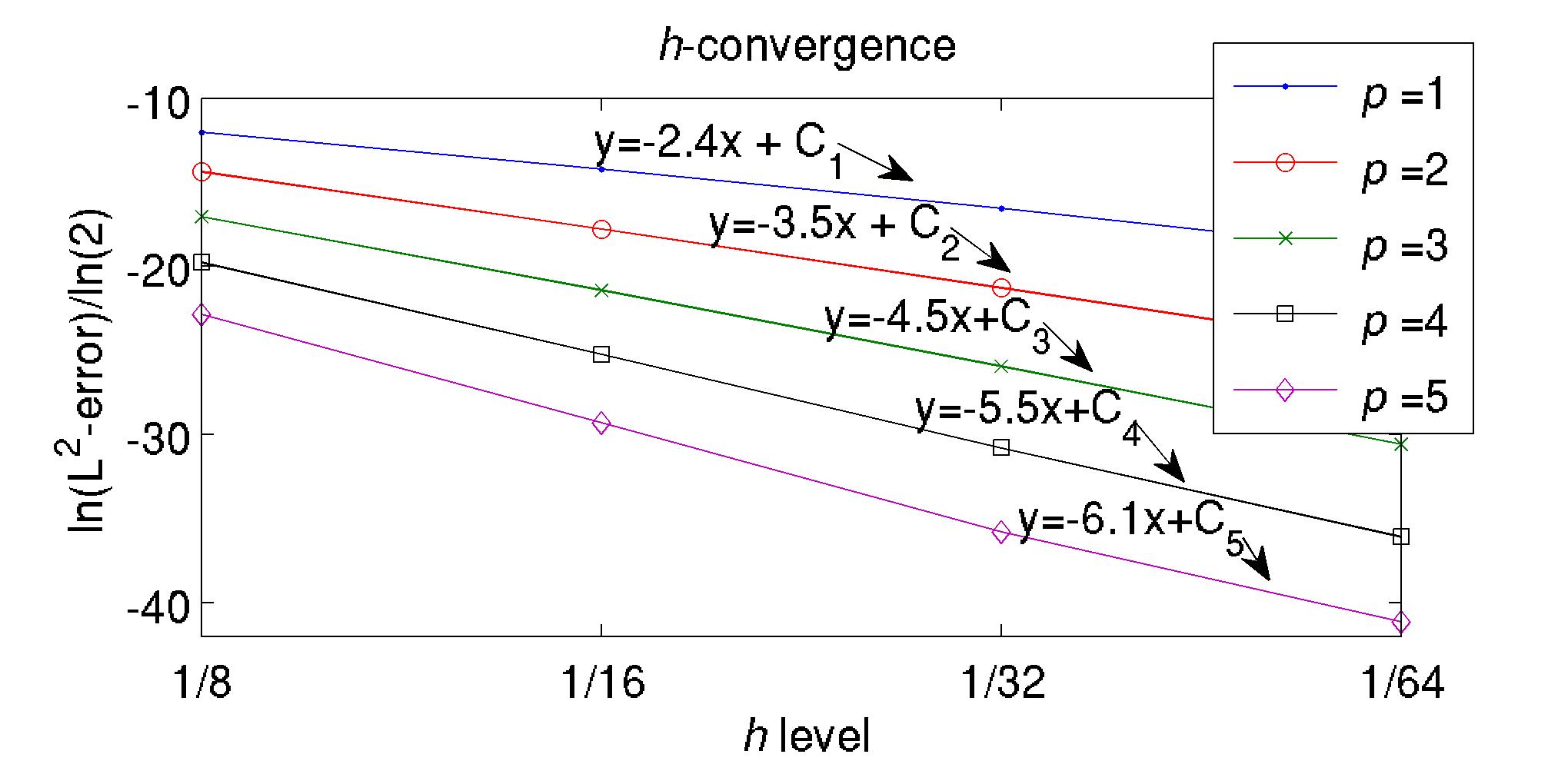
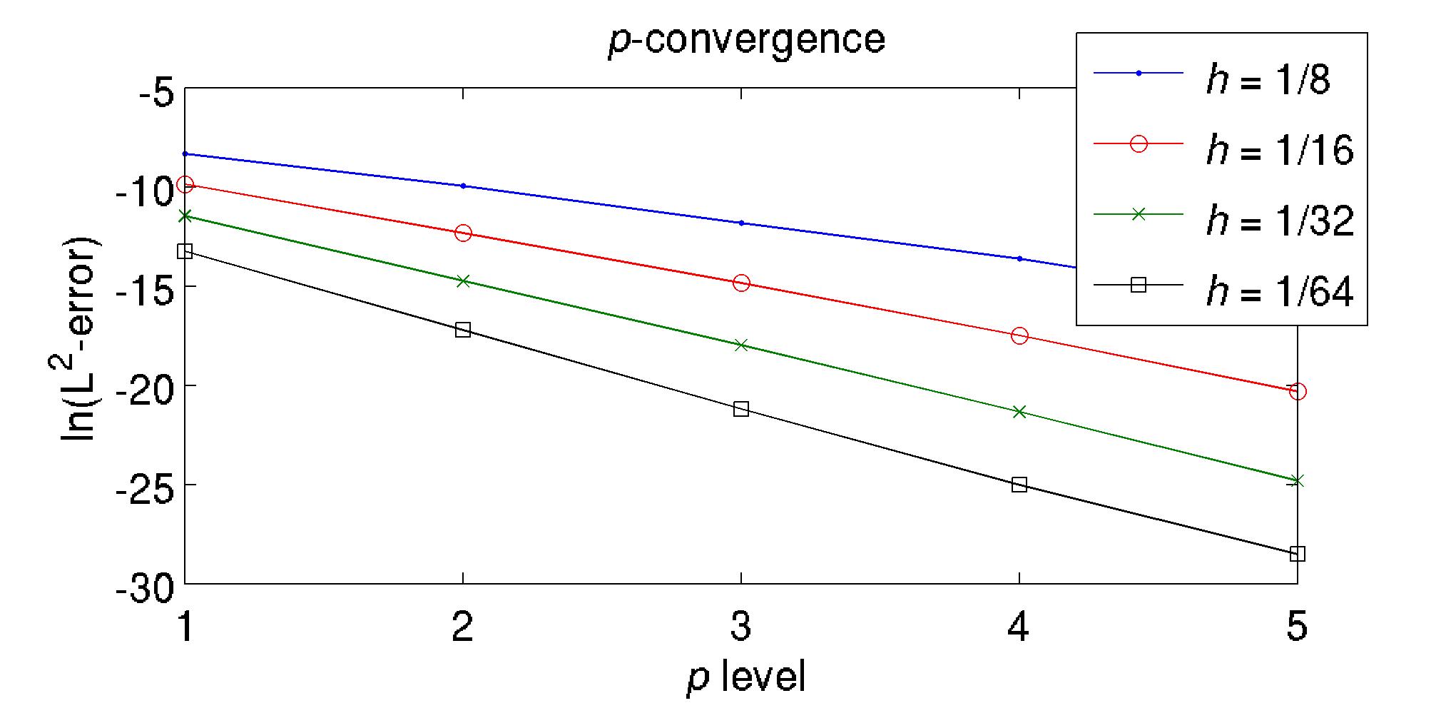
Refer to caption
Figure 8: The regression rates of convergence for the p∈{1,
,5}𝑝1
5p\in\{1,\ldots,5\} cases are given by the slope of a linear regression line taken from the data in Table 1.
Refer to caption
Figure 9: The convergence in p∈{1,
,5}𝑝1
5p\in\{1,\ldots,5\} for the different mesh sizes, as taken from the data in Table 1.
p𝑝p L2/L∞superscript𝐿2superscript𝐿L^{2}/L^{\infty}–error Ll​o​c2subscriptsuperscript𝐿2𝑙𝑜𝑐L^{2}_{loc} projection error x=1/hđ‘„1ℎx=1/h
1 1.76×10⁻⁶/5.31×10−81.76superscript1065.31superscript1081.76\times 10^{-6}/5.31\times 10^{-8} 4.57×10−74.57superscript1074.57\times 10^{-7} 64
2 3.34×10⁻⁸/4.75×10−103.34superscript1084.75superscript10103.34\times 10^{-8}/4.75\times 10^{-10} 1.63×10−111.63superscript10111.63\times 10^{-11} 64
3 6.24×10⁻¹⁰/3.19×10−116.24superscript10103.19superscript10116.24\times 10^{-10}/3.19\times 10^{-11} 8.61×10−158.61superscript10158.61\times 10^{-15} 64
4 1.36×10⁻¹¹/1.63×10−121.36superscript10111.63superscript10121.36\times 10^{-11}/1.63\times 10^{-12} 8.22×10−198.22superscript10198.22\times 10^{-19} 64
5 4.14×10⁻¹³/6.54×10−144.14superscript10136.54superscript10144.14\times 10^{-13}/6.54\times 10^{-14} 5.31×10−225.31superscript10225.31\times 10^{-22} 64
1 1.05×10⁻⁵/6.84×10−71.05superscript1056.84superscript1071.05\times 10^{-5}/6.84\times 10^{-7} 7.12×10−67.12superscript1067.12\times 10^{-6} 32
2 3.94×10⁻⁷/1.10×10−83.94superscript1071.10superscript1083.94\times 10^{-7}/1.10\times 10^{-8} 1.07×10−91.07superscript1091.07\times 10^{-9} 32
3 1.55×10⁻⁸/3.79×10−101.55superscript1083.79superscript10101.55\times 10^{-8}/3.79\times 10^{-10} 2.16×10−122.16superscript10122.16\times 10^{-12} 32
4 5.35×10⁻¹⁰/2.49×10−115.35superscript10102.49superscript10115.35\times 10^{-10}/2.49\times 10^{-11} 8.52×10−168.52superscript10168.52\times 10^{-16} 32
5 1.67×10⁻¹¹/1.42×10−121.67superscript10111.42superscript10121.67\times 10^{-11}/1.42\times 10^{-12} 2.12×10−182.12superscript10182.12\times 10^{-18} 32
1 5.24×10⁻⁵/6.17×10−65.24superscript1056.17superscript1065.24\times 10^{-5}/6.17\times 10^{-6} 1.07×10−41.07superscript1041.07\times 10^{-4} 16
2 4.44×10⁻⁶/2.78×10−74.44superscript1062.78superscript1074.44\times 10^{-6}/2.78\times 10^{-7} 6.85×10−86.85superscript1086.85\times 10^{-8} 16
3 3.56×10⁻⁷/2.31×10−83.56superscript1072.31superscript1083.56\times 10^{-7}/2.31\times 10^{-8} 5.12×10−105.12superscript10105.12\times 10^{-10} 16
4 2.55×10⁻⁸/5.73×10−102.55superscript1085.73superscript10102.55\times 10^{-8}/5.73\times 10^{-10} 8.78×10−138.78superscript10138.78\times 10^{-13} 16
5 1.50×10⁻⁹/4.36×10−111.50superscript1094.36superscript10111.50\times 10^{-9}/4.36\times 10^{-11} 7.89×10−157.89superscript10157.89\times 10^{-15} 16
1 2.39×10⁻⁴/5.17×10−52.39superscript1045.17superscript1052.39\times 10^{-4}/5.17\times 10^{-5} 1.30×10−31.30superscript1031.30\times 10^{-3} 8
2 4.73×10⁻⁵/6.89×10−64.73superscript1056.89superscript1064.73\times 10^{-5}/6.89\times 10^{-6} 3.54×10−63.54superscript1063.54\times 10^{-6} 8
3 7.36×10⁻⁶/7.58×10−77.36superscript1067.58superscript1077.36\times 10^{-6}/7.58\times 10^{-7} 9.55×10−89.55superscript1089.55\times 10^{-8} 8
4 1.21×10⁻⁶/6.41×10−81.21superscript1066.41superscript1081.21\times 10^{-6}/6.41\times 10^{-8} 5.98×10−105.98superscript10105.98\times 10^{-10} 8
5 1.32×10⁻⁷/6.07×10−91.32superscript1076.07superscript1091.32\times 10^{-7}/6.07\times 10^{-9} 2.19×10−112.19superscript10112.19\times 10^{-11} 8
Table 1: We show the convergence results for the hℎh and p𝑝p levels whose errors are bounded by machine precision after 64 timesteps. The Ll​o​c2subscriptsuperscript𝐿2𝑙𝑜𝑐L^{2}_{loc} projection error into the basis is also included, though, as is clear, these errors are often below machine double precision (∌1.11×10⁻¹⁶similar-toabsent1.11superscript1016\sim 1.11\times 10^{-16}), and hence not particularly meaningful.

4.2 §​4.2§4.2\S 4.2 The rotating half annular crest, cone, and hill solution

Here we solve a standard rotating landscape solution to a scalar transport equation. That is, consider the hyperbolic advection problem:

∂tÎč+𝒖⋅∇xÎč=0,subscript𝑡𝜄⋅𝒖subscriptâˆ‡đ‘„đœ„0\partial_{t}\iota+\boldsymbol{u}\cdot\nabla_{x}\iota=0, (4.1)

with initial-boundary data given by

Îč|t=0=Îč0,andÎčb=0,\iota_{|t=0}=\iota_{0},\quad\mathrm{and}\quad\iota_{b}=0,

corresponding to vanishing boundary data, given a time-independent velocity vector field 𝒖=𝒖​(𝒙)𝒖𝒖𝒙\boldsymbol{u}=\boldsymbol{u}(\boldsymbol{x}) with the transported scalar quantity Îč=Îč​(t,𝒙)𝜄𝜄𝑡𝒙\iota=\iota(t,\boldsymbol{x}) in dimension two, such that 𝒙=(x,y)đ’™đ‘„đ‘Š\boldsymbol{x}=(x,y) and 𝒖=(u,v)𝒖𝑱𝑣\boldsymbol{u}=(u,v).

p𝑝p Limiter type L2​errorL∞​errorsuperscript𝐿2errorsuperscript𝐿error\frac{L^{2}\mathrm{error}}{L^{\infty}\mathrm{error}} Limiter type L2​errorL∞​errorsuperscript𝐿2errorsuperscript𝐿error\frac{L^{2}\mathrm{error}}{L^{\infty}\mathrm{error}}
1 BJ limiter[6],§3.2 (1.5×10−30.73)1.5superscript1030.73\left(\frac{1.5\times 10^{-3}}{0.73}\right) Adapted BJ§3.2.1 (1.5×10−30.73)1.5superscript1030.73\left(\frac{1.5\times 10^{-3}}{0.73}\right)
1 DEO limiter[12] (1.1×10−30.71)1.1superscript1030.71\left(\frac{1.1\times 10^{-3}}{0.71}\right) BDS limiter[7],§3.4 (5.9×10−40.67)5.9superscript1040.67\left(\frac{5.9\times 10^{-4}}{0.67}\right)
1 Vertex[25, 28],§3.2 (1.1×10−30.73)1.1superscript1030.73\left(\frac{1.1\times 10^{-3}}{0.73}\right) Adapted vertex§3.2.1 (1.0×10−30.72)1.0superscript1030.72\left(\frac{1.0\times 10^{-3}}{0.72}\right)
1 Recombination§3.5 (5.9×10−40.67)5.9superscript1040.67\left(\frac{5.9\times 10^{-4}}{0.67}\right) ReconstructionMUSCL [1, 27],§3.3 (5.9×10−40.67)5.9superscript1040.67\left(\frac{5.9\times 10^{-4}}{0.67}\right)
2 BJ limiter[6],§3.2 (2.3×10−30.74)2.3superscript1030.74\left(\frac{2.3\times 10^{-3}}{0.74}\right) Restriction [7],§3.4 (5.0×10−40.64)5.0superscript1040.64\left(\frac{5.0\times 10^{-4}}{0.64}\right)
2 Vertex [25, 28],§3.2 (2.3×10−30.73)2.3superscript1030.73\left(\frac{2.3\times 10^{-3}}{0.73}\right) Adapted vertex§3.2.1 (2.3×10−30.74)2.3superscript1030.74\left(\frac{2.3\times 10^{-3}}{0.74}\right)
2 Recombination§3.5 (2.2×10−30.74)2.2superscript1030.74\left(\frac{2.2\times 10^{-3}}{0.74}\right) ReconstructionENO [1, 27],§3.3 (2.3×10−30.73)2.3superscript1030.73\left(\frac{2.3\times 10^{-3}}{0.73}\right)
3 BJ limiter[6],§3.2 (2.6×10−30.72)2.6superscript1030.72\left(\frac{2.6\times 10^{-3}}{0.72}\right) Restriction [7],§3.4 (4.7×10−40.73)4.7superscript1040.73\left(\frac{4.7\times 10^{-4}}{0.73}\right)
3 Vertex [25, 28],§3.2 (2.6×10−30.72)2.6superscript1030.72\left(\frac{2.6\times 10^{-3}}{0.72}\right) Adapted vertex§3.2.1 (2.5×10−30.73)2.5superscript1030.73\left(\frac{2.5\times 10^{-3}}{0.73}\right)
3 Recombination§3.5 (2.6×10−30.72)2.6superscript1030.72\left(\frac{2.6\times 10^{-3}}{0.72}\right) ReconstructionENO [1, 27],§3.3 (2.2×10−30.75)2.2superscript1030.75\left(\frac{2.2\times 10^{-3}}{0.75}\right)
4 BJ limiter[6],§3.2 (2.8×10−30.72)2.8superscript1030.72\left(\frac{2.8\times 10^{-3}}{0.72}\right) Restriction [7],§3.4 (4.8×10−40.69)4.8superscript1040.69\left(\frac{4.8\times 10^{-4}}{0.69}\right)
4 Vertex [25, 28],§3.2 (2.9×10−30.72)2.9superscript1030.72\left(\frac{2.9\times 10^{-3}}{0.72}\right) Adapted vertex§3.2.1 (2.8×10−30.72)2.8superscript1030.72\left(\frac{2.8\times 10^{-3}}{0.72}\right)
4 Recombination§3.5 (2.9×10−40.72)2.9superscript1040.72\left(\frac{2.9\times 10^{-4}}{0.72}\right) ReconstructionENO [1, 27],§3.3 (2.6×10−30.73)2.6superscript1030.73\left(\frac{2.6\times 10^{-3}}{0.73}\right)
Table 2: We give the L2superscript𝐿2L^{2} and L∞superscript𝐿L^{\infty}-errors of the approximate solutions after one full rotation with respect to (4.1), setting h=1/256ℎ1256h=1/256, Δ​t=1×10⁻³Δ𝑡1superscript103\Delta t=1\times 10^{-3} and using Runge–Kutta SSP(5,3)53(5,3). The error ratio for the solution with no limiter at p=1𝑝1p=1 is L2/L∞=2.55×10−4/0.61superscript𝐿2superscript𝐿2.55superscript1040.61L^{2}/L^{\infty}=2.55\times 10^{-4}/0.61, at p=2𝑝2p=2 is L2/L∞=2.28×10−4/0.44superscript𝐿2superscript𝐿2.28superscript1040.44L^{2}/L^{\infty}=2.28\times 10^{-4}/0.44, at p=3𝑝3p=3 is L2/L∞=1.71×10−4/0.35superscript𝐿2superscript𝐿1.71superscript1040.35L^{2}/L^{\infty}=1.71\times 10^{-4}/0.35, and for p>3𝑝3p>3 is unstable. Though, as expected, the error in the stable unlimited solutions concentrate along the discontinuities demonstrating sharp (≄10%absentpercent10\geq 10\% cell-wise in Îč𝜄\iota) overshoots and undershoots.
Refer to caption
Refer to caption
Refer to caption
Refer to caption
Refer to caption
Refer to caption
Figure 10: Here we show the p=1𝑝1p=1 results from Table 2 after one full revolution. The upper left is the exact L2superscript𝐿2L^{2} projection at p=1𝑝1p=1, the top right is the DEO limiter[12], the middle left is the vertex limiter[25, 28],§3.2, the middle right the BDS limiter[7],§3.4, the bottom left the adapted vertex limiter§3.2.1, and the bottom right the BJ limiter[6],§3.2.

We choose a simple square domain Ω=[−12,12]2Ωsuperscript12122\Omega=\big{[}-\frac{1}{2},\frac{1}{2}\big{]}^{2}, with velocity field 𝒖=(y,−x)đ’–đ‘Šđ‘„\boldsymbol{u}=(y,-x). Then letting τđ’Ș=π/4subscript𝜏đ’Ș𝜋4\tau_{\mathcal{O}}=\pi/4 and defining the auxiliary variables

đ’Șx=x​cosâĄÏ„đ’Ș−y​sinâĄÏ„đ’Șandđ’Șy=y​cosâĄÏ„đ’Ș+x​sinâĄÏ„đ’Ș,formulae-sequencesubscriptđ’Șđ‘„đ‘„subscript𝜏đ’Ș𝑩subscript𝜏đ’Șandsubscriptđ’Ș𝑩𝑩subscript𝜏đ’Șđ‘„subscript𝜏đ’Ș\mathcal{O}_{x}=x\cos\tau_{\mathcal{O}}-y\sin\tau_{\mathcal{O}}\quad\mathrm{and}\quad\mathcal{O}_{y}=y\cos\tau_{\mathcal{O}}+x\sin\tau_{\mathcal{O}},

we take initial data satisfying:

Îč0={1,if​A,1−B​a−1,if​B≀a,14​(1+cosâĄÏ€â€‹r),otherwise,\iota_{0}=\left\{\begin{matrix}1,&\mathrm{if}\ A,\\ 1-Ba^{-1},&\mathrm{if}\ B\leq a,\\ \frac{1}{4}\left(1+\cos{\pi r}\right),&\mathrm{otherwise},\end{matrix}\right. (4.2)

where

A=𝐮absent\displaystyle A= (a0≀B≀a)∧(đ’Șx≀a1),B=(đ’Șx−14)2+đ’Șy2,subscript𝑎0đ”đ‘Žsubscriptđ’Șđ‘„subscript𝑎1đ”superscriptsubscriptđ’Șđ‘„142superscriptsubscriptđ’Ș𝑩2\displaystyle\left(a_{0}\leq B\leq a\right)\land\left(\mathcal{O}_{x}\leq a_{1}\right),\qquad B=\sqrt{\left(\mathcal{O}_{x}-\frac{1}{4}\right)^{2}+\mathcal{O}_{y}^{2}},

and

r=a−1​min⁥(a,đ’Șx2+(đ’Șy+1/4)2),𝑟superscript𝑎1𝑎superscriptsubscriptđ’Șđ‘„2superscriptsubscriptđ’Ș𝑩142r=a^{-1}\min\left(a,\sqrt{\mathcal{O}_{x}^{2}+(\mathcal{O}_{y}+1/4)^{2}}\right),

taking a=0.18𝑎0.18a=0.18, a0=0.025subscript𝑎00.025a_{0}=0.025 and a1=−0.23subscript𝑎10.23a_{1}=-0.23.

The exact solution may be determined by noticing that since for any F​(x,y)đčđ‘„đ‘ŠF(x,y), where x=x​(t)đ‘„đ‘„đ‘Ąx=x(t) and y=y​(t)𝑩𝑩𝑡y=y(t), that

d​Fd​t=∂tF+(xâ€Čyâ€Č)​∇F=0,𝑑đč𝑑𝑡subscript𝑡đčmatrixsuperscriptđ‘„â€Čsuperscript𝑩â€Č∇đč0\frac{dF}{dt}=\partial_{t}F+\begin{pmatrix}x^{\prime}\\ y^{\prime}\end{pmatrix}\nabla F=0,

which implies that for

𝒖=(uv)=(y−x),we​have​the​systemxâ€Č=yandyâ€Č=−x,formulae-sequence𝒖matrix𝑱𝑣matrixđ‘Šđ‘„wehavethesystemsuperscriptđ‘„â€Č𝑩andsuperscript𝑩â€Čđ‘„\boldsymbol{u}=\begin{pmatrix}u\\ v\end{pmatrix}=\begin{pmatrix}y\\ -x\end{pmatrix},\quad\mathrm{we\ have\ the\ system}\quad x^{\prime}=y\quad\mathrm{and}\quad y^{\prime}=-x,

that may be solved by recombining such that the solution to the second order ODE, yâ€Čâ€Č+y=0superscript𝑩â€Čâ€Č𝑩0y^{\prime\prime}+y=0 can be viewed as a generator of the rotation matrix R𝑅R about the origin. That is, we obtain the clockwise transformation

R=(cos⁡t−sin⁡tsin⁡tcos⁡t),𝑅matrix𝑡𝑡𝑡𝑡R=\begin{pmatrix}\cos t&-\sin t\\ \sin t&\cos t\end{pmatrix}, (4.3)

such that R​𝒙𝑅𝒙R\boldsymbol{x} yields the exact solution.

Refer to caption
Refer to caption
Refer to caption
Refer to caption
Refer to caption
Refer to caption
Figure 11: Here we show the p=2𝑝2p=2 to p=4𝑝4p=4 results from Table 2 after one full revolution. The left column shows the linear restriction of the BDS limiter[7],§3.4 in descending order, while the right column shows the next best limiter, in descending order, i.e. at p=2𝑝2p=2, p=3𝑝3p=3 and p=4𝑝4p=4 the hierarchical reconstructionENO [1, 27],§3.3.

For our numerical experiments, we follow a similar case to that presented in [25] setting our mesh width to h=1/128ℎ1128h=1/128 and Δ​t=1×10⁻³Δ𝑡1superscript103\Delta t=1\times 10^{-3} in keeping with the CFL condition on hyperbolic transport (e.g. see [38]) ). Let us briefly discuss the results shown in Figure 10 and Figure 11 and Table 2. We note that we have run all of our experiments on a regular structured triangular grid.

In Figure 10 we see the results for linears. The Durlofsky–Engquist–Osher[12] limiter, the vertex limiter [25] and the adapted vertex limiter seem to show qualitatively similar behaviors. The Barth–Jespersen limiter [6] is slightly more diffuse here at linears (where the adapted Barth–Jespersen shows only slight improvement over the native Barth–Jespersen limiter as well), while the BDS limiter [7] described in §3.4 shows by far the best L2superscript𝐿2L^{2}–error behavior and clearly maintains the best signature behavior of the solution everywhere but at the points of discontinuity, where these values are tightly redistributed. As previously suggested [25] the vertex limiter and the Barth–Jespersen limiter are both quite sensitive to mesh geometries, where the former is better suited in some sense to geometries with “sharp angles,” and the latter (the Barth–Jespersen limiter) is well-suited for regular structured meshes (e.g. Delaunay triangulations). However, because of the so–called “blind diffusion” of both these regimes caused by local extrema — as discussed in §3.2.1 — this behavior is not entirely predictable or monotone with respect to mesh regularity, as we see below. The hierarchic linear recombination from §3.5, and the hierarchical reconstruction from §3.3 are both equivalent by construction to the BDS limiter at p=1𝑝1p=1.

When p>1𝑝1p>1 we see an immediate and substantial degradation in the limiting behavior of all the regimes, with the single exception of the linear restriction of the BDS limiter from §3.4. This is immediately prevalent at p=2𝑝2p=2, where the hierarchic linear recombination method from §3.3 is the next best limiting regime and yet has an L2superscript𝐿2L^{2}-error more than four times that of the linear restriction. In fact, the hierarchical reconstruction method from §3.3 may be the most natural extension of the BDS limiter to order p𝑝p, where the choice of linearization is the most direct application of the BDS scheme in the Taylor basis. But even here, where at p=2𝑝2p=2 we have added only three more degrees of freedom to the polynomial hierarchical basis, we see that performing the limiter on the linear reconstructions — which amounts to performing the limiting procedure on only two more components (i.e. the linear components which are limited with respect to their respective slopes) — shows a substantial loss locally in the sharpness of the resolution along the discontinuities.

The reason for this loss of resolution is not entirely mysterious or unexpected, though previous work [25] has demonstrated geometries where this degradation is not immediately observable at p=2𝑝2p=2, and this behavior seems related to the mass lumping strategy previously discussed in §3.2.1 (which deserves closer analysis). Nevertheless, here we see that as p𝑝p increases the number of applications of the limiter to the solution increases as a function of the degrees of freedom at the (p−1)𝑝1(p-1)-st degree (i.e. (p−1)​(p−2)/2𝑝1𝑝22(p-1)(p-2)/2). In fact this is true for each of the limiting regimes, with the exception of the hierarchical reconstruction methods from §3.3, which actually perform yet another iteration of the limiter by employing one of the minmod functions at top order. However, the hierarchical reconstruction methods also seem to benefit from the fact that they utilize information coming from nonlinearities present in the solution at every level by linearizing with respect to these nonlinearities (e.g. equation (3.30)) — in contrast to the vertex-based schemes which linearize about a single monomial component (3.21) of the expansion, and then utilize a regularizing constraint such as (3.24). It turns out that the addition of this nonlinear signature behavior at higher order seems to allow the hierarchical reconstruction methods to capture the profile more completely, even with the additional application of the limiting regime at each timestep.

However, by far the most effective limiting regime for p>1𝑝1p>1 is the linear restriction of the BDS limiter from §3.4, where in ℜℜ\mathfrak{R} the Î”đœ€\varepsilon has been set to 10−4superscript10410^{-4}. Again, this result is not entirely unexpected, since slope limiting, as its name suggests, finds its roots in limiting the slopes of lines with respect to some linear basis [40]. That having been said, it then seems unlikely that one should be able to expect an improvement in the accuracy of a solution near a sharp front simply by applying the slope limiter more frequently to the linearization of its respective monomial components. Since, for example, if one assumes (fairly realistically) that the top order component has an approximately fixed order error which is introduced upon application of the limiter to the FEM solution, then each subsequent application of the limiter to the lower level đ”©đ”©\mathfrak{l} components should only be able to increase the subsequent error introduced over all. In the hierarchical reconstruction methods of [1, 27], on the other hand, the componentwise minmod function attenuates this effect somewhat, as does the fact that all of the limited higher order components serve to help limit the lower order components at every level đ”©đ”©\mathfrak{l}.

Before discussing this further, let us first confirm that this result is not simply a special case of (4.1) which demonstrates a pathological behavior with respect to (4.2). Below we take a solution with admits a number of additional types of singular submanifolds that help to further explicate each limiter’s behavior.

4.3 §​4.3§4.3\S 4.3 Steady state convective torque

Now we show a steady state solution to equation (4.1), which effectively isolates the error present in the form of torque away from the steady (discontinuous) state in a rotating constant frame solution. Our goal here is to present a more difficult set of singular submanifolds ℬi⊂ℬsubscriptℬ𝑖ℬ\mathcal{B}_{i}\subset\mathcal{B} present with respect to a steady state solution (where the solution here is thought of as the base manifold ℬℬ\mathcal{B}) in order to more completely isolate the error explicitly introduced by the limiting regimes over varying order p𝑝p.

Here we work over the Cartesian domain Ω=[0,2]×[−1,1]Ω0211\Omega=[0,2]\times[-1,1], given the same boundary conditions from §4.1, and where the exact steady solution is characterized by a velocity field satisfying 𝒖=(y,1−x)𝒖𝑩1đ‘„\boldsymbol{u}=(y,1-x) and a steady state scalar field Îč𝜄\iota given by:

Îč={2−23​r,if​r≀a12​a1​(1+cos⁥[(r−a2)​π]),if​a1<r≀3.5​a33​a1,if​ 4​a3≀r≀2​a13​a3​(1+cos⁥[(r−a2)​π]),6​a3≀r≀7​a3a1,if​ 8​a3≀r≀9​a30,otherwise\iota=\left\{\begin{matrix}2-\frac{2}{3}r,&\mathrm{if}\ r\leq a_{1}\\ 2a_{1}\left(1+\cos{[(r-a_{2})\pi]}\right),&\mathrm{if}\ a_{1}<r\leq 3.5a_{3}\\ 3a_{1},&\mathrm{if}\ 4a_{3}\leq r\leq 2a_{1}\\ 3a_{3}\left(1+\cos{[(r-a_{2})\pi]}\right),&6a_{3}\leq r\leq 7a_{3}\\ a_{1},&\mathrm{if}\ 8a_{3}\leq r\leq 9a_{3}\\ 0,&\mathrm{otherwise}\end{matrix}\right. (4.4)

where

r=(x−1)2+(y)2,a1=14,a2=133anda3=110.formulae-sequence𝑟superscriptđ‘„12superscript𝑩2formulae-sequencesubscript𝑎114formulae-sequencesubscript𝑎2133andsubscript𝑎3110r=\sqrt{(x-1)^{2}+(y)^{2}},\quad a_{1}=\frac{1}{4},\quad a_{2}=\frac{13}{3}\quad\mathrm{and}\quad a_{3}=\frac{1}{10}.
p𝑝p Limiter type L2​errorL∞​errorsuperscript𝐿2errorsuperscript𝐿error\frac{L^{2}\mathrm{error}}{L^{\infty}\mathrm{error}} Limiter type L2​errorL∞​errorsuperscript𝐿2errorsuperscript𝐿error\frac{L^{2}\mathrm{error}}{L^{\infty}\mathrm{error}}
1 BJ limiter[6],§3.2 (1.2×10−20.49)1.2superscript1020.49\left(\frac{1.2\times 10^{-2}}{0.49}\right) Vertex[25, 28],§3.2 (1.2×10−20.51)1.2superscript1020.51\left(\frac{1.2\times 10^{-2}}{0.51}\right)
1 DEO limiter[12] (1.0×10−20.47)1.0superscript1020.47\left(\frac{1.0\times 10^{-2}}{0.47}\right) BDS limiter[7],§3.4 (6.8×10−30.40)6.8superscript1030.40\left(\frac{6.8\times 10^{-3}}{0.40}\right)
1 Recombination§3.5 (6.8×10−30.40)6.8superscript1030.40\left(\frac{6.8\times 10^{-3}}{0.40}\right) ReconstructionENO [1, 27],§3.3 (6.8×10−30.40)6.8superscript1030.40\left(\frac{6.8\times 10^{-3}}{0.40}\right)
2 BJ limiter[6],§3.2 (1.9×10−20.50)1.9superscript1020.50\left(\frac{1.9\times 10^{-2}}{0.50}\right) Restriction [7],§3.4 (6.6×10−30.38)6.6superscript1030.38\left(\frac{6.6\times 10^{-3}}{0.38}\right)
2 Vertex [25, 28],§3.2 (1.9×10−20.50)1.9superscript1020.50\left(\frac{1.9\times 10^{-2}}{0.50}\right) Adapted vertex§3.2.1 (1.9×10−20.50)1.9superscript1020.50\left(\frac{1.9\times 10^{-2}}{0.50}\right)
2 Recombination§3.5 (1.9×10−20.50)1.9superscript1020.50\left(\frac{1.9\times 10^{-2}}{0.50}\right) ReconstructionENO [1, 27],§3.3 (1.8×10−20.52)1.8superscript1020.52\left(\frac{1.8\times 10^{-2}}{0.52}\right)
3 BJ limiter[6],§3.2 (2.2×10−20.50)2.2superscript1020.50\left(\frac{2.2\times 10^{-2}}{0.50}\right) Restriction [7],§3.4 (7.7×10−30.39)7.7superscript1030.39\left(\frac{7.7\times 10^{-3}}{0.39}\right)
3 Vertex [25, 28],§3.2 (2.3×10−20.50)2.3superscript1020.50\left(\frac{2.3\times 10^{-2}}{0.50}\right) Adapted vertex§3.2.1 (2.2×10−20.50)2.2superscript1020.50\left(\frac{2.2\times 10^{-2}}{0.50}\right)
3 Recombination§3.5 (2.3×10−20.50)2.3superscript1020.50\left(\frac{2.3\times 10^{-2}}{0.50}\right) ReconstructionENO [1, 27],§3.3 (2.2×10−20.51)2.2superscript1020.51\left(\frac{2.2\times 10^{-2}}{0.51}\right)
4 BJ limiter[6],§3.2 (2.3×10−20.50)2.3superscript1020.50\left(\frac{2.3\times 10^{-2}}{0.50}\right) Restriction [7],§3.4 (7.7×10−30.38)7.7superscript1030.38\left(\frac{7.7\times 10^{-3}}{0.38}\right)
4 Vertex [25, 28],§3.2 (2.3×10−20.50)2.3superscript1020.50\left(\frac{2.3\times 10^{-2}}{0.50}\right) Adapted vertex§3.2.1 (2.3×10−20.50)2.3superscript1020.50\left(\frac{2.3\times 10^{-2}}{0.50}\right)
4 Recombination§3.5 (2.3×10−20.50)2.3superscript1020.50\left(\frac{2.3\times 10^{-2}}{0.50}\right) ReconstructionENO [1, 27],§3.3 (2.2×10−20.51)2.2superscript1020.51\left(\frac{2.2\times 10^{-2}}{0.51}\right)
Table 3: We give the L2superscript𝐿2L^{2} and L∞superscript𝐿L^{\infty}-errors of the approximate solutions after T𝑇T corresponding to a 1/4141/4 rotation with respect to (4.4), setting h=1/128ℎ1128h=1/128, Δ​t=5×10⁻⁴Δ𝑡5superscript104\Delta t=5\times 10^{-4} and using Runge–Kutta SSP(5,3)53(5,3). The error ratio for the solution with no limiter at p=1𝑝1p=1 is L2/L∞=3.9×10−3/0.40superscript𝐿2superscript𝐿3.9superscript1030.40L^{2}/L^{\infty}=3.9\times 10^{-3}/0.40, at p=2𝑝2p=2 is L2/L∞=2.9×10−3/0.34superscript𝐿2superscript𝐿2.9superscript1030.34L^{2}/L^{\infty}=2.9\times 10^{-3}/0.34, at p=3𝑝3p=3 is L2/L∞=2.4×10−3/0.23superscript𝐿2superscript𝐿2.4superscript1030.23L^{2}/L^{\infty}=2.4\times 10^{-3}/0.23, and for p>3𝑝3p>3 is unstable. Again, as in Table 2, the unlimited solutions are dominated by local overshoots and undershoots along the discontinuities.

The solution ℬℬ\mathcal{B} as shown in Figure 12 is augmented from the relatively well-behaved circular convection case analyzed in [25]. Here we have similar outer rings (though substantially “thinned”), but have supplemented a pair of inner ring submanifolds that have a thickness of no more than a single point that similarly intersects an inner cone along a line of singular points, and with a very thin island outer ring. These initial conditions are not particularly well-behaved, as can be seen in Figure 12, where even in the L2superscript𝐿2L^{2}–projected exact solution at p=7𝑝7p=7 there are variations (jagged lines) at the mesh resolution along the lines of singular points. To compound this, we use a larger domain than that of [25], which effectively doubles the velocity of the pseudo-timestepping in the y𝑩y-direction, providing for even more instability in the solution space.

Note that in Figure 12 and Figure 13, the asymmetry in the solution is merely due to that fact that we have only gone a quarter turn, thus the diffusive signature of each limiter has only been advected a quarter turn, and accumulates or dissipates according to the local behavior of the advective flux.

Now, notice that the adapted limiters from §3.2.1 are not well–suited to handle (4.4) at all. In fact (3.26) is, in particular, adapted to represent a case which almost always leads to problems, since it does not deal differentially with the special case of Ui,bmax=Ui,bminsubscriptsuperscript𝑈𝑖𝑏subscriptsuperscript𝑈𝑖𝑏U^{\max}_{i,b}=U^{\min}_{i,b}, which in (3.26) up to the resolution hℎh is the case for nearly every element in the domain, leading to an almost globally uniform “blind diffusion.” In fact the adapted cases are almost identical to the native cases at low p𝑝p — when not explicitly dealing with Ui,bmax=Ui,bminsubscriptsuperscript𝑈𝑖𝑏subscriptsuperscript𝑈𝑖𝑏U^{\max}_{i,b}=U^{\min}_{i,b} — even though the native vertex and Barth–Jespersen limiters do not recognize local extrema at all, while the adapted cases do recognize local extrema up to, but not including, the degenerate case of Ui,bmax=Ui,bminsubscriptsuperscript𝑈𝑖𝑏subscriptsuperscript𝑈𝑖𝑏U^{\max}_{i,b}=U^{\min}_{i,b}. As p𝑝p increases the repeated iterations of the limiter swamps this behavior in both the native and adapted limiters, and thus the solutions converge to the same value. It is possible that a mass lumping strategy might mitigate some of these affects (see [25] for more information on this technique).
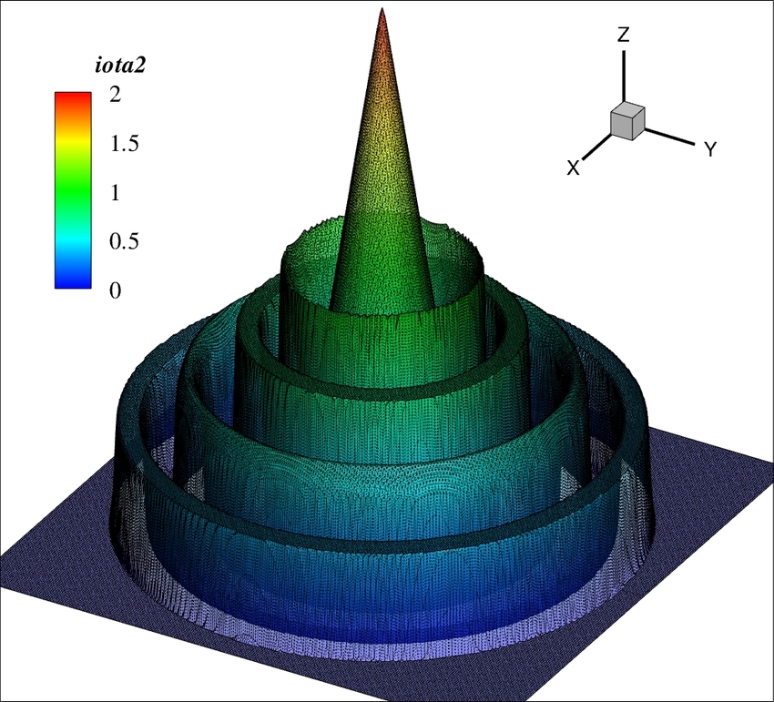
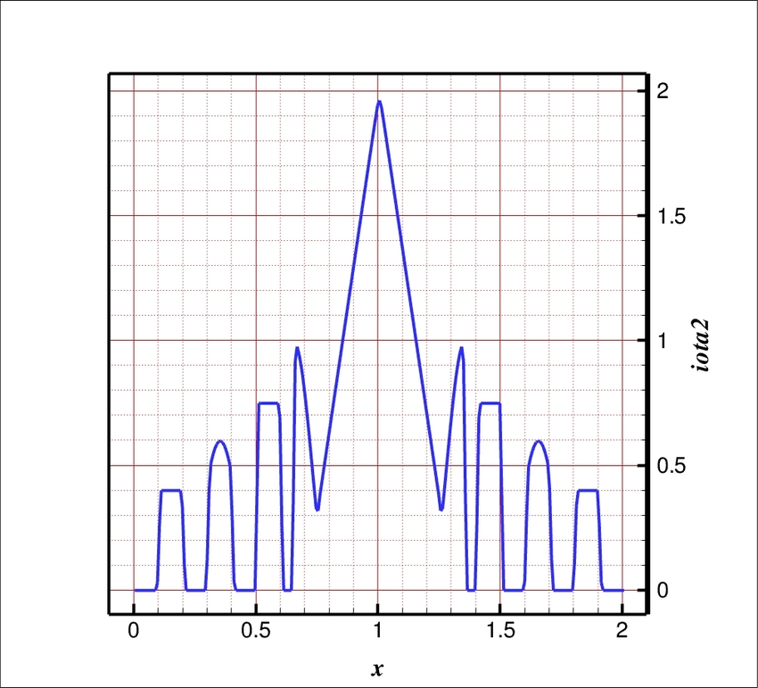
Refer to caption
Refer to caption
Refer to caption
Refer to caption
Refer to caption
Refer to caption
Figure 12: Here at top we show the L2superscript𝐿2L^{2}–projection of the exact solution at p=7𝑝7p=7, with the x​zđ‘„đ‘§xz–plane slice on the right after 1/4141/4 turn. The middle shows the p=1𝑝1p=1 case of the linear restriction [7],§3.4, and the bottom shows the p=1𝑝1p=1 DEO limiter[12].
Refer to caption
Refer to caption
Refer to caption
Refer to caption
Refer to caption
Refer to caption
Figure 13: At top we show the p=4𝑝4p=4 linear restriction after 1/4141/4 turn. The middle shows the p=3𝑝3p=3 linear reconstruction [1, 27],§3.3, and the bottom the p=2𝑝2p=2 linear recombination§3.5.

Moreover, in this example (4.4) the Barth–Jespersen limiter is clearly initially more diffuse than the native vertex limiter, which is primarily due here to the fact that the singular submanifolds are chosen such that they — again up to the mesh resolution hℎh — spatially oscillate on a local neighborhood which is larger than the characteristic length of the edge neighborhood, and so the focal neighborhood is a more appropriate area to “sense” in order to capture this semi-localized signature behavior. Moreover, the problem of local extrema as discussed in §3.2.1 is of lesser importance in this case, since up to the set of codimension one submanifolds of ΩhsubscriptΩℎ\Omega_{h} in (4.4), the entire domain is characterized and dominated by extremely sharp profiles, making the diffusion — which is potentially “blind” near smooth regions — more appropriate here. However, again as p𝑝p increases this behavior gets swamped by the repeated iterations.

The linear restriction of the BDS limiter[7],§3.4 once again demonstrates the best limiting behavior as a function of increasing p𝑝p, which again seems to emphasize the fact that limiting a solution for p>1𝑝1p>1 must somehow account for the implicit nonlinearity present internal to the cell in a relatively explicit way; or, at least, a way which is fully functionally coupled to the entire solution as it exists everywhere on the local cell.

Nevertheless, the linear restriction still substantially outperforms all of the competing limiting regimes. There seems to be some indication here that, at least presently, one may expect that near areas dominated by shocks the best accuracy that one can hope for is linear accuracy, while still hoping to preserve physically important characteristics of the solution (e.g. positivity perserving, local conservation of mass, etc.). Of interest, is that this observation falls very neatly in line with the state of the art in h​pℎ𝑝hp–adaptive numerical schemes, where a general heuristic follows that for potentially discontinuous solutions, in areas of high cell–wise variability, the local order of p𝑝p is only increased if inter–element jumps are small or bounded and controlled, and the internal cell-wise variation is strictly bounded above by the cell(s) (usually a subset of cells) containing the global maximum [10, 30].

We explore this issue some in the subsequent section as it applies to p𝑝p–enrichment, though we also note that at present we are not aware of any formal results which come anywhere near to formulating a theorem that subsumes this observational fact (which may in general prove to be only one part of the story). Nevertheless, such a result would be of substantial importance to the field, as would a counter example, which here could simply be the development of a fully p𝑝p convergent slope limiting regime that limits at all levels đ”©đ”©\mathfrak{l} while still preserving the important physical features of the solution (and of course does so without relying on prior knowledge, such as the existence of an exact solution).

5 §​5§5\S 5 Adjoining the dynamic p𝑝p-enrichment

Here we present a number of generalizable p𝑝p-enrichment/de–enrichment schemes based on local data and apply them to the problems from §4. These p𝑝p-enrichment schemes may be viewed as alternatives to, for example, the specific energy methods presented in [30] which rely upon the variational global entropy of the system of equations, and those discussed in [11] and [5, 19], which, as in [30], try to maximally enrich the domain based on global solution behavior taken with respect to the available computational resources and either a priori or a posteriori estimates.

5.1 A general approach based on local data

We implement a dynamic p𝑝p-enrichment scheme that utilizes a number of different methodologies in order to capture higher order structure in areas of “permissible variability.” This scheme is built with respect to our collection of p𝑝p-adaptive slope limiters from §3, such that we inherently arrive with a dynamically limited p𝑝p-enriched solution.

The nuance of implementing such a scheme in the generalized formulation is that the solution must demonstrate a minimal smoothness condition in areas of p𝑝p-enrichment, while in areas approaching discontinuity, p𝑝p-enrichment must be suppressed in order to maintain stability (especially in the absence of a limiter). This issue is not a concern of course when one is able to make smoothness assumptions a priori about the entire solution space over Ω×(0,T)Ω0𝑇\Omega\times(0,T) (viz. the formalism of [9] and [23]), and has been shown to demonstrate very nice behavior especially in solution spaces which are not only smooth, but where in particular one would like to resolve stable areas of maximal variation (e.g. as are applicable in some storm surge model applications [23]).

Nevertheless, in the context of a slightly more generalized system of equations with, for example, a coupled hyperbolic equation (or possessing a hyperbolic character in a system of equations) such as (4.1), such assumptions cannot generally be made over the entire discrete solution space over Ωh×(0,T)subscriptΩℎ0𝑇\Omega_{h}\times(0,T), since areas demonstrating strong local gradients ∇xđ‘Œhsubscriptâˆ‡đ‘„subscriptđ‘Œâ„Ž\nabla_{x}\boldsymbol{U}_{h} may indicate the presence or formation of numeric shock fronts (even given smooth initial data), in which case local p𝑝p-enrichment has a destabilizing effect on the solution (that is, the weak approximation to a discontinuity becomes more ill-behaved with respect to increasing p𝑝p).

Here we are concerned with dynamically p𝑝p-adapted solutions to the generalized formulation of (LABEL:aprox) and (LABEL:SSPRK) in conjunction with the slope limiters presented in §3. We implement a very simple set of p𝑝p–enrichment strategies, which as we will see, generally tend to undersample the variational space (e.g. in contrast to, for example, the poor man’s or poor man’s greedy algorithm of [11] which always adapts based on some percentage of a global relative bound). The reason for this simplification here is to reduce the number of varying parameters in the scheme, in order to isolate the stability of the solution with respect to the limiting schemes of §3. Hence, we simply set hard tolerances which do not depend on, for example, the available computational resources or global bounds on the solution.

Now, in order to additionally deal with both smooth and discontinuous initial–boundary data (as well as smooth and discontinuous solutions in (0,T)0𝑇(0,T)) we implement the following two distinct dynamic p𝑝p-enrichment schemes — namely we designate them: Type I and Type II p𝑝p-enrichment schemes. We also note that in this section all functions are defined with respect to the master element ℳℳ\mathcal{M} representation.

The first type of enrichment scheme (i.e. Type I ) applies to solutions in which smoothness may be assumed a priori over the entire domain Ω×(0,T)Ω0𝑇\Omega\times(0,T). That is, taking the approximate solution vector đ‘Œhsubscriptđ‘Œâ„Ž\boldsymbol{U}_{h} we compute the auxiliary sensor over each i𝑖i-th component of of the state variable đ‘Œđ‘Œ\boldsymbol{U} (having m𝑚m components, as in §2):

Πji=|đ‘Œhi|ωjâˆ’đ‘Œhi|cχj|,subscriptsuperscriptΠ𝑖𝑗evaluated-atsuperscriptsubscriptđ‘Œâ„Žđ‘–subscript𝜔𝑗evaluated-atsuperscriptsubscriptđ‘Œâ„Žđ‘–đ‘subscript𝜒𝑗\Pi^{i}_{j}=\bigg{|}\frac{\boldsymbol{U}_{h}^{i}|_{\omega_{j}}-\boldsymbol{U}_{h}^{i}|_{c}}{\chi_{j}}\bigg{|}, (5.1)

where c𝑐c is the centroid of element ΩesubscriptÎ©đ‘’\Omega_{e} and ωjsubscript𝜔𝑗\omega_{j} is the midpoint of the j𝑗j–th edge of ΩesubscriptÎ©đ‘’\Omega_{e}, and the solution đ‘Œhsubscriptđ‘Œâ„Ž\boldsymbol{U}_{h} is evaluated at these two points, respectively. For smooth solutions, the function χjsubscript𝜒𝑗\chi_{j} may be set to either the distance χj=|ωj−c|subscript𝜒𝑗subscript𝜔𝑗𝑐\chi_{j}=|\omega_{j}-c| as in [23], or the product χj=ωj​csubscript𝜒𝑗subscript𝜔𝑗𝑐\chi_{j}=\omega_{j}c as in [9]. In either case, over each timestep n𝑛n the following p𝑝p-enrichment functional 𝔈el=𝔈el​(đ’«k​(Ωeln))subscript𝔈subscript𝑒𝑙subscript𝔈subscript𝑒𝑙superscriptđ’«đ‘˜superscriptsubscriptΩsubscript𝑒𝑙𝑛\mathfrak{E}_{e_{l}}=\mathfrak{E}_{e_{l}}(\mathscr{P}^{k}(\Omega_{e_{l}}^{n})) is evaluated over each cell ΩelsubscriptΩsubscript𝑒𝑙\Omega_{e_{l}}:

Type I p𝑝p-enrichment 𝔈el={đ’«k+1​(Ωeln)if​((supisupjΠji≄ϔ)∧(k+1≀pmax))√(τ0≄tw),đ’«k−1​(Ωeln)if​(infisupjΠji<Ï”)∧(k−1≄pmin)∧(τ0≄tw),đ’«k​(Ωeln)otherwise,\mathfrak{E}_{e_{l}}=\left\{\begin{matrix}\mathscr{P}^{k+1}(\Omega_{e_{l}}^{n})&\mathrm{if}\ \left((\sup_{i}\sup_{j}\Pi^{i}_{j}\geq\epsilon)\land(k+1\leq p_{\max})\right)\lor\left(\tau_{0}\geq t^{w}\right),\\ \mathscr{P}^{k-1}(\Omega_{e_{l}}^{n})&\mathrm{if}\ (\inf_{i}\sup_{j}\Pi^{i}_{j}<\epsilon)\land(k-1\geq p_{\min})\land(\tau_{0}\geq t^{w}),\\ \mathscr{P}^{k}(\Omega_{e_{l}}^{n})&\ \mathrm{otherwise,}\end{matrix}\right. (5.2)

where τ0subscript𝜏0\tau_{0} is a counter that restricts the p𝑝p enrichment/de-enrichment such that it may only occur every twsuperscriptđ‘Ąđ‘€t^{w} timesteps, and where k∈{1,
,p}𝑘1
𝑝k\in\{1,\ldots,p\}.

For solutions demonstrating approximately nonzero local approximate gradients ∇xđ‘Œh≠0subscriptâˆ‡đ‘„subscriptđ‘Œâ„Ž0\nabla_{x}\boldsymbol{U}_{h}\neq 0, wherein we might expect local discontinuities we must find an estimate of the local relative “smoothness” of đ‘Œhsubscriptđ‘Œâ„Ž\boldsymbol{U}_{h}. One way of doing this is by setting the auxiliary sensor equal to the following Van Leer minmod function across elements (as used in [9]):

Πji=minmod​(đ‘Œhi|vj+âˆ’đ‘Œhi|c,đ‘Œhi|vjâˆ’âˆ’đ‘Œhi|c),subscriptsuperscriptΠ𝑖𝑗minmodevaluated-atsubscriptsuperscriptđ‘Œđ‘–â„Žsuperscriptsubscript𝑣𝑗evaluated-atsubscriptsuperscriptđ‘Œđ‘–â„Žđ‘evaluated-atsubscriptsuperscriptđ‘Œđ‘–â„Žsuperscriptsubscript𝑣𝑗evaluated-atsubscriptsuperscriptđ‘Œđ‘–â„Žđ‘\Pi^{i}_{j}=\mathrm{minmod}(\boldsymbol{U}^{i}_{h}|_{v_{j}^{+}}-\boldsymbol{U}^{i}_{h}|_{c},\boldsymbol{U}^{i}_{h}|_{v_{j}^{-}}-\boldsymbol{U}^{i}_{h}|_{c}), (5.3)

where vjsubscript𝑣𝑗v_{j} is the j𝑗j–th vertex of ΩelsubscriptΩsubscript𝑒𝑙\Omega_{e_{l}}. As Πij→0→superscriptsubscriptΠ𝑖𝑗0\Pi_{i}^{j}\to 0 the solution becomes smoother, and one may subsequently employ (5.2).

A slightly simpler method of dealing with discontinuous solutions simply using local information is to define a local smoothness estimator (as discussed in [41] and [33]) such that we again may calculate an elementwise version of (5.1) depending only on the the interior of ΩelsubscriptΩsubscript𝑒𝑙\Omega_{e_{l}}, such that:

Πiel=(â€–đ‘Œhiâˆ’đ‘ŒË˜hi‖Lq​(Ωel)â€–đ‘Œhi‖Lq​(Ωel)),superscriptsubscriptΠ𝑖subscript𝑒𝑙subscriptnormsubscriptsuperscriptđ‘Œđ‘–â„ŽsubscriptsuperscriptË˜đ‘Œđ‘–â„Žsuperscript𝐿𝑞subscriptΩsubscript𝑒𝑙subscriptnormsubscriptsuperscriptđ‘Œđ‘–â„Žsuperscript𝐿𝑞subscriptΩsubscript𝑒𝑙\Pi_{i}^{e_{l}}=\left(\frac{\|\boldsymbol{U}^{i}_{h}-\breve{\boldsymbol{U}}^{i}_{h}\|_{L^{q}(\Omega_{e_{l}})}}{\|\boldsymbol{U}^{i}_{h}\|_{L^{q}(\Omega_{e_{l}})}}\right), (5.4)

for the Lqsuperscript𝐿𝑞L^{q} norms (except when q=2𝑞2q=2 in which case we take the standard inner product, as used in our examples below), where đ‘ŒË˜hsubscriptË˜đ‘Œâ„Ž\breve{\boldsymbol{U}}_{h} is the elementwise projected solution đ’«k−1​(Ωeln)superscriptđ’«đ‘˜1superscriptsubscriptΩsubscript𝑒𝑙𝑛\mathscr{P}^{k-1}(\Omega_{e_{l}}^{n}), such that in our mixed version (5.2) becomes:

Type II p𝑝p-enrichment 𝔈el={đ’«k+1​(Ωeln)if​(supilog10⁥Πiel≀A)∧(k+1≀pmax),đ’«k−1​(Ωeln)if​(infilog10⁥Πiel≄A)∧(k−1≄pmin)∧(τ0≄tw),đ’«k​(Ωeln)otherwise,\mathfrak{E}_{e_{l}}=\left\{\begin{matrix}\mathscr{P}^{k+1}(\Omega_{e_{l}}^{n})&\mathrm{if}\ (\sup_{i}\log_{10}\Pi^{e_{l}}_{i}\leq A)\land(k+1\leq p_{\max}),\\ \mathscr{P}^{k-1}(\Omega_{e_{l}}^{n})&\mathrm{if}\ (\inf_{i}\log_{10}\Pi^{e_{l}}_{i}\geq A)\land(k-1\geq p_{\min})\land(\tau_{0}\geq t^{w}),\\ \mathscr{P}^{k}(\Omega_{e_{l}}^{n})&\ \mathrm{otherwise,}\end{matrix}\right. (5.5)

where the bound satisfies

A={log10⁡c~​k−q2+c,for​p>pminsupilog10⁡Πiel,otherwiseA=\left\{\begin{matrix}\log_{10}\tilde{c}k^{-q^{2}}+c,&\mathrm{for}\ p>p_{\min}\\ \sup_{i}\log_{10}\Pi^{e_{l}}_{i},&\mathrm{otherwise}\end{matrix}\right. (5.6)

such that c~,c∈ℝ+~𝑐𝑐superscriptℝ\tilde{c},c\in\mathbb{R}^{+} are user defined constants, where c~∈(0,10)~𝑐010\tilde{c}\in(0,10) is recommended (see for example [41]) for resolving discontinuities in the context of h​pℎ𝑝hp-adaptivity, and where we have found c∈(−2,2)𝑐22c\in(-2,2) optimal. The basic intuition that underpins the use of (5.4) is the observation that discontinuous basis functions are assumed to decay, for smooth solutions, at a rate comparable to that of the Fourier coefficients in a standard expansion of the solution — which clearly decay at a rate of 1/k41superscript𝑘41/k^{4} for q=2𝑞2q=2 (see [41, 33, 34]), to which we obtain an indicator of the relative local regularity of the solution, i.e. the faster the coefficients decay, the smoother the local solution. Thus we obtain equation (5.4), which approaches zero as the solution becomes smoother, where setting c>0𝑐0c>0 is a sharper restriction than the more permissive (i.e. less stable) condition c<0𝑐0c<0.

Refer to caption
Refer to caption
Refer to caption
Refer to caption
Figure 14: Here we show the p𝑝p values mapped over the p=1𝑝1p=1, L2superscript𝐿2L^{2}-projected profiles at T=0.003𝑇0.003T=0.003 on the top solutions, and at T=0.06𝑇0.06T=0.06 on the bottom solutions using the settings given in Table 4. The solutions on the left use the Type II p𝑝p-enrichment, and those on the right use the Type I p𝑝p-enrichment.
p𝑝p Limiter type Type I, L2superscript𝐿2L^{2} Type II, L2superscript𝐿2L^{2} Ï”italic-Ï”\epsilon c𝑐c, c~~𝑐\tilde{c} twsuperscriptđ‘Ąđ‘€t^{w} q𝑞q
1–5 BJ limiter[6],§3.2 3.66×10−33.66superscript1033.66\times 10^{-3} 2.18×10−32.18superscript1032.18\times 10^{-3} 0.1 -1 0.1 0 2
1–5 Vertex[25, 28],§3.2 3.10×10−33.10superscript1033.10\times 10^{-3} 2.10×10−32.10superscript1032.10\times 10^{-3} 0.1 -1 0.1 0 2
1–5 Restriction [7],§3.4 X 8.03×10−48.03superscript1048.03\times 10^{-4} 0.1 -1 0.1 0 2
1–5 Recombination§3.5 2.17×10−32.17superscript1032.17\times 10^{-3} 2.09×10−32.09superscript1032.09\times 10^{-3} 0.1 -1 0.1 0 2
1–5 ReconstructionENO [1, 27],§3.3 1.98×10−31.98superscript1031.98\times 10^{-3} 1.91×10−31.91superscript1031.91\times 10^{-3} 0.1 -1 0.1 0 2
Table 4: We give the L2superscript𝐿2L^{2}-errors of the approximate solutions after T𝑇T corresponding to a 1/4141/4 rotation with p𝑝p-enrichment on (4.4), setting h=1/128ℎ1128h=1/128, Δ​t=5×10⁻⁴Δ𝑡5superscript104\Delta t=5\times 10^{-4} and using Runge–Kutta SSP(5,3)53(5,3).

The results are shown in Table 4 and Figure 14. As expected from before, the linear restriction from §3.4 is again by far the most accurate of the choice of limiters when it is stable, where it is important to note that in the p𝑝p-enrichment case the restriction function ℜℜ\mathfrak{R} from §3.4 is calculated using Δ=10−4𝜀superscript104\varepsilon=10^{-4}, which has the effect of passing cells containing steep gradients to the dynamic p𝑝p-enrichment functions 𝔈𝔈\mathfrak{E}. This is enough, it turns out, to make the Type I p𝑝p-enrichment regime unstable with respect to the dynamically adaptive linear restriction limiting regime from §3.3 due in part to the function of ℜℜ\mathfrak{R}, which creates an unstable p𝑝p-flickering along sharp profile edges. However, even turning off the p𝑝p-de-enriching functionality of ℜℜ\mathfrak{R} does not help in this case, since the linear restriction still zeros out the higher order components, which in the Type I case effectively still allows p𝑝p to flicker locally, leading to the formation of instabilities along sharp edges. We also note that in Table 4 we have suppressed the L∞superscript𝐿L^{\infty}-error, as numerical experimentation suggests that very small changes in the p𝑝p-enrichment settings Ï”,c,c~,italic-Ï”đ‘~𝑐\epsilon,c,\tilde{c}, and twsuperscriptđ‘Ąđ‘€t^{w} can cause big shifts in Ll​o​c∞superscriptsubscript𝐿𝑙𝑜𝑐L_{loc}^{\infty}, which make the L∞superscript𝐿L^{\infty}-error a deceptive measure in the discontinuous p𝑝p-enrichment case.

Finally, we emphasize that the p𝑝p-enriched slope limited solutions show substantially better accuracy than the constant-in-p𝑝p solutions from §4.2. This can be attributed in large part to the observation that the majority of error in the solutions is accumulated along the discontinuities, which is precisely where the p𝑝p-enrichement schemes p𝑝p-transition between levels (see Figure 14). Hence, in both Type I and Type II cases (i.e. spatially, from either side of the discontinuity) the p𝑝p-enrichement strongly attenuates (by explicit truncation) the oscillatory instabilities present in these regions, as long as the solution does not flicker unstably between them.

6 §​6§6\S 6 Conclusion

We have presented a discontinuous Galerkin finite element method for solving dynamically p𝑝p-enriched solutions with consistent slope limiting to arbitrary order in two spatial dimensions over generalized coupled systems of PDEs. We have provided a formalism for transforming between the polynomial basis of different regimes in order to move between representation spaces. We then introduced, up to but not including a substantial choice of minmod functions, seven dynamic-in-p𝑝p slope limiting regimes, and performed numerical experiments on these regimes in order to develop a sense of their strengths and weaknesses. We found that our numerical results suggest that, given discontinuous initial data, slope limiting over fixed order solutions when p>1𝑝1p>1 is most effectively accomplished by restricting back to the linear case and using a sharp limiter in that regime, rather than keeping the higher order data and trying to limit it in a consistent way — which we found introduces more numerical diffusion (i.e. error) on average over time.

We then presented two types of p𝑝p-enrichment schemes, fully coupled to the above slope limiting regimes. These schemes are designed to exploit certain properties of the solution, and simple algorithms were implemented. We then tested these coupled systems on the same model problem in order to develop a sense of how dynamic-in-p𝑝p systems perform relative to fixed-in-p𝑝p systems. Here again, we found that restricting to the linear case seems to be the most effective (and also, incidentally, efficient) way of limiting a dynamically p𝑝p-adapting solution. Moreover, we found that in general using the Type I and Type II methods of p𝑝p-enrichment the accuracy of the solution was substantially improved (i.e. by an order of magnitude) with respect to the native solution using only the dynamic-in-p𝑝p slope limiters of §3.

Future directions include taking the slope limited solution from §3 coupled to the p𝑝p-enrichment scheme from §5 and adding dynamic hℎh-adaptivity to it, in order to fully exploit the power of h​pℎ𝑝hp-adaptive convergence.

7 §​7§7\S 7 Acknowledgements

The first author would like to thank P.G. Schmitz, Wenhao Wang, Troy Butler, Corey Trahan, Nishant Panda and Jennifer Proft for helpful conversations. The authors would also like to aknowledge the support of the National Science Foundation grants OCI-0749075 and OCI-0746232.

References

  • Abgrall [1994] R. Abgrall. On essentially non-oscillatory schemes on unstructured meshes: analysis and implementation. J. Comput. Phys., 114(1):45–58, 1994. ISSN 0021-9991. doi: 10.1006/jcph.1994.1148. URL http://dx.doi.org/10.1006/jcph.1994.1148.
  • Aizinger and Dawson [2002] V. Aizinger and C. Dawson. A discontinuous Galerkin method for two-dimensional flow and transport in shallow water. Advances in Water Resources, 25(1):67 – 84, 2002. ISSN 0309-1708. doi: 10.1016/S0309-1708(01)00019-7. URL http://www.sciencedirect.com/science/article/B6VCF-44PK3KB-5/2/51beaaea%1191c299bcd3a0d40beca43d.
  • Arnold et al. [2000] D.N. Arnold, F. Brezzi, B. Cockburn, and D. Marini. Discontinuous Galerkin methods for elliptic problems. In Discontinuous Galerkin methods (Newport, RI, 1999), volume 11 of Lect. Notes Comput. Sci. Eng., pages 89–101. Springer, Berlin, 2000.
  • Ballestra and Sacco [2004] L.V. Ballestra and R. Sacco. Numerical problems in semiconductor simulation using the hydrodynamic model: a second-order finite difference scheme. J. Comput. Phys., 195(1):320–340, 2004. ISSN 0021-9991. doi: 10.1016/j.jcp.2003.10.002. URL http://dx.doi.org/10.1016/j.jcp.2003.10.002.
  • Bangerth and Kayser-Herold [2009] W. Bangerth and O. Kayser-Herold. Data structures and requirements for hp finite element software. ACM Trans. Math. Softw., 36:4:1–4:31, March 2009. ISSN 0098-3500. doi: http://doi.acm.org/10.1145/1486525.1486529. URL http://doi.acm.org/10.1145/1486525.1486529.
  • Barth and Jesperson [1989] T. Barth and D.C. Jesperson. The design and application of upwind schemes and unstructured meshes. AIAA paper, volume 89–0366, pages 1–12, 1989.
  • Bell et al. [1988] J.B. Bell, C.N. Dawson, and G.R. Shubin. An unsplit, higher order Godunov method for scalar conservation laws in multiple dimensions. Journal of Computational Physics, 74(1):1 – 24, 1988. ISSN 0021-9991. doi: 10.1016/0021-9991(88)90065-4. URL http://www.sciencedirect.com/science/article/B6WHY-4DD1T8P-N0/2/aba1bf5%19b0924a0a20968665aa37091.
  • Bunya et al. [2009] S. Bunya, E.J. Kubatko, J. J. Westerink, and C. Dawson. A wetting and drying treatment for the Runge-Kutta discontinuous Galerkin solution to the shallow water equations. Comput. Methods Appl. Mech. Engrg., 198(17-20):1548–1562, 2009. ISSN 0045-7825. doi: 10.1016/j.cma.2009.01.008. URL http://dx.doi.org/10.1016/j.cma.2009.01.008.
  • Burbeau and Sagaut [2005] A. Burbeau and P. Sagaut. A dynamic p𝑝p-adaptive discontinuous Galerkin method for viscous flow with shocks. Comput. & Fluids, 34(4-5):401–417, 2005. ISSN 0045-7930. doi: 10.1016/j.compfluid.2003.04.002. URL http://dx.doi.org/10.1016/j.compfluid.2003.04.002.
  • Demkowicz [2007] L. Demkowicz. Computing with h​pℎ𝑝hp-adaptive finite elements. Vol. 1. Chapman & Hall/CRC Applied Mathematics and Nonlinear Science Series. Chapman & Hall/CRC, Boca Raton, FL, 2007. ISBN 978-1-58488-671-6; 1-58488-671-4. One and two dimensional elliptic and Maxwell problems, With 1 CD-ROM (UNIX).
  • Demkowicz [2010] L. Demkowicz. A new discontinuous Petrov-Galerkin method with optimal test functions. part v: solution of 1D Burgers’ and Navier-Stokes equations. page 34, 2010. URL http://www.ices.utexas.edu/media/reports/2010/1025.pdf.
  • Durlofsky et al. [1992] L.J. Durlofsky, B. Engquist, and S. Osher. Triangle based adaptive stencils for the solution of hyperbolic conservation laws. Journal of Computational Physics, 98(1):64 – 73, 1992. ISSN 0021-9991. doi: 10.1016/0021-9991(92)90173-V. URL http://www.sciencedirect.com/science/article/B6WHY-4DD1P88-NW/2/14f5775%efbf9049e31e12411e2e34238.
  • Feistauer et al. [2003] M. Feistauer, J. Felcman, and I. StraĆĄkraba. Mathematical and computational methods for compressible flow. Numerical mathematics and scientific computation. Oxford University Press, 2003. ISBN 0-19-850588-4.
  • Ghostine et al. [2009] R. Ghostine, G. Kesserwani, R. MosĂ©, J. Vazquez, and A. Ghenaim. An improvement of classical slope limiters for high-order discontinuous Galerkin method. Internat. J. Numer. Methods Fluids, 59(4):423–442, 2009. ISSN 0271-2091. doi: 10.1002/fld.1823. URL http://dx.doi.org/10.1002/fld.1823.
  • Godoy and DesJardin [2010] W.F. Godoy and P.E. DesJardin. On the use of flux limiters in the discrete ordinates method for 3D radiation calculations in absorbing and scattering media. J. Comput. Phys., 229(9):3189–3213, 2010. ISSN 0021-9991. doi: 10.1016/j.jcp.2009.12.037. URL http://dx.doi.org/10.1016/j.jcp.2009.12.037.
  • Hoteit et al. [2004] H. Hoteit, Ph. Ackerer, R. MosĂ©, J. Erhel, and B. Philippe. New two-dimensional slope limiters for discontinuous Galerkin methods on arbitrary meshes. Internat. J. Numer. Methods Engrg., 61(14):2566–2593, 2004. ISSN 0029-5981. doi: 10.1002/nme.1172. URL http://dx.doi.org/10.1002/nme.1172.
  • Isoardi et al. [2010] L. Isoardi, G. Chiavassa, G. Ciraolo, P. Haldenwang, E. Serre, Ph. Ghendrih, Y. Sarazin, F. Schwander, and P. Tamain. Penalization modeling of a limiter in the Tokamak edge plasma. J. Comput. Phys., 229(6):2220–2235, 2010. ISSN 0021-9991. doi: 10.1016/j.jcp.2009.11.031. URL http://dx.doi.org/10.1016/j.jcp.2009.11.031.
  • Jin and Xu [2007] C. Jin and K. Xu. A unified moving grid gas-kinetic method in Eulerian space for viscous flow computation. J. Comput. Phys., 222(1):155–175, 2007. ISSN 0021-9991. doi: 10.1016/j.jcp.2006.07.015. URL http://dx.doi.org/10.1016/j.jcp.2006.07.015.
  • Kanschat [2004] G. Kanschat. Multilevel methods for discontinuous galerkin fem on locally refined meshes. Computers & Structures, 82(28):2437 – 2445, 2004. ISSN 0045-7949. doi: 10.1016/j.compstruc.2004.04.015. URL http://www.sciencedirect.com/science/article/B6V28-4DBJGG5-4/2/5cb85d27%cc196137146048cd3d9d4c33. Preconditioning methods: algorithms, applications and software environments.
  • Kubatko et al. [2006] E.J. Kubatko, J.J. Westerink, and C. Dawson. h​pℎ𝑝hp discontinuous Galerkin methods for advection dominated problems in shallow water flow. Computer Methods in Applied Mechanics and Engineering, 196(1-3):437 – 451, 2006. ISSN 0045-7825. doi: 10.1016/j.cma.2006.05.002. URL http://www.sciencedirect.com/science/article/B6V29-4M1CYTM-1/2/6c45c85d%20d17690046881a795b0b04d.
  • Kubatko et al. [2007a] E.J. Kubatko, J.J. Westerink, and C. Dawson. Semi discrete discontinuous Galerkin methods and stage-exceeding-order, strong-stability-preserving Runge-Kutta time discretizations. J. Comput. Phys., 222(2):832–848, 2007a. ISSN 0021-9991. doi: 10.1016/j.jcp.2006.08.005. URL http://dx.doi.org/10.1016/j.jcp.2006.08.005.
  • Kubatko et al. [2008] E.J. Kubatko, C. Dawson, and J.J. Westerink. Time step restrictions for Runge-Kutta discontinuous Galerkin methods on triangular grids. J. Comput. Phys., 227(23):9697–9710, 2008. ISSN 0021-9991. doi: 10.1016/j.jcp.2008.07.026. URL http://dx.doi.org/10.1016/j.jcp.2008.07.026.
  • Kubatko et al. [2009a] E.J. Kubatko, S. Bunya, C. Dawson, and J.J. Westerink. Dynamic p-adaptive Runge-Kutta discontinuous Galerkin methods for the shallow water equations. Computer Methods in Applied Mechanics and Engineering, 198(21-26):1766 – 1774, 2009a. ISSN 0045-7825. doi: 10.1016/j.cma.2009.01.007. URL http://www.sciencedirect.com/science/article/B6V29-4VDY7X4-1/2/36e49328%fea4e4f751d689510b7e3b3f. Advances in Simulation-Based Engineering Sciences - Honoring J. Tinsley Oden.
  • Kubatko et al. [2009b] E.J. Kubatko, S. Bunya, C. Dawson, J.J. Westerink, and C. Mirabito. A performance comparison of continuous and discontinuous finite element shallow water models. J. Sci. Comput., 40(1-3):315–339, 2009b. ISSN 0885-7474. doi: 10.1007/s10915-009-9268-2. URL http://dx.doi.org/10.1007/s10915-009-9268-2.
  • Kuzmin [2010] D. Kuzmin. A vertex-based hierarchical slope limiter for p𝑝p-adaptive discontinuous Galerkin methods. J. Comput. Appl. Math., 233(12):3077–3085, 2010. ISSN 0377-0427. doi: http://dx.doi.org/10.1016/j.cam.2009.05.028.
  • Levy et al. [2004] D. Levy, C.-W. Shu, and J. Yan. Local discontinuous Galerkin methods for nonlinear dispersive equations. J. Comput. Phys., 196(2):751–772, 2004. ISSN 0021-9991.
  • Liu et al. [2007] Y. Liu, C.-W. Shu, E. Tadmor, and M. Zhang. Central discontinuous Galerkin methods on overlapping cells with a nonoscillatory hierarchical reconstruction. SIAM J. Numer. Anal., 45(6):2442–2467 (electronic), 2007. ISSN 0036-1429. doi: 10.1137/060666974. URL http://dx.doi.org/10.1137/060666974.
  • Luo et al. [2008] H. Luo, J. Baum, and R. Löhner. A discontinuous Galerkin method based on a Taylor basis for the compressible flows on arbitrary grids. Journal of Computational Physics, 227(20):8875 – 8893, 2008. ISSN 0021-9991. doi: 10.1016/j.jcp.2008.06.035. URL http://www.sciencedirect.com/science/article/B6WHY-4T13CS3-2/2/cacbb700%cf043776d94ac1bd3a985bed.
  • Michoski et al. [2009] C. Michoski, J.A. Evans, P.G. Schmitz, and A. Vasseur. Quantum hydrodynamics with trajectories: the nonlinear conservation form mixed/discontinuous Galerkin method with applications in chemistry. J. Comput. Phys., 228(23):8589–8608, 2009. ISSN 0021-9991. doi: 10.1016/j.jcp.2009.08.011. URL http://dx.doi.org/10.1016/j.jcp.2009.08.011.
  • Michoski et al. [2010a] C. Michoski, J.A. Evans, and P.G. Schmitz. Multiscale discontinuous Galerkin h​pℎ𝑝hp–adaptive chemical reacters I: quiescent reactors. preprint, 2011a.
  • Michoski et al. [2010b] C. Michoski, J.A. Evans, P.G. Schmitz, and A. Vasseur. A discontinuous Galerkin method for viscous compressible multifluids. J. Comput. Phys., 229(6):2249–2266, 2010b. ISSN 0021-9991. doi: 10.1016/j.jcp.2009.11.033. URL http://dx.doi.org/10.1016/j.jcp.2009.11.033.
  • Murillo et al. [2009] J. Murillo, P. GarcĂ­a-Navarro, and J. Burguete. Conservative numerical simulation of multi-component transport in two-dimensional unsteady shallow water flow. J. Comput. Phys., 228(15):5539–5573, 2009. ISSN 0021-9991. doi: 10.1016/j.jcp.2009.04.039. URL http://dx.doi.org/10.1016/j.jcp.2009.04.039.
  • Palaniappan et al. [2008] J. Palaniappan, S.T. Miller, and R.B. Haber. Sub-cell shock capturing and spacetime discontinuity tracking for nonlinear conservation laws. Internat. J. Numer. Methods Fluids, 57(9):1115–1135, 2008. ISSN 0271-2091. doi: 10.1002/fld.1850. URL http://dx.doi.org/10.1002/fld.1850.
  • Persson and Peraire [2006] P.P. Persson and J. Peraire. Sub-cell shock capturing for discontinuous Galerkin methods. Forty-fourth AIAA Aerospace Sciences Meeting and Exhibit, Reno, NV, U.S.A., Online:5––18, 2006.
  • Qiu and Shu [2005] J. X. Qiu and C. W. Shu. Runge-kutta discontinuous Galerkin method using WENO limiters. Siam J. On Scientific Computing, 26(3):907–929, 2005.
  • Ruuth [2006] S.J. Ruuth. Global optimization of explicit strong-stability-preserving Runge-Kutta methods. Math. Comp., 75(253):183–207 (electronic), 2006. ISSN 0025-5718. doi: 10.1090/S0025-5718-05-01772-2. URL http://dx.doi.org/10.1090/S0025-5718-05-01772-2.
  • Shu and Osher [1988] C.-W. Shu and S. Osher. Efficient implementation of essentially nonoscillatory shock-capturing schemes. J. Comput. Phys., 77(2):439–471, 1988. ISSN 0021-9991.
  • Thomas [1995] J.W. Thomas. Numerical partial differential equations: finite difference methods, volume 22 of Texts in Applied Mathematics. Springer-Verlag, New York, 1995. ISBN 0-387-97999-9.
  • TĂłth et al. [2008] G. TĂłth, Y. Ma, and T.I. Gombosi. Hall magnetohydrodynamics on block-adaptive grids. J. Comput. Phys., 227(14):6967–6984, 2008. ISSN 0021-9991. doi: 10.1016/j.jcp.2008.04.010. URL http://dx.doi.org/10.1016/j.jcp.2008.04.010.
  • van Leer [1997] B. van Leer. Towards the ultimate conservative difference scheme. V. A second-order sequel to Godunov’s method [J. Comput. Phys. 32 (1979), no. 1, 101–136]. J. Comput. Phys., 135(2):227–248, 1997. ISSN 0021-9991. With an introduction by Ch. Hirsch, Commemoration of the 30th anniversary {of J. Comput. Phys.}.
  • Wang and Mavriplis [2009] L. Wang and D.J. Mavriplis. Adjoint-based hℎh-p𝑝p adaptive discontinuous Galerkin methods for the 2D compressible Euler equations. J. Comput. Phys., 228(20):7643–7661, 2009. ISSN 0021-9991. doi: 10.1016/j.jcp.2009.07.012. URL http://dx.doi.org/10.1016/j.jcp.2009.07.012.
  • Ward and Pullin [2010] G.M. Ward and D.I. Pullin. A hybrid, center-difference, limiter method for simulations of compressible multicomponent flows with Mie-GrĂŒneisen equation of state. J. Comput. Phys., 229(8):2999–3018, 2010. ISSN 0021-9991. doi: 10.1016/j.jcp.2009.12.027. URL http://dx.doi.org/10.1016/j.jcp.2009.12.027.
  • Xu et al. [2009] Z. Xu, Y. Liu, and C. W. Shu. Hierarchical reconstruction for discontinuous Galerkin methods on unstructured grids with a WENO-type linear reconstruction and partial neighboring cells. J. Comput. Phys., 228:2194–2212, April 2009. ISSN 0021-9991. doi: http://dx.doi.org/10.1016/j.jcp.2008.11.025. URL http://dx.doi.org/10.1016/j.jcp.2008.11.025.
  • Zhu et al. [2008] J. Zhu, J. X. Qiu, C. W. Shu, and M. Dumbser. Runge-kutta discontinuous Galerkin method using WENO limiters II: Unstructured meshes. J. Computational Phys., 227(9):4330–4353, 2008.