DESY 10-218
December 2010
Quantum Leptogenesis I

A. Anisimov,1 W. Buchmüller,2 M. Drewes,3 S. Mendizabal4
1Fakultät für Physik, Universität Bielefeld, 33615 Bielefeld, Germany
2Deutsches Elektronen-Synchrotron DESY, 22603 Hamburg, Germany
3Institute de Théorie des Phénomènes Physiques EPFL, 1015 Lausanne, Switzerland
4Institut für Theoretische Physik, Goethe-Universität, 60438 Frankfurt am Main, Germany
Abstract

Thermal leptogenesis explains the observed matter-antimatter asymmetry of the universe in terms of neutrino masses, consistent with neutrino oscillation experiments. We present a full quantum mechanical calculation of the generated lepton asymmetry based on Kadanoff-Baym equations. Origin of the asymmetry is the departure from equilibrium of the statistical propagator of the heavy Majorana neutrino, together with CP violating couplings. The lepton asymmetry is calculated directly in terms of Green’s functions without referring to “number densities”. Compared to Boltzmann and quantum Boltzmann equations, the crucial difference are memory effects, rapid oscillations much faster than the heavy neutrino equilibration time. These oscillations strongly suppress the generated lepton asymmetry, unless the standard model gauge interactions, which cause thermal damping, are properly taken into account. We find that these damping effects essentially compensate the enhancement due to quantum statistical factors, so that finally the conventional Boltzmann equations again provide rather accurate predictions for the lepton asymmetry.

1 Introduction

Standard thermal leptogenesis [1] provides a simple and elegant explanation of the origin of matter in the universe. Baryogenesis via leptogenesis naturally emerges in grand unified extensions of the Standard Model, which incorporate right-handed neutrinos and the seesaw mechanism, and the predicted connection between the cosmological matter-antimatter asymmetry and neutrino properties is in remarkable agreement with the present evidence for neutrino masses [2].

Leptogenesis is an out-of-equilibrium process in the high-temperature symmetric phase of the Standard Model. It makes use of nonperturbative properties of the Standard Model, the sphaleron processes which change baryon and lepton number [3], and it requires CP violation in the lepton sector and quantum interference in the thermal bath. Almost all quantitative studies of leptogenesis to date are based on Boltzmann’s classical kinetic equations for the description of the nonequilibrium process [2].

In this article, we discuss a full quantum mechanical calculation of the generated lepton asymmetry based on Kadanoff-Baym equations [4] and the Schwinger-Keldysh formalism [5, 6, 7]. The main result has previously been reported in [8]. Here we give a detailed derivation of the result, discuss its interpretation and set the stage for future computations. Further work is still needed to obtain a ‘quantum theory of leptogenesis’ that can predict the cosmological matter-antimatter asymmetry in terms of neutrino properties without uncontrolable assumptions.

Conventional leptogenesis calculations based on kinetic equations suffer from a basic conceptual problem: the Boltzmann equations are classical equations for the time evolution of phase space distribution functions; the involved collision terms, however, are obtained from zero-temperature S-matrix elements which involve quantum interferences. This is in contrast to other successful applications of the Boltzmann equations in cosmology, like primordial nucleosynthesis, decoupling of photons or freeze-out of weakly interacting dark matter particles, where the collision terms arise from tree-level S-matrix elements. In the case of leptogenesis, clearly a full quantum mechanical treatment is necessary to understand the range of validity of the Boltzmann equations and to determine the size of possible corrections [9].

In recent years, various attempts have been made to go beyond Boltzmann equations. In [9], a solution of Kadanoff-Baym equations for leptogenesis has been found to leading order in a derivative expansion in terms of distribution functions satisfying the Boltzmann equations. Various thermal corrections, in particular quantum statistical factors and thermal masses, have been included [10, 11, 12, 13]. Quantum Boltzmann equations have been derived from Kadanoff-Baym equations for scalar and Yukawa theories [14, 15] and for leptogenesis [16, 17, 18, 19]. Except for [16], they do not contain memory effects, but they yield the correct statistical factors which go beyond the Boltzmann equations [8, 16, 17, 20, 19]. Quantum Boltzmann equations have important applications for resonant leptogenesis [16], flavoured leptogenesis [21, 22] and N2subscript𝑁2N_{2}-leptogenesis [23]. Similar techniques have been developed for electroweak baryogenesis [24, 25, 26, 27] and for coherent baryogenesis [28].

The quantum treatment of leptogenesis discussed in this paper is entirely based on Green’s functions, thus avoiding all approximations needed to arrive at Boltzmann equations. Our work is based on [29], where the approach to thermal equilibrium has been discussed in terms of Green’s functions for a toy model, a scalar field coupled to a large thermal bath. In leptogenesis it is the heavy neutrino which is weakly coupled to the standard model plasma containing many degrees of freedom. The nonequilibrium propagator of the heavy neutrino is obtained by solving the Kadanoff-Baym equations. The induced quantum corrections of the lepton (and Higgs) propagators then yield the wanted lepton asymmetry.
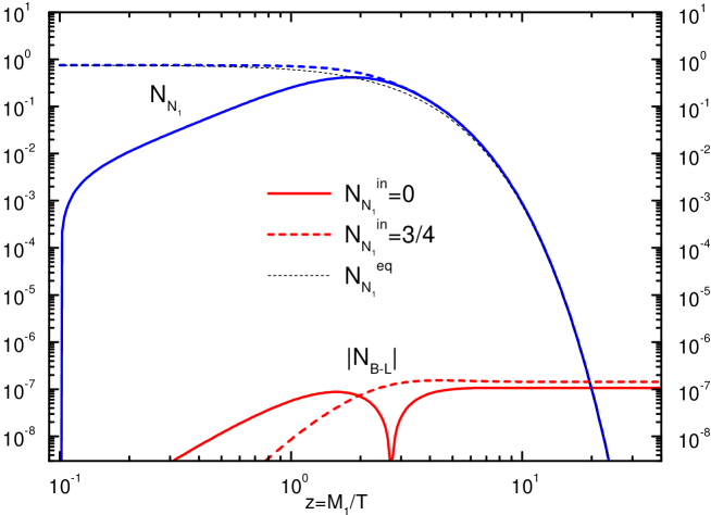
Refer to caption
Figure 1: Evolution of heavy neutrino abundance NN1subscriptNsubscriptN1{\rm N_{N_{1}}} and lepton asymmetry NBLsubscriptNBL{\rm N_{B-L}} for typical leptogenesis parameter: M1=1010GeVsubscript𝑀1superscript1010GeVM_{1}=10^{10}~{}\mathrm{GeV}, m~1=8πΓ1(vew/M1)2=103eVsubscript~𝑚18𝜋subscriptΓ1superscriptsubscript𝑣ewsubscript𝑀12superscript103eV\widetilde{m}_{1}=8\pi\Gamma_{1}(v_{\rm ew}/M_{1})^{2}=10^{-3}~{}\mathrm{eV}, ϵ=106italic-ϵsuperscript106\epsilon=10^{-6}; the inverse temperature z=M1/T𝑧subscript𝑀1𝑇z=M_{1}/T is the time variable. The dashed (full) lines correspond to thermal (vacuum) initial conditions for the heavy neutrino abundance; the dotted line represents the equilibrium abundance. From [30].

In general baryogenesis requires departure from thermal equilibrium. For the cosmological baryon asymmetry, this is provided by the Hubble expansion of the universe and, possibly, also by initial conditions. This can be seen in Fig. 1 where the time evolution of heavy neutrino abundance and lepton asymmetry, as predicted by the Boltzmann equations, are shown for two different initial conditions: thermal and zero heavy neutrino abundance. In the first case, the Hubble expansion leads to an excess of the neutrino abundance at T0.3M1similar-to-or-equals𝑇0.3subscript𝑀1T\simeq 0.3~{}M_{1}; shortly afterwards, washout processes are no longer in equilibrium and the lepton asymmetry is ‘frozen in’. This is the standard out-of-equilibrium decay scenario of baryogenesis. In the second case, interactions with the thermal bath first bring the heavy neutrino into thermal equilibrium; due to the departure from thermal equilibrium during this time, an initial lepton asymmetry is generated. Around T0.3M1similar-to-or-equals𝑇0.3subscript𝑀1T\simeq 0.3~{}M_{1}, this asymmetry is washed out and, as in the first case, the final lepton asymmetry is generated. Remarkably, the initial and the final asymmetry have about the same size. For the generation of the initial asymmetry the change of temperature due to the Hubble expansion is not important. This allows us to make a significant technical simplification in our analysis. Since our goal is the comparison of Boltzmann and Kadanoff-Baym equations, we concentrate on the computation of the initial asymmetry at constant temperature. We expect differences between the classical and the quantum approach to be of similar size in the generation of the final asymmetry. In our numerical analysis we shall consider temperatures T<M<𝑇𝑀T\mathrel{\raise 1.29167pt\hbox{$<$\kern-7.5pt\lower 4.30554pt\hbox{$\sim$}}}M, where the heavy neutrino production rate is not strongly affected by the effect of thermal masses of lepton and Higgs fields [11, 12, 13].

We consider an extension of the Standard Model with additional gauge singlet fermions, i.e., right-handed neutrinos, whose masses and couplings are described by the Lagrangian (sum over i,j𝑖𝑗i,j),

=SM+νR¯ii∂̸νRi+lL¯iϕ~λijνRj+νR¯jλijlLiϕ12Mij(νRc¯iνRj+νR¯jνRic).subscript𝑆𝑀subscript¯subscript𝜈𝑅𝑖𝑖not-partial-differentialsubscript𝜈𝑅𝑖subscript¯subscript𝑙𝐿𝑖~italic-ϕsuperscriptsubscript𝜆𝑖𝑗subscript𝜈𝑅𝑗subscript¯subscript𝜈𝑅𝑗subscript𝜆𝑖𝑗subscript𝑙𝐿𝑖italic-ϕ12subscript𝑀𝑖𝑗subscript¯superscriptsubscript𝜈𝑅𝑐𝑖subscript𝜈𝑅𝑗subscript¯subscript𝜈𝑅𝑗superscriptsubscript𝜈𝑅𝑖𝑐\displaystyle\mathcal{L}=\mathcal{L}_{SM}+\overline{\nu_{R}}_{i}i\displaystyle{\not}{\partial}\nu_{Ri}+\overline{l_{L}}_{i}\tilde{\phi}\lambda_{ij}^{*}\nu_{Rj}+\overline{\nu_{R}}_{j}\lambda_{ij}l_{Li}\phi-\frac{1}{2}M_{ij}\left(\overline{\nu_{R}^{c}}_{i}\nu_{Rj}+\overline{\nu_{R}}_{j}\nu_{Ri}^{c}\right)\ . (1.1)

Here νRc=Cν¯RTsuperscriptsubscript𝜈𝑅𝑐𝐶superscriptsubscript¯𝜈𝑅𝑇\nu_{R}^{c}=C\bar{\nu}_{R}^{T}, C𝐶C is the charge conjugation matrix and ϕ~=iσ2ϕ~italic-ϕ𝑖subscript𝜎2superscriptitalic-ϕ\widetilde{\phi}=i\sigma_{2}\phi^{*}; SU(2) isospin indices have been omitted. For simplicity, we consider the case of hierarchical Majorana masses, Mk>1M1Mmuch-greater-thansubscript𝑀𝑘1subscript𝑀1𝑀M_{k>1}\gg M_{1}\equiv M, and small Yukawa couplings of the lightest heavy neutrino N1Nsubscript𝑁1𝑁N_{1}\equiv N, λi11much-less-thansubscript𝜆𝑖11\lambda_{i1}\ll 1, such that the decay width is much smaller than the mass. Leptogenesis is then dominated by decays and inverse decays of N𝑁N, and it is convenient to integrate out the heavier neutrinos. From Eq. (1.1) one then obtains the effective Lagrangian

=absent\displaystyle\mathcal{L}= SM+12N¯i∂̸N+lL¯iϕ~λi1N+NTλi1ClLiϕ12MNTCNsubscript𝑆𝑀12¯𝑁𝑖not-partial-differential𝑁subscript¯subscript𝑙𝐿𝑖~italic-ϕsuperscriptsubscript𝜆𝑖1𝑁superscript𝑁𝑇subscript𝜆𝑖1𝐶subscript𝑙𝐿𝑖italic-ϕ12𝑀superscript𝑁𝑇𝐶𝑁\displaystyle\mathcal{L}_{SM}+\frac{1}{2}\overline{N}i\displaystyle{\not}{\partial}N+\overline{l_{L}}_{i}\widetilde{\phi}\lambda_{i1}^{*}N+N^{T}\lambda_{i1}Cl_{Li}\phi-\frac{1}{2}MN^{T}CN
+12ηijlLiTϕClLjϕ+12ηijlL¯iϕ~ClL¯jTϕ~,12subscript𝜂𝑖𝑗superscriptsubscript𝑙𝐿𝑖𝑇italic-ϕ𝐶subscript𝑙𝐿𝑗italic-ϕ12superscriptsubscript𝜂𝑖𝑗subscript¯subscript𝑙𝐿𝑖~italic-ϕ𝐶superscriptsubscript¯subscript𝑙𝐿𝑗𝑇~italic-ϕ\displaystyle\;+\frac{1}{2}\eta_{ij}l_{Li}^{T}\phi Cl_{Lj}\phi+\frac{1}{2}\eta_{ij}^{*}\overline{l_{L}}_{i}\widetilde{\phi}C\overline{l_{L}}_{j}^{T}\widetilde{\phi}\ , (1.2)

with N=νR1+νR1c𝑁subscript𝜈𝑅1superscriptsubscript𝜈𝑅1𝑐N=\nu_{R1}+\nu_{R1}^{c}, and the familiar dimension-5 coupling

ηij=k>1λik1MkλkjT.subscript𝜂𝑖𝑗subscript𝑘1subscript𝜆𝑖𝑘1subscript𝑀𝑘superscriptsubscript𝜆𝑘𝑗𝑇\displaystyle\eta_{ij}=\sum_{k>1}\lambda_{ik}\frac{1}{M_{k}}\lambda_{kj}^{T}\ . (1.3)

Using this effective Lagrangian has the advantage that vertex- and self-energy contributions to the CP asymmetry in the heavy neutrino decay [31, 32, 33] are obtained from a single graph [9].

The paper is organized as follows. In Section 2 we present solutions of the Boltzmann equations for the heavy neutrino distribution function and the lepton asymmetry, which are useful for later comparison with the Kadanoff-Baym equations. Some results from nonequilibrium quantum field theory (QFT), in particular equilibrium correlation functions and Kadanoff-Baym equations, are recalled in Section 3. Section 4 contains some of the main results of this paper: analytic solutions of spectral function and statistical propagator for the heavy neutrino. These are needed for the computation of the lepton asymmetry, which is carried out in Section 5. A detailed comparison of the Boltzmann result and the Kadanoff-Baym result is given in Section 6, and numerical results for the generated lepton asymmetries are compared in Section 7. Summary and conclusions are given in Section 8, and various details, including equilibrium correlation functions, Feynman rules, a discussion of the zero-width limit and the computation of some integrals are contained in Appendices A - D.

2 Boltzmann equations

The Boltzmann equations for the time evolution of the distribution functions of heavy neutrinos, lepton and Higgs doublets are well known [34]. As discussed in the previous section, we focus on the generation of the ‘initial asymmetry’ (cf. Fig. 1), which allows us to neglect Hubble expansion and washout terms and to work at constant temperature T𝑇T. The distribution function of the heavy neutrinos is then determined by the first-order differential equation111To simplify notation, we use the same symbol for the modulus of 3-momentum and 4-momentum, e.g., k=|𝐤|𝑘𝐤k=|{\bf k}| and k=(|𝐤|,𝐤)𝑘𝐤𝐤k=(|{\bf k}|,{\bf k}).

tfN(t,ω𝐩)=𝑡subscript𝑓𝑁𝑡subscript𝜔𝐩absent\displaystyle\frac{\partial}{\partial t}f_{N}(t,\omega_{\bf p})= 2ω𝐩𝐤,𝐪(2π)4δ4(k+qp)(λλ)11pk2subscript𝜔𝐩subscript𝐤𝐪superscript2𝜋4superscript𝛿4𝑘𝑞𝑝subscriptsuperscript𝜆𝜆11𝑝𝑘\displaystyle-\frac{2}{\omega_{\bf p}}\int_{\bf k,q}(2\pi)^{4}\delta^{4}(k+q-p)\left(\lambda^{\dagger}\lambda\right)_{11}p\cdot k
×[fN(t,ω𝐩)(1fl(k))(1+fϕ(q))fl(k)fϕ(q)(1fN(t,ω𝐩))],absentdelimited-[]subscript𝑓𝑁𝑡subscript𝜔𝐩1subscript𝑓𝑙𝑘1subscript𝑓italic-ϕ𝑞subscript𝑓𝑙𝑘subscript𝑓italic-ϕ𝑞1subscript𝑓𝑁𝑡subscript𝜔𝐩\displaystyle\times[f_{N}(t,\omega_{\bf p})(1-f_{l}(k))(1+f_{\phi}(q))-f_{l}(k)f_{\phi}(q)(1-f_{N}(t,\omega_{\bf p}))]\ , (2.1)

with vacuum initial condition,

fN(0,ω𝐩)=0;subscript𝑓𝑁0subscript𝜔𝐩0\displaystyle f_{N}(0,\omega_{\bf p})=0\ ; (2.2)

here ω𝐩=M2+𝐩2subscript𝜔𝐩superscript𝑀2superscript𝐩2\omega_{\bf p}=\sqrt{M^{2}+{\bf p}^{2}}, k𝑘k and q𝑞q are the energies of N𝑁N, l𝑙l and ϕitalic-ϕ\phi with equilibrium distribution functions flsubscript𝑓𝑙f_{l} and fϕsubscript𝑓italic-ϕf_{\phi}, respectively; the averaged decay matrix element is |M(N(p)l(k)ϕ(q))|2=2(λλ)11pksuperscript𝑀𝑁𝑝𝑙𝑘italic-ϕ𝑞22subscriptsuperscript𝜆𝜆11𝑝𝑘|M(N(p)\rightarrow l(k)\phi(q))|^{2}=2\left(\lambda^{{\dagger}}\lambda\right)_{11}p\cdot k (cf. [9]). For the momentum integrations we use the notation

𝐩=d3p(2π)32ω.subscript𝐩superscript𝑑3𝑝superscript2𝜋32𝜔\int_{\bf p}\ldots=\int\frac{d^{3}p}{(2\pi)^{3}2\omega}\ldots\ . (2.3)

In most leptogenesis calculations one directly computes the number density,

nN(t)=d3p(2π)3fN(t,ω𝐩),subscript𝑛𝑁𝑡superscript𝑑3𝑝superscript2𝜋3subscript𝑓𝑁𝑡subscript𝜔𝐩\displaystyle n_{N}(t)=\int\frac{d^{3}p}{(2\pi)^{3}}\ f_{N}(t,\omega_{\bf p})\ , (2.4)

assuming kinetic equilibrium.

The sum of decay and inverse decay widths, whose inverse is the time needed to reach thermal equilibrium [35], is given by

Γ𝐩=(λλ)112ω𝐩𝐤,𝐪subscriptΓ𝐩subscriptsuperscript𝜆𝜆112subscript𝜔𝐩subscript𝐤𝐪\displaystyle\Gamma_{\bf p}=\left(\lambda^{\dagger}\lambda\right)_{11}\frac{2}{\omega_{\bf p}}\int_{\bf k,q} (2π)4δ4(k+qp)pkflϕ(k,q),superscript2𝜋4superscript𝛿4𝑘𝑞𝑝𝑝𝑘subscript𝑓𝑙italic-ϕ𝑘𝑞\displaystyle(2\pi)^{4}\delta^{4}(k+q-p)\ p\cdot k\ f_{l\phi}(k,q)\ , (2.5)

where we have introduced the statistical factor (cf. [35])

flϕ(k,q)subscript𝑓𝑙italic-ϕ𝑘𝑞\displaystyle f_{l\phi}(k,q) =fl(k)fϕ(q)+(1fl(k))(1+fϕ(q))absentsubscript𝑓𝑙𝑘subscript𝑓italic-ϕ𝑞1subscript𝑓𝑙𝑘1subscript𝑓italic-ϕ𝑞\displaystyle=f_{l}(k)f_{\phi}(q)+(1-f_{l}(k))(1+f_{\phi}(q))
=1fl(k)+fϕ(q).absent1subscript𝑓𝑙𝑘subscript𝑓italic-ϕ𝑞\displaystyle=1-f_{l}(k)+f_{\phi}(q)\ . (2.6)

Neglecting the momentum dependence of the heavy neutrino width (Γ𝐩ΓsubscriptΓ𝐩Γ\Gamma_{\bf p}\equiv\Gamma), one easily obtains the solution of the Boltzmann equation (2) with vacuum initial condition,

fN(t,ω𝐩)=fNeq(ω𝐩)(1eΓt),subscript𝑓𝑁𝑡subscript𝜔𝐩superscriptsubscript𝑓𝑁𝑒𝑞subscript𝜔𝐩1superscript𝑒Γ𝑡f_{N}(t,\omega_{\bf p})=f_{N}^{eq}(\omega_{\bf p})\left(1-e^{-\Gamma t}\right)\ , (2.7)

where the equilibrium distribution is

fNeq(ω𝐩)=1eβω𝐩+1,superscriptsubscript𝑓𝑁𝑒𝑞subscript𝜔𝐩1superscript𝑒𝛽subscript𝜔𝐩1\displaystyle f_{N}^{eq}(\omega_{\bf p})=\frac{1}{e^{\beta\omega_{\bf p}}+1}\ , (2.8)

and β=1/T𝛽1𝑇\beta=1/T is the inverse temperature.

To compute the lepton asymmetry, we need the Boltzmann equation for the lepton distribution function,

tfl(t,k)=12k𝑡subscript𝑓𝑙𝑡𝑘12𝑘\displaystyle\frac{\partial}{\partial t}f_{l}(t,k)=-\frac{1}{2k} 𝐪,𝐩(2π)4δ4(k+qp)subscript𝐪𝐩superscript2𝜋4superscript𝛿4𝑘𝑞𝑝\displaystyle\int_{\bf q,p}(2\pi)^{4}\delta^{4}(k+q-p)
×\displaystyle\times [|M(lϕN)|2fl(k)fϕ(q)(1fN(t,ω𝐩))\displaystyle\left[|M(l\phi\rightarrow N)|^{2}f_{l}(k)f_{\phi}(q)(1-f_{N}(t,\omega_{\bf p}))\right.
\displaystyle- |M(Nlϕ)|2fN(t,ω𝐩)(1fl(k))(1+fϕ(q))],\displaystyle\left.\ |M(N\rightarrow l\phi)|^{2}f_{N}(t,\omega_{\bf p})(1-f_{l}(k))(1+f_{\phi}(q))\right]\ , (2.9)

where now 𝒪(λ4)𝒪superscript𝜆4\mathcal{O}(\lambda^{4}) corrections to the matrix elements have to be kept. Using Eq. (2.7) one obtains for the lepton asymmetry

fLi(t,k)=fli(t,k)fl¯i(t,k),subscript𝑓𝐿𝑖𝑡𝑘subscript𝑓𝑙𝑖𝑡𝑘subscript𝑓¯𝑙𝑖𝑡𝑘\displaystyle f_{Li}(t,k)=f_{li}(t,k)-f_{\bar{l}i}(t,k)\ , (2.10)

with initial condition fLi(0,k)=0subscript𝑓𝐿𝑖0𝑘0f_{Li}(0,k)=0,

fLi(t,k)=subscript𝑓𝐿𝑖𝑡𝑘\displaystyle f_{Li}(t,k)=- ϵii1k𝐪,𝐩(2π)4δ4(k+qp)pkflϕ(k,q)fNeq(ω𝐩)1Γ(1eΓt),subscriptitalic-ϵ𝑖𝑖1𝑘subscript𝐪𝐩superscript2𝜋4superscript𝛿4𝑘𝑞𝑝𝑝𝑘subscript𝑓𝑙italic-ϕ𝑘𝑞superscriptsubscript𝑓𝑁𝑒𝑞subscript𝜔𝐩1Γ1superscript𝑒Γ𝑡\displaystyle\epsilon_{ii}\frac{1}{k}\int_{\bf q,p}(2\pi)^{4}\delta^{4}(k+q-p)\ p\cdot k\ f_{l\phi}(k,q)f_{N}^{eq}(\omega_{\bf p})\frac{1}{\Gamma}\left(1-e^{-\Gamma t}\right)\ , (2.11)

where we have defined

ϵij=316πIm{λi1(ηλ)j1}M.subscriptitalic-ϵ𝑖𝑗316𝜋Imsubscriptsuperscript𝜆𝑖1subscript𝜂superscript𝜆𝑗1𝑀\displaystyle\epsilon_{ij}=\frac{3}{16\pi}{\rm Im}\{\lambda^{*}_{i1}(\eta\lambda^{*})_{j1}\}M\ . (2.12)

Summing over all lepton flavours, the generated lepton asymmetry is proportional to the familiar CP asymmetry [9],

ϵ=iϵii(λλ)11=316πIm(ληλ)11M(λλ)11.italic-ϵsubscript𝑖subscriptitalic-ϵ𝑖𝑖subscriptsuperscript𝜆𝜆11316𝜋Imsubscriptsuperscript𝜆𝜂superscript𝜆11𝑀subscriptsuperscript𝜆𝜆11\displaystyle\epsilon=\sum_{i}\frac{\epsilon_{ii}}{\left(\lambda^{{\dagger}}\lambda\right)_{11}}=\frac{3}{16\pi}\frac{{\rm Im}\left(\lambda^{{\dagger}}\eta\lambda^{*}\right)_{11}M}{\left(\lambda^{{\dagger}}\lambda\right)_{11}}\ . (2.13)

For later comparison with solutions of the Kadanoff-Baym equations, it is convenient to rewrite Eq. (2.11) as a 4-fold integral,

fLi(t,k)=ϵii16πksubscript𝑓𝐿𝑖𝑡𝑘subscriptitalic-ϵ𝑖𝑖16𝜋𝑘\displaystyle f_{Li}(t,k)=-\epsilon_{ii}\frac{16\pi}{k} 𝐪,𝐩,𝐪,𝐤kk(2π)4δ4(k+qp)(2π)4δ4(k+qp)subscript𝐪𝐩superscript𝐪superscript𝐤𝑘superscript𝑘superscript2𝜋4superscript𝛿4𝑘𝑞𝑝superscript2𝜋4superscript𝛿4superscript𝑘superscript𝑞𝑝\displaystyle\int_{\bf q,p,q^{\prime},k^{\prime}}k\cdot k^{\prime}\ (2\pi)^{4}\delta^{4}(k+q-p)(2\pi)^{4}\delta^{4}(k^{\prime}+q^{\prime}-p)
×flϕ(k,q)fNeq(ω𝐩)1Γ(1eΓt).absentsubscript𝑓𝑙italic-ϕ𝑘𝑞superscriptsubscript𝑓𝑁𝑒𝑞subscript𝜔𝐩1Γ1superscript𝑒Γ𝑡\displaystyle\times f_{l\phi}(k,q)f_{N}^{eq}(\omega_{\bf p})\frac{1}{\Gamma}\left(1-e^{-\Gamma t}\right)\ . (2.14)

The integrand is now proportional to the averaged matrix element |M(lϕl¯ϕ¯)|2=2kk(λλ)11/M2superscript𝑀𝑙italic-ϕ¯𝑙¯italic-ϕ22𝑘superscript𝑘subscriptsuperscript𝜆𝜆11superscript𝑀2|M(l\phi\rightarrow\bar{l}\bar{\phi})|^{2}=2k\cdot k^{\prime}(\lambda^{\dagger}\lambda)_{11}/M^{2} (cf. [9]), which involves the product of the 4-vectors k𝑘k and ksuperscript𝑘k^{\prime}. At low temperatures, TMmuch-less-than𝑇𝑀T\ll M, the integrand falls off like eβω𝐩<eβMsuperscript𝑒𝛽subscript𝜔𝐩superscript𝑒𝛽𝑀e^{-\beta\omega_{\bf p}}<e^{-\beta M}, i.e., the generated asymmetry is strongly suppressed. In standard leptogenesis calculations one considers the integrated lepton asymmetry,

nL=id3k(2π)3fLi(t,k).subscript𝑛𝐿subscript𝑖superscript𝑑3𝑘superscript2𝜋3subscript𝑓𝐿𝑖𝑡𝑘\displaystyle n_{L}=\sum_{i}\int\frac{d^{3}k}{(2\pi)^{3}}\ f_{Li}(t,k)\ . (2.15)

The number densities nNsubscript𝑛𝑁n_{N} (2.4) and nLsubscript𝑛𝐿n_{L} correspond to the comoving number densities NN1subscriptNsubscriptN1{\rm N_{N_{1}}} and |NBL|subscriptNBL{\rm|N_{B-L}|} shown in Fig. 1, in the initial phase of the time evolution, i.e., for T>0.3M>𝑇0.3𝑀T\mathrel{\raise 1.29167pt\hbox{$>$\kern-7.5pt\lower 4.30554pt\hbox{$\sim$}}}0.3\ M.

3 Nonequilibrium QFT and Kadanoff-Baym equations

In the following, we briefly introduce concepts and quantities from nonequilibrium quantum field theory that are necessary for our computation (cf. [36, 37]). A thermodynamical system is represented by a statistical ensemble described by a density matrix ϱitalic-ϱ\varrho. The expectation value for an operator 𝒜𝒜\mathcal{A} is then given by

𝒜=Tr(ϱ𝒜),delimited-⟨⟩𝒜Tritalic-ϱ𝒜\displaystyle\langle\mathcal{A}\rangle={\rm Tr}\left(\varrho\mathcal{A}\right)\ , (3.1)

where we have adopted the usual normalisation Trϱ=1Tritalic-ϱ1{\rm Tr}\varrho=1. Solving the initial value problem for ϱitalic-ϱ\varrho allows to compute all observables for all times. Direct computation of the time evolution of ϱitalic-ϱ\varrho is difficult. Generically, the von Neumann (or quantum Liouville) equation of motion for ϱitalic-ϱ\varrho can only be solved perturbatively for a reduced density matrix with an effective Hamiltonian. In most practical applications to date, a number of additional assumptions are made that lead to effective Boltzmann equations, which can take account of coherent oscillations222See [38, 39] for an application to neutrino oscillations., or quantum corrected Boltzmann equations (cf. Section 6)333In [40, 41] an approach based on first principles has been suggested that is applicable if the occupation numbers for the out-of-equilibrium fields are small..

Instead of the time evolution of the density matrix, one can also directly study the equations of motion of the correlation functions of the theory. The infinitely many degrees of freedom of the initial density matrix are then mapped onto their infinitely many initial conditions. Though a full characterisation of the system in principle involves all n𝑛n-point functions, it is often sufficient to study the one- and two-point function. This applies to the problem considered in this work.

3.1 Correlation functions for lepton and Higgs fields

Leptogenesis occurs at temperatures above the electroweak scale where sphaleron processes are active and transfer the generated lepton asymmetry to a baryon asymmetry. Hence, the Standard Model is in the symmetric phase and the four real degrees of freedom of the Higgs doublet correspond to four massless real scalar fields.

The spectral function and statistical propagator of a real scalar field ϕitalic-ϕ\phi, ΔsuperscriptΔ\Delta^{-} and Δ+superscriptΔ\Delta^{+}, respectively, are defined as

Δ(x1,x2)superscriptΔsubscript𝑥1subscript𝑥2\displaystyle\Delta^{-}(x_{1},x_{2}) =i[ϕ(x1),ϕ(x2)],absent𝑖delimited-⟨⟩italic-ϕsubscript𝑥1italic-ϕsubscript𝑥2\displaystyle=i\langle[\phi(x_{1}),\phi(x_{2})]\rangle\ , (3.2)
Δ+(x1,x2)superscriptΔsubscript𝑥1subscript𝑥2\displaystyle\Delta^{+}(x_{1},x_{2}) =12{ϕ(x1),ϕ(x2)}.absent12delimited-⟨⟩italic-ϕsubscript𝑥1italic-ϕsubscript𝑥2\displaystyle=\frac{1}{2}\langle\{\phi(x_{1}),\phi(x_{2})\}\rangle\ . (3.3)

Here only contributions from connected diagrams are to be included to compute the dressed correlation functions. These fulfill the symmetry relations

Δ(x1,x2)superscriptΔsubscript𝑥1subscript𝑥2\displaystyle\Delta^{-}(x_{1},x_{2}) =Δ(x2,x1),absentsuperscriptΔsubscript𝑥2subscript𝑥1\displaystyle=-\Delta^{-}(x_{2},x_{1})\ , (3.4)
Δ+(x1,x2)superscriptΔsubscript𝑥1subscript𝑥2\displaystyle\Delta^{+}(x_{1},x_{2}) =Δ+(x2,x1),absentsuperscriptΔsubscript𝑥2subscript𝑥1\displaystyle=\Delta^{+}(x_{2},x_{1})\ , (3.5)

which follow directly from the definitions.

The functions Δ±superscriptΔplus-or-minus\Delta^{\pm} have an intuitive physical interpretation. The spectral function ΔsuperscriptΔ\Delta^{-} is the Fourier transform of the spectral density,

ρq(t,ω)=idy2πeiωyΔ(t+y2,ty2),subscript𝜌q𝑡𝜔𝑖𝑑𝑦2𝜋superscript𝑒𝑖𝜔𝑦superscriptΔ𝑡𝑦2𝑡𝑦2\displaystyle\rho_{\textbf{q}}(t,\omega)=-i\int\frac{dy}{2\pi}e^{i\omega y}\Delta^{-}(t+\frac{y}{2},t-\frac{y}{2})\ , (3.6)

where we have used the relative and total time coordinates, y=t1t2𝑦subscript𝑡1subscript𝑡2y=t_{1}-t_{2} and t=(t1+t2)/2𝑡subscript𝑡1subscript𝑡22t=(t_{1}+t_{2})/2, respectively.

The spectral density ρq(t,ω)subscript𝜌q𝑡𝜔\rho_{\textbf{q}}(t,\omega) characterises the density of quantum mechanical states in phase space. Propagating states, or resonances, appear as peaks in the spectral function. The statistical propagator contains the information about the occupation number of each state.

In the following we shall also need the Wightman functions

Δ>(x1,x2)superscriptΔsubscript𝑥1subscript𝑥2\displaystyle\Delta^{>}(x_{1},x_{2}) =ϕ(x1)ϕ(x2),absentdelimited-⟨⟩italic-ϕsubscript𝑥1italic-ϕsubscript𝑥2\displaystyle=\langle\phi(x_{1})\phi(x_{2})\rangle\ , (3.7)
Δ<(x1,x2)superscriptΔsubscript𝑥1subscript𝑥2\displaystyle\Delta^{<}(x_{1},x_{2}) =ϕ(x2)ϕ(x1),absentdelimited-⟨⟩italic-ϕsubscript𝑥2italic-ϕsubscript𝑥1\displaystyle=\langle\phi(x_{2})\phi(x_{1})\rangle\ , (3.8)

which are related to Δ±superscriptΔplus-or-minus\Delta^{\pm} by

Δ(x1,x2)superscriptΔsubscript𝑥1subscript𝑥2\displaystyle\Delta^{-}(x_{1},x_{2}) =i(Δ>(x1,x2)Δ<(x1,x2)),absent𝑖superscriptΔsubscript𝑥1subscript𝑥2superscriptΔsubscript𝑥1subscript𝑥2\displaystyle=i\left(\Delta^{>}(x_{1},x_{2})-\Delta^{<}(x_{1},x_{2})\right)\ , (3.9)
Δ+(x1,x2)superscriptΔsubscript𝑥1subscript𝑥2\displaystyle\Delta^{+}(x_{1},x_{2}) =12(Δ>(x1,x2)+Δ<(x1,x2)).absent12superscriptΔsubscript𝑥1subscript𝑥2superscriptΔsubscript𝑥1subscript𝑥2\displaystyle=\frac{1}{2}\left(\Delta^{>}(x_{1},x_{2})+\Delta^{<}(x_{1},x_{2})\right)\ . (3.10)

Using microcausality and the condition for canonical quantization,

[ϕ(x1),ϕ(x2)]|t1=t2evaluated-atitalic-ϕsubscript𝑥1italic-ϕsubscript𝑥2subscript𝑡1subscript𝑡2\displaystyle[\phi(x_{1}),\phi(x_{2})]|_{t_{1}=t_{2}} =[ϕ˙(x1),ϕ˙(x2)]|t1=t2=0,absentevaluated-at˙italic-ϕsubscript𝑥1˙italic-ϕsubscript𝑥2subscript𝑡1subscript𝑡20\displaystyle=[\dot{\phi}(x_{1}),\dot{\phi}(x_{2})]|_{t_{1}=t_{2}}=0\ , (3.11)
[ϕ(x1),ϕ˙(x2)]|t1=t2evaluated-atitalic-ϕsubscript𝑥1˙italic-ϕsubscript𝑥2subscript𝑡1subscript𝑡2\displaystyle[\phi(x_{1}),\dot{\phi}(x_{2})]|_{t_{1}=t_{2}} =iδ(𝐱1𝐱2),absent𝑖𝛿subscript𝐱1subscript𝐱2\displaystyle=i\delta({\bf x}_{1}-{\bf x}_{2})\ , (3.12)

one obtains boundary conditions in y=t1t2𝑦subscript𝑡1subscript𝑡2y=t_{1}-t_{2} for ΔsuperscriptΔ\Delta^{-},

Δ(x1,x2)|t1=t2evaluated-atsuperscriptΔsubscript𝑥1subscript𝑥2subscript𝑡1subscript𝑡2\displaystyle\Delta^{-}(x_{1},x_{2})|_{t_{1}=t_{2}} =0,absent0\displaystyle=0\ , (3.13)
t1Δ(x1,x2)|t1=t2evaluated-atsubscriptsubscript𝑡1superscriptΔsubscript𝑥1subscript𝑥2subscript𝑡1subscript𝑡2\displaystyle\partial_{t_{1}}\Delta^{-}(x_{1},x_{2})|_{t_{1}=t_{2}} =t2Δ(x1,x2)|t1=t2=δ(𝐱1𝐱2),absentevaluated-atsubscriptsubscript𝑡2superscriptΔsubscript𝑥1subscript𝑥2subscript𝑡1subscript𝑡2𝛿subscript𝐱1subscript𝐱2\displaystyle=-\partial_{t_{2}}\Delta^{-}(x_{1},x_{2})|_{t_{1}=t_{2}}=\delta({\bf x}_{1}-{\bf x}_{2})\ , (3.14)
t1t2Δ(x1,x2)|t1=t2evaluated-atsubscriptsubscript𝑡1subscriptsubscript𝑡2superscriptΔsubscript𝑥1subscript𝑥2subscript𝑡1subscript𝑡2\displaystyle\partial_{t_{1}}\partial_{t_{2}}\Delta^{-}(x_{1},x_{2})|_{t_{1}=t_{2}} =0.absent0\displaystyle=0\ . (3.15)

Note that these conditions do not depend on the physical initial conditions of the system encoded in the initial density matrix. These enter via the initial conditions for the statistical propagator.

Analogous to Δ±superscriptΔplus-or-minus\Delta^{\pm}, one can define the spectral functions and statistical propagators for fermions. The fermionic fields in the Lagrangian (1) are massless left-handed leptons (Weyl fields lLisubscript𝑙𝐿𝑖l_{Li}) and a massive neutrino (Majorana field N𝑁N). For the massless leptons, spectral function and statistical propagator are defined as

(SLij)αβ(x1,x2)subscriptsubscriptsuperscript𝑆𝐿𝑖𝑗𝛼𝛽subscript𝑥1subscript𝑥2\displaystyle(S^{-}_{Lij})_{\alpha\beta}(x_{1},x_{2}) =i{lLiα(x1),l¯Ljβ(x2)},absent𝑖delimited-⟨⟩subscript𝑙𝐿𝑖𝛼subscript𝑥1subscript¯𝑙𝐿𝑗𝛽subscript𝑥2\displaystyle=i\langle\{l_{Li\alpha}(x_{1}),\bar{l}_{Lj\beta}(x_{2})\}\rangle\ , (3.16)
(SLij+)αβ(x1,x2)subscriptsubscriptsuperscript𝑆𝐿𝑖𝑗𝛼𝛽subscript𝑥1subscript𝑥2\displaystyle(S^{+}_{Lij})_{\alpha\beta}(x_{1},x_{2}) =12[lLiα(x1),l¯Ljβ(x2)],absent12delimited-⟨⟩subscript𝑙𝐿𝑖𝛼subscript𝑥1subscript¯𝑙𝐿𝑗𝛽subscript𝑥2\displaystyle={1\over 2}\langle[l_{Li\alpha}(x_{1}),\bar{l}_{Lj\beta}(x_{2})]\rangle\ , (3.17)

where α𝛼\alpha and β𝛽\beta are spinor indices, and SU(2) indices were omitted for notational simplicity. The subscript L𝐿L denotes the projection to left-handed fields, i.e., SL±=PLS±subscriptsuperscript𝑆plus-or-minus𝐿subscript𝑃𝐿superscript𝑆plus-or-minusS^{\pm}_{L}=P_{L}S^{\pm}, where PL=(1γ5)/2subscript𝑃𝐿1superscript𝛾52P_{L}=(1-\gamma^{5})/2 and S±superscript𝑆plus-or-minusS^{\pm} are the propagators for Dirac fermions. As for bosons, we shall need the functions

(SLij>)αβ(x1,x2)subscriptsubscriptsuperscript𝑆𝐿𝑖𝑗𝛼𝛽subscript𝑥1subscript𝑥2\displaystyle(S^{>}_{Lij})_{\alpha\beta}(x_{1},x_{2}) =lLiα(x1)l¯Ljβ(x2),absentdelimited-⟨⟩subscript𝑙𝐿𝑖𝛼subscript𝑥1subscript¯𝑙𝐿𝑗𝛽subscript𝑥2\displaystyle=\langle l_{Li\alpha}(x_{1})\bar{l}_{Lj\beta}(x_{2})\rangle\ , (3.18)
(SLij<)αβ(x1,x2)subscriptsubscriptsuperscript𝑆𝐿𝑖𝑗𝛼𝛽subscript𝑥1subscript𝑥2\displaystyle(S^{<}_{Lij})_{\alpha\beta}(x_{1},x_{2}) =l¯Ljβ(x2)lLiα(x1),absentdelimited-⟨⟩subscript¯𝑙𝐿𝑗𝛽subscript𝑥2subscript𝑙𝐿𝑖𝛼subscript𝑥1\displaystyle=-\langle\bar{l}_{Lj\beta}(x_{2})l_{Li\alpha}(x_{1})\rangle\ , (3.19)

which are related to spectral function and statistical propagator by

SLij(x1,x2)subscriptsuperscript𝑆𝐿𝑖𝑗subscript𝑥1subscript𝑥2\displaystyle S^{-}_{Lij}(x_{1},x_{2}) =i(SLij>(x1,x2)SLij<(x1,x2)),absent𝑖subscriptsuperscript𝑆𝐿𝑖𝑗subscript𝑥1subscript𝑥2subscriptsuperscript𝑆𝐿𝑖𝑗subscript𝑥1subscript𝑥2\displaystyle=i\left(S^{>}_{Lij}(x_{1},x_{2})-S^{<}_{Lij}(x_{1},x_{2})\right)\ , (3.20)
SLij+(x1,x2)subscriptsuperscript𝑆𝐿𝑖𝑗subscript𝑥1subscript𝑥2\displaystyle S^{+}_{Lij}(x_{1},x_{2}) =12(SLij>(x1,x2)+SLij<(x1,x2)).absent12subscriptsuperscript𝑆𝐿𝑖𝑗subscript𝑥1subscript𝑥2subscriptsuperscript𝑆𝐿𝑖𝑗subscript𝑥1subscript𝑥2\displaystyle=\frac{1}{2}\left(S^{>}_{Lij}(x_{1},x_{2})+S^{<}_{Lij}(x_{1},x_{2})\right)\ . (3.21)

The propagators S±superscript𝑆plus-or-minusS^{\pm} have the symmetry properties

γ0[SLij(x1,x2)]γ0subscript𝛾0superscriptdelimited-[]subscriptsuperscript𝑆𝐿𝑖𝑗subscript𝑥1subscript𝑥2subscript𝛾0\displaystyle\gamma_{0}\left[S^{-}_{Lij}(x_{1},x_{2})\right]^{\dagger}\gamma_{0} =SLji(x2,x1),absentsubscriptsuperscript𝑆𝐿𝑗𝑖subscript𝑥2subscript𝑥1\displaystyle=-S^{-}_{Lji}(x_{2},x_{1})\ , (3.22)
γ0[SLij+(x1,x2)]γ0subscript𝛾0superscriptdelimited-[]subscriptsuperscript𝑆𝐿𝑖𝑗subscript𝑥1subscript𝑥2subscript𝛾0\displaystyle\gamma_{0}\left[S^{+}_{Lij}(x_{1},x_{2})\right]^{\dagger}\gamma_{0} =SLji+(x2,x1).absentsubscriptsuperscript𝑆𝐿𝑗𝑖subscript𝑥2subscript𝑥1\displaystyle=S^{+}_{Lji}(x_{2},x_{1})\ . (3.23)

The canonical quantization condition,

{lLiα(x1),lLjβ(x2)}=PLαβδijδ(𝐱1𝐱2),subscript𝑙𝐿𝑖𝛼subscript𝑥1subscriptsuperscript𝑙𝐿𝑗𝛽subscript𝑥2subscript𝑃𝐿𝛼𝛽subscript𝛿𝑖𝑗𝛿subscript𝐱1subscript𝐱2\displaystyle\{l_{Li\alpha}(x_{1}),l^{\dagger}_{Lj\beta}(x_{2})\}=P_{L\alpha\beta}\delta_{ij}\delta({\bf x}_{1}-{\bf x}_{2})\ , (3.24)

implies the boundary condition for the spectral function

SLij(x1,x2)|t1=t2=iPLδijδ(𝐱1𝐱2).evaluated-atsuperscriptsubscript𝑆𝐿𝑖𝑗subscript𝑥1subscript𝑥2subscript𝑡1subscript𝑡2𝑖subscript𝑃𝐿subscript𝛿𝑖𝑗𝛿subscript𝐱1subscript𝐱2\displaystyle S_{Lij}^{-}(x_{1},x_{2})|_{t_{1}=t_{2}}=iP_{L}\delta_{ij}\delta({\bf x}_{1}-{\bf x}_{2})\ . (3.25)

Finally, spectral function and statistical propagator for the Majorana field N𝑁N read

Gαβ(x1,x2)subscriptsuperscript𝐺𝛼𝛽subscript𝑥1subscript𝑥2\displaystyle G^{-}_{\alpha\beta}(x_{1},x_{2}) =i{Nα(x1),Nβ(x2)},absent𝑖delimited-⟨⟩subscript𝑁𝛼subscript𝑥1subscript𝑁𝛽subscript𝑥2\displaystyle=i\langle\{N_{\alpha}(x_{1}),N_{\beta}(x_{2})\}\rangle\ , (3.26)
Gαβ+(x1,x2)subscriptsuperscript𝐺𝛼𝛽subscript𝑥1subscript𝑥2\displaystyle G^{+}_{\alpha\beta}(x_{1},x_{2}) =12[Nα(x1),Nβ(x2)].absent12delimited-⟨⟩subscript𝑁𝛼subscript𝑥1subscript𝑁𝛽subscript𝑥2\displaystyle={1\over 2}\langle[N_{\alpha}(x_{1}),N_{\beta}(x_{2})]\rangle\ . (3.27)

They have the symmetries

G(x1,x2)superscript𝐺subscript𝑥1subscript𝑥2\displaystyle G^{-}(x_{1},x_{2}) =G(x2,x1)T,absentsuperscript𝐺superscriptsubscript𝑥2subscript𝑥1𝑇\displaystyle=G^{-}(x_{2},x_{1})^{T}\ , (3.28)
G+(x1,x2)superscript𝐺subscript𝑥1subscript𝑥2\displaystyle G^{+}(x_{1},x_{2}) =G+(x2,x1)T.absentsuperscript𝐺superscriptsubscript𝑥2subscript𝑥1𝑇\displaystyle=-G^{+}(x_{2},x_{1})^{T}\ . (3.29)

The canonical quantization condition, together with the Majorana property N=CN¯T𝑁𝐶superscript¯𝑁𝑇N=C\bar{N}^{T}, implies the boundary condition

G(x1,x2)|t1=t2=iγ0δ(𝐱1𝐱2)C1.evaluated-atsuperscript𝐺subscript𝑥1subscript𝑥2subscript𝑡1subscript𝑡2𝑖superscript𝛾0𝛿subscript𝐱1subscript𝐱2superscript𝐶1\displaystyle G^{-}(x_{1},x_{2})|_{t_{1}=t_{2}}=i\gamma^{0}\delta({\bf x}_{1}-{\bf x}_{2})C^{-1}\ . (3.30)

As for scalars, the physical initial conditions enter as boundary conditions for the statistical propagator. In the following, we will consider two types of initial conditions, thermal equilibrium and Gaussian initial correlations, for which we solve the equations of motion in the following section. Analogous to real scalars, the functions Gsuperscript𝐺greater-than-or-less-thanG^{\gtrless} are defined as

Gαβ>(x1,x2)subscriptsuperscript𝐺𝛼𝛽subscript𝑥1subscript𝑥2\displaystyle G^{>}_{\alpha\beta}(x_{1},x_{2}) =Nα(x1)Nβ(x2),absentdelimited-⟨⟩subscript𝑁𝛼subscript𝑥1subscript𝑁𝛽subscript𝑥2\displaystyle=\langle N_{\alpha}(x_{1})N_{\beta}(x_{2})\rangle\ , (3.31)
Gαβ<(x1,x2)subscriptsuperscript𝐺𝛼𝛽subscript𝑥1subscript𝑥2\displaystyle G^{<}_{\alpha\beta}(x_{1},x_{2}) =Nβ(x2)Nα(x1),absentdelimited-⟨⟩subscript𝑁𝛽subscript𝑥2subscript𝑁𝛼subscript𝑥1\displaystyle=-\langle N_{\beta}(x_{2})N_{\alpha}(x_{1})\rangle, (3.32)

with the usual relations to spectral function and statistical propagator,

G(x1,x2)superscript𝐺subscript𝑥1subscript𝑥2\displaystyle G^{-}(x_{1},x_{2}) =i(G>(x1,x2)G<(x1,x2)),absent𝑖superscript𝐺subscript𝑥1subscript𝑥2superscript𝐺subscript𝑥1subscript𝑥2\displaystyle=i\left(G^{>}(x_{1},x_{2})-G^{<}(x_{1},x_{2})\right)\ , (3.33)
G+(x1,x2)superscript𝐺subscript𝑥1subscript𝑥2\displaystyle G^{+}(x_{1},x_{2}) =12(G>(x1,x2)+G<(x1,x2)).absent12superscript𝐺subscript𝑥1subscript𝑥2superscript𝐺subscript𝑥1subscript𝑥2\displaystyle=\frac{1}{2}\left(G^{>}(x_{1},x_{2})+G^{<}(x_{1},x_{2})\right)\ . (3.34)

3.2 Equations of motion

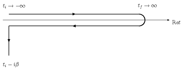
In thermal leptogenesis, the deviation from thermal equilibrium that is necessary to create a matter-antimatter asymmetry is due to the heavy Majorana neutrinos which are out of equilibrium. The equations of motion for their correlation functions G±superscript𝐺plus-or-minusG^{\pm} can be obtained via the Schwinger-Keldysh formalism [6]. The basic quantity is the Green’s function with time arguments defined on a contour 𝒞𝒞\mathcal{C} in the complex x0superscript𝑥0x^{0}-plane, known as the Keldysh contour (cf. Fig.2),

G𝒞(x1,x2)=θ𝒞(x10,x20)G>(x1,x2)+θ𝒞(x20,x10)G<(x1,x2).subscript𝐺𝒞subscript𝑥1subscript𝑥2subscript𝜃𝒞subscriptsuperscript𝑥01subscriptsuperscript𝑥02superscript𝐺subscript𝑥1subscript𝑥2subscript𝜃𝒞subscriptsuperscript𝑥02subscriptsuperscript𝑥01superscript𝐺subscript𝑥1subscript𝑥2G_{\mathcal{C}}(x_{1},x_{2})=\theta_{\mathcal{C}}(x^{0}_{1},x^{0}_{2})G^{>}(x_{1},x_{2})+\theta_{\mathcal{C}}(x^{0}_{2},x^{0}_{1})G^{<}(x_{1},x_{2})\ . (3.35)

Here the θ𝜃\theta-functions enforce path ordering along the contour 𝒞𝒞\mathcal{C}.

Refer to caption
Figure 2: Path in the complex time plane for nonequilibrium Green’s functions. The contour runs from some initial time x0=ti+iϵsuperscript𝑥0subscript𝑡𝑖𝑖italic-ϵx^{0}=t_{i}+i\epsilon (ti=0)t_{i}=0) parallel to the real axis (x0=t+iϵsuperscript𝑥0𝑡𝑖italic-ϵx^{0}=t+i\epsilon) up to some final time tf+iϵsubscript𝑡𝑓𝑖italic-ϵt_{f}+i\epsilon and returns to tiiϵsubscript𝑡𝑖𝑖italic-ϵt_{i}-i\epsilon. To compute physical correlation functions for arbitrary times t>ti𝑡subscript𝑡𝑖t>t_{i}, one takes the limits tfsubscript𝑡𝑓t_{f}\rightarrow\infty and ϵ0italic-ϵ0\epsilon\rightarrow 0.

The necessity of considering Green’s functions with time arguments on the Keldysh contour (rather than the real axis) is a consequence of the fact that nonequilibrium processes are initial value problems. The system is prepared at initial time tisubscript𝑡𝑖t_{i}, its state at later times is unknown. Hence, the usual approach to define a S-matrix by projection onto asymptotic ‘in’ and ‘out’ states, sending initial and final time to infinity, cannot be applied. When using the Keldysh contour which starts and ends at the same time tisubscript𝑡𝑖t_{i}444Due to this fact this formalism is sometimes called ‘in-in’ formalism, in contrast to the ‘in-out’ formalism used to compute the S-matrix., no knowledge of the system’s state at t=±𝑡plus-or-minust=\pm\infty is needed to define a generating functional for correlation functions.

The Green’s function G𝒞subscript𝐺𝒞G_{\mathcal{C}} satisfies the Schwinger-Dyson equation

C(i∂̸1M)G𝒞(x1,x2)i𝒞d4xCΣ𝒞(x1,x)G𝒞(x,x2)=iδ𝒞(x1x2),𝐶𝑖subscriptnot-partial-differential1𝑀subscript𝐺𝒞subscript𝑥1subscript𝑥2𝑖subscript𝒞superscript𝑑4superscript𝑥𝐶subscriptΣ𝒞subscript𝑥1superscript𝑥subscript𝐺𝒞superscript𝑥subscript𝑥2𝑖subscript𝛿𝒞subscript𝑥1subscript𝑥2\displaystyle C(i\displaystyle{\not}{\partial}_{1}-M)G_{\mathcal{C}}(x_{1},x_{2})-i\int_{\mathcal{C}}d^{4}x^{\prime}C\Sigma_{\mathcal{C}}(x_{1},x^{\prime})G_{\mathcal{C}}(x^{\prime},x_{2})=i\delta_{\mathcal{C}}(x_{1}-x_{2})\ , (3.36)

where CΣ𝒞(x1,x)𝐶subscriptΣ𝒞subscript𝑥1superscript𝑥C\Sigma_{\mathcal{C}}(x_{1},x^{\prime}) is the self-energy555An explicit factor C𝐶C is factorized for later convenience. on the contour and ∂̸1=γμ/x1μsubscriptnot-partial-differential1superscript𝛾𝜇superscriptsubscript𝑥1𝜇\displaystyle{\not}{\partial}_{1}=\gamma^{\mu}\partial/\partial x_{1}^{\mu}. Like the Green’s function, also the self-energy can be decomposed as

Σ𝒞(x1,x2)=θ𝒞(x10,x20)Σ>(x1,x2)+θ𝒞(x20,x10)Σ<(x1,x2).subscriptΣ𝒞subscript𝑥1subscript𝑥2subscript𝜃𝒞subscriptsuperscript𝑥01subscriptsuperscript𝑥02superscriptΣsubscript𝑥1subscript𝑥2subscript𝜃𝒞subscriptsuperscript𝑥02subscriptsuperscript𝑥01superscriptΣsubscript𝑥1subscript𝑥2\displaystyle\Sigma_{\mathcal{C}}(x_{1},x_{2})=\theta_{\mathcal{C}}(x^{0}_{1},x^{0}_{2})\Sigma^{>}(x_{1},x_{2})+\theta_{\mathcal{C}}(x^{0}_{2},x^{0}_{1})\Sigma^{<}(x_{1},x_{2})\ . (3.37)

In the Schwinger-Dyson equation (3.36) the time coordinates of G𝒞subscript𝐺𝒞G_{\mathcal{C}} and Σ𝒞subscriptΣ𝒞\Sigma_{\mathcal{C}} can lie on the upper or the lower branch of the contour.

The familar time-ordered Feynman propagator is obtained from G𝒞(x1,x2)subscript𝐺𝒞subscript𝑥1subscript𝑥2G_{\mathcal{C}}(x_{1},x_{2}) when both time arguments lie on the upper branch, and therefore denoted by G11superscript𝐺11G^{11}. Correspondingly, G𝒞(x1,x2)subscript𝐺𝒞subscript𝑥1subscript𝑥2G_{\mathcal{C}}(x_{1},x_{2}) with both time arguments on the lower part of the contour corresponds to an anti-time-ordered propagator, denoted as G22superscript𝐺22G^{22}. For correlators with one time argument on the upper and one on the lower part of the contour, referred to as G12superscript𝐺12G^{12} and G21superscript𝐺21G^{21}, the order of field operators is fixed by the path ordering: operators on the upper branch are always ‘earlier’ than those on the lower branch (cf. 3.35). Altogether, one has

G12(x1,x2)superscript𝐺12subscript𝑥1subscript𝑥2\displaystyle G^{12}(x_{1},x_{2}) =G<(x1,x2),absentsuperscript𝐺subscript𝑥1subscript𝑥2\displaystyle=G^{<}(x_{1},x_{2})\ , (3.38)
G21(x1,x2)superscript𝐺21subscript𝑥1subscript𝑥2\displaystyle G^{21}(x_{1},x_{2}) =G>(x1,x2),absentsuperscript𝐺subscript𝑥1subscript𝑥2\displaystyle=G^{>}(x_{1},x_{2})\ , (3.39)
G11(x1,x2)superscript𝐺11subscript𝑥1subscript𝑥2\displaystyle G^{11}(x_{1},x_{2}) =G+(x1,x2)i2sign(x10x20)G(x1,x2),absentsuperscript𝐺subscript𝑥1subscript𝑥2𝑖2signsubscriptsuperscript𝑥01subscriptsuperscript𝑥02superscript𝐺subscript𝑥1subscript𝑥2\displaystyle=G^{+}(x_{1},x_{2})-\frac{i}{2}{\rm sign}(x^{0}_{1}-x^{0}_{2})G^{-}(x_{1},x_{2})\ , (3.40)
G22(x1,x2)superscript𝐺22subscript𝑥1subscript𝑥2\displaystyle G^{22}(x_{1},x_{2}) =G+(x1,x2)+i2sign(x10x20)G(x1,x2);absentsuperscript𝐺subscript𝑥1subscript𝑥2𝑖2signsubscriptsuperscript𝑥01subscriptsuperscript𝑥02superscript𝐺subscript𝑥1subscript𝑥2\displaystyle=G^{+}(x_{1},x_{2})+\frac{i}{2}{\rm sign}(x^{0}_{1}-x^{0}_{2})G^{-}(x_{1},x_{2})\ ; (3.41)

the last two relations are easily verified by inserting the definitions of G±superscript𝐺plus-or-minusG^{\pm}.

In a perturbative expansion of the Schwinger-Dyson equation (3.36) in terms of Feynman diagrams, time arguments of internal vertices can lie on either branch. Hence, the number of contributing graphs doubles with each internal vertex since this can lie on the upper or the lower branch666This fact is sometimes referred to as ‘doubling of degrees of freedom’.. Two upper vertices are connected by G11superscript𝐺11G^{11}, two lower vertices by G22superscript𝐺22G^{22} and vertices of different type by G12superscript𝐺12G^{12} and G21superscript𝐺21G^{21}. Each lower vertex leads to an additional factor 11-1.

Like the Green’s function, also the self-energy Σ𝒞subscriptΣ𝒞\Sigma_{\mathcal{C}}, the sum of all one-particle irreducible graphs, can be dissected into components ΣklsuperscriptΣ𝑘𝑙\Sigma^{kl}, with k𝑘k and l𝑙l being ‘contour indices’ as defined above. Analogous to (3.38) and (3.39) one then defines self-energies ΣsuperscriptΣgreater-than-or-less-than\Sigma^{\gtrless} and, following (3.33) and (3.34), self-energies Σ±superscriptΣplus-or-minus\Sigma^{\pm} via the equations

Σ(x1,x2)superscriptΣsubscript𝑥1subscript𝑥2\displaystyle\Sigma^{-}(x_{1},x_{2}) =i(Σ>(x1,x2)Σ<(x1,x2)),absent𝑖superscriptΣsubscript𝑥1subscript𝑥2superscriptΣsubscript𝑥1subscript𝑥2\displaystyle=i\left(\Sigma^{>}(x_{1},x_{2})-\Sigma^{<}(x_{1},x_{2})\right)\ , (3.42)
Σ+(x1,x2)superscriptΣsubscript𝑥1subscript𝑥2\displaystyle\Sigma^{+}(x_{1},x_{2}) =12(Σ>(x1,x2)+Σ<(x1,x2)).absent12superscriptΣsubscript𝑥1subscript𝑥2superscriptΣsubscript𝑥1subscript𝑥2\displaystyle=\frac{1}{2}\left(\Sigma^{>}(x_{1},x_{2})+\Sigma^{<}(x_{1},x_{2})\right)\ . (3.43)

Since the self-energies ΣklsuperscriptΣ𝑘𝑙\Sigma^{kl} are directly related to the full Green’s functions Gklsuperscript𝐺𝑘𝑙G^{kl}, they also satisfy the relations (3.38) - (3.41).

Using the above relations for Gklsuperscript𝐺𝑘𝑙G^{kl} and ΣklsuperscriptΣ𝑘𝑙\Sigma^{kl}, one obtains, after a straightforward calculation, from the Schwinger-Dyson equation (3.36) a system of two coupled differential equations for G𝐩±subscriptsuperscript𝐺plus-or-minus𝐩G^{\pm}_{\bf p}, the Kadanoff-Baym equations. Due to spatial homogeneity, we can consider the equations for each Fourier mode separately,

C(iγ0t1𝐩𝜸M)G𝐩(t1,t2)=𝐶𝑖superscript𝛾0subscriptsubscript𝑡1𝐩𝜸𝑀superscriptsubscript𝐺𝐩subscript𝑡1subscript𝑡2absent\displaystyle C(i\gamma^{0}\partial_{t_{1}}-{\bf p}\boldsymbol{\gamma}-M)G_{\bf p}^{-}(t_{1},t_{2})= t1t2𝑑tCΣ𝐩(t1,t)G𝐩(t,t2),superscriptsubscriptsubscript𝑡1subscript𝑡2differential-dsuperscript𝑡𝐶superscriptsubscriptΣ𝐩subscript𝑡1superscript𝑡superscriptsubscript𝐺𝐩superscript𝑡subscript𝑡2\displaystyle-\int_{t_{1}}^{t_{2}}dt^{\prime}C\Sigma_{\bf p}^{-}(t_{1},t^{\prime})G_{\bf p}^{-}(t^{\prime},t_{2})\ , (3.44)
C(iγ0t1𝐩𝜸M)G𝐩+(t1,t2)=𝐶𝑖superscript𝛾0subscriptsubscript𝑡1𝐩𝜸𝑀superscriptsubscript𝐺𝐩subscript𝑡1subscript𝑡2absent\displaystyle C(i\gamma^{0}\partial_{t_{1}}-{\bf p}\boldsymbol{\gamma}-M)G_{\bf p}^{+}(t_{1},t_{2})= tit2𝑑tCΣ𝐩+(t1,t)G𝐩(t,t2)subscriptsuperscriptsubscript𝑡2subscript𝑡𝑖differential-dsuperscript𝑡𝐶superscriptsubscriptΣ𝐩subscript𝑡1superscript𝑡superscriptsubscript𝐺𝐩superscript𝑡subscript𝑡2\displaystyle-\int^{t_{2}}_{t_{i}}dt^{\prime}C\Sigma_{\bf p}^{+}(t_{1},t^{\prime})G_{\bf p}^{-}(t^{\prime},t_{2})
+tit1𝑑tCΣ𝐩(t1,t)G𝐩+(t,t2).subscriptsuperscriptsubscript𝑡1subscript𝑡𝑖differential-dsuperscript𝑡𝐶subscriptsuperscriptΣ𝐩subscript𝑡1superscript𝑡superscriptsubscript𝐺𝐩superscript𝑡subscript𝑡2\displaystyle+\int^{t_{1}}_{t_{i}}dt^{\prime}C\Sigma^{-}_{\bf p}(t_{1},t^{\prime})G_{\bf p}^{+}(t^{\prime},t_{2})\ . (3.45)

For the lepton propagators SL𝐤±subscriptsuperscript𝑆plus-or-minus𝐿𝐤S^{\pm}_{L{\bf k}} one obtains the same equations, with CΣ𝐩±𝐶superscriptsubscriptΣ𝐩plus-or-minusC\Sigma_{\bf p}^{\pm} replaced by the lepton self-energies Π𝐤±superscriptsubscriptΠ𝐤plus-or-minus\Pi_{\bf k}^{\pm} and no charge conjugation matrix C multiplying the kinetic term.

The Kadanoff-Baym equations (3.44) and (3.45) are exact. They contain all quantum and non-Markovian effects including the dependence on the initial time tisubscript𝑡𝑖t_{i}. Furthermore, in contrast to usual linear response techniques, they do not rely on any assumption regarding the size of the initial deviation from equilibrium. The equations in this form are valid for arbitrary nonequilibrium initial states which can be parameterized by Gaussian initial correlations. This covers the case considered in this work since the generated lepton asymmetry involves to leading order in the Yukawa coupling only the 2-point functions of the heavy neutrino. When higher order initial correlations play a significant role, the Kadanoff-Baym formalism is still applicable, but the equation for the statistical propagator contains extra terms at tisubscript𝑡𝑖t_{i} [42]. In [36], thermalization has been studied for a scalar field theory using the equation of motion for the statistical propagator.

In nonequilibrium quantum field theory, instead of distribution functions, quantum mechanical correlation functions G±superscript𝐺plus-or-minusG^{\pm} characterise the state of the system. The interactions enter via the self-energies Σ±superscriptΣplus-or-minus\Sigma^{\pm} which, via the generalized cutting rules, contain all possible processes. Encoding this information in the self-energies avoids potential problems related to the definition of asymptotic states for unstable particles as well as the substraction of real intermediate state contributions in Boltzmann equations. Note, finally, that the integro-differential equations (3.44), (3.45) do not suffer from the late time uncertainties or secular terms that perturbative expansions of Boltzmann equations are often plagued with when applied to multiscale problems (cf. [36]).

3.3 Weak coupling to a thermal bath

The Kadanoff-Baym equations provide a tool to study the dynamics of arbitrary nonequilibrium systems. Unfortunately, in most cases they can only be solved numerically. As discussed in the introduction, in this work we consider a rather simple system: one field that is out of equilibrium (N𝑁N) is weakly coupled to a large thermal bath of Standard Model fields. This leads to a number of simplifications compared to the general case that allow to find analytic solutions. We have previously studied scalar field models of this type [29, 43]. Here we extend the methods developed therein to the case of thermal leptogenesis.

The Standard Model interactions keep the bath in thermal equilibrium. The corresponding time scale τSM1/(g2T)similar-tosubscript𝜏𝑆𝑀1superscript𝑔2𝑇\tau_{SM}\sim 1/(g^{2}T) at temperature TMsimilar-to𝑇𝑀T\sim M is much shorter than the equilibration time τN1/(λ2M)similar-tosubscript𝜏𝑁1superscript𝜆2𝑀\tau_{N}\sim 1/(\lambda^{2}M) of the heavy neutrino, which governs the generation of the lepton asymmetry: τSMτNmuch-less-thansubscript𝜏𝑆𝑀subscript𝜏𝑁\tau_{SM}\ll\tau_{N}. Lepton number changing processes in the thermal bath are shown in Fig. 3. As in the case of Boltzmann equations discussed in Section 2, we focus on the CP violating interaction generating the lepton asymmetry that correspond to Fig. 3 e) and f).
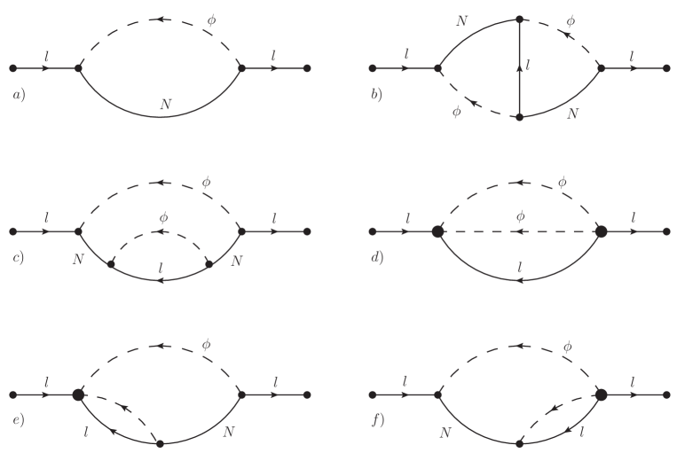
Refer to caption
Figure 3: One- and two-loop contributions to the lepton self-energy correspoding to washout terms, a) - d), and CP violating terms which generate a lepton asymmetry, e) and f).

To evaluate these graphs we need the correlation functions of lepton and Higgs fields in the thermal bath. A system in thermal equilibrium is described by the density matrix

ϱeq=exp(β(+μi𝒬i))Trexp(β(+μi𝒬i)),subscriptitalic-ϱ𝑒𝑞𝛽subscript𝜇𝑖subscript𝒬𝑖Tr𝛽subscript𝜇𝑖subscript𝒬𝑖\displaystyle\varrho_{eq}=\frac{\exp\left(\beta\left(-\mathcal{H}+\mu_{i}\mathcal{Q}_{i}\right)\right)}{{\rm Tr}\exp\left(\beta\left(-\mathcal{H}+\mu_{i}\mathcal{Q}_{i}\right)\right)}\ , (3.46)

where \mathcal{H} is the Hamiltonian of the system, β𝛽\beta is the inverse temperature, 𝒬isubscript𝒬𝑖\mathcal{Q}_{i} are conserved charges and μisubscript𝜇𝑖\mu_{i} are the corresponding chemical potentials. As expected for an initial state after inflation, we set all chemical potentials equal to zero.

Equilibrium correlation functions of a spatially homogeneous system only depend on space-time differences, and it is convenient to consider the Fourier transforms,

Δ𝐪±(ω)subscriptsuperscriptΔplus-or-minus𝐪𝜔\displaystyle\Delta^{\pm}_{\bf q}(\omega) =d4xei(ωx0𝐪𝐱)Δ±(x),absentsuperscript𝑑4𝑥superscript𝑒𝑖𝜔superscript𝑥0𝐪𝐱superscriptΔplus-or-minus𝑥\displaystyle=\int d^{4}xe^{i(\omega x^{0}-{\bf qx})}\Delta^{\pm}(x)\ , (3.47)
S𝐤±(ω)subscriptsuperscript𝑆plus-or-minus𝐤𝜔\displaystyle S^{\pm}_{\bf k}(\omega) =d4xei(ωx0𝐤𝐱)S±(x).absentsuperscript𝑑4𝑥superscript𝑒𝑖𝜔superscript𝑥0𝐤𝐱superscript𝑆plus-or-minus𝑥\displaystyle=\int d^{4}xe^{i(\omega x^{0}-{\bf kx})}S^{\pm}(x)\ . (3.48)

The equilibrium density matrix (3.46) then corresponds to a shift in imaginary time. This leads to the well-known Kubo-Martin-Schwinger (KMS) relations (cf. [44])

Δq<(ω)=eβωΔq>(ω),Sk<(ω)=eβωSk>(ω),formulae-sequencesubscriptsuperscriptΔq𝜔superscript𝑒𝛽𝜔subscriptsuperscriptΔq𝜔subscriptsuperscript𝑆k𝜔superscript𝑒𝛽𝜔subscriptsuperscript𝑆k𝜔\displaystyle\Delta^{<}_{\textbf{q}}(\omega)=e^{-\beta\omega}\Delta^{>}_{\textbf{q}}(\omega)\ ,\quad S^{<}_{\textbf{k}}(\omega)=-e^{-\beta\omega}S^{>}_{\textbf{k}}(\omega)\ , (3.49)

which imply

Δq+(ω)subscriptsuperscriptΔq𝜔\displaystyle\Delta^{+}_{\textbf{q}}(\omega) =i(12+fϕ(ω))Δq(ω)=i2coth(βω2)Δq(ω),absent𝑖12subscript𝑓italic-ϕ𝜔subscriptsuperscriptΔq𝜔𝑖2hyperbolic-cotangent𝛽𝜔2subscriptsuperscriptΔq𝜔\displaystyle=-i\left(\frac{1}{2}+f_{\phi}(\omega)\right)\Delta^{-}_{\textbf{q}}(\omega)=-\frac{i}{2}\coth\left(\frac{\beta\omega}{2}\right)\Delta^{-}_{\textbf{q}}(\omega)\ , (3.50)
Sk+(ω)subscriptsuperscript𝑆k𝜔\displaystyle S^{+}_{\textbf{k}}(\omega) =i(12fl(ω))Sk(ω)=i2tanh(βω2)Sk(ω),absent𝑖12subscript𝑓𝑙𝜔subscriptsuperscript𝑆k𝜔𝑖2𝛽𝜔2subscriptsuperscript𝑆k𝜔\displaystyle=-i\left(\frac{1}{2}-f_{l}(\omega)\right)S^{-}_{\textbf{k}}(\omega)=-\frac{i}{2}\tanh\left(\frac{\beta\omega}{2}\right)S^{-}_{\textbf{k}}(\omega)\ , (3.51)

where

fϕ(ω)=1eβω1,fl(ω)=1eβω+1,formulae-sequencesubscript𝑓italic-ϕ𝜔1superscript𝑒𝛽𝜔1subscript𝑓𝑙𝜔1superscript𝑒𝛽𝜔1\displaystyle f_{\phi}(\omega)=\frac{1}{e^{\beta\omega}-1}\ ,\quad f_{l}(\omega)=\frac{1}{e^{\beta\omega}+1}\ , (3.52)

are Bose-Einstein and Fermi-Dirac distribution functions, respectively. Note that the energy ω𝜔\omega is not on-shell.

Refer to caption
Figure 4: Path 𝒞βsubscript𝒞𝛽\mathcal{C}_{\beta} in the complex time plane for equilibrium correlation functions.

Equilibrium Green’s functions can be calculated in the real-time formalism using the contour 𝒞βsubscript𝒞𝛽\mathcal{C}_{\beta} in the complex time plane, which is shown in Fig. 4. For the free equilibrium propagators of massless lepton and Higgs fields one obtains (q=|𝐪|𝑞𝐪q=|{\bf q}|, k=|𝐤|𝑘𝐤k=|{\bf k}|, cf. [44]),

Δq(y)subscriptsuperscriptΔq𝑦\displaystyle\Delta^{-}_{\textbf{q}}(y) =1qsin(qy),absent1𝑞𝑞𝑦\displaystyle=\frac{1}{q}\sin(qy)\ , (3.53)
Δq+(y)subscriptsuperscriptΔq𝑦\displaystyle\Delta^{+}_{\textbf{q}}(y) =12qcoth(βq2)cos(qy),absent12𝑞hyperbolic-cotangent𝛽𝑞2𝑞𝑦\displaystyle=\frac{1}{2q}\coth\left(\frac{\beta q}{2}\right)\cos(qy)\ , (3.54)
SLk(y)subscriptsuperscript𝑆𝐿k𝑦\displaystyle S^{-}_{L\textbf{k}}(y) =PL(iγ0cos(ky)k𝜸ksin(ky)),absentsubscript𝑃𝐿𝑖subscript𝛾0𝑘𝑦k𝜸𝑘𝑘𝑦\displaystyle=P_{L}\left(i\gamma_{0}\cos(ky)-\frac{\textbf{k}\boldsymbol{\gamma}}{k}\sin(ky)\right)\ , (3.55)
SLk+(y)subscriptsuperscript𝑆𝐿k𝑦\displaystyle S^{+}_{L\textbf{k}}(y) =12PLtanh(βk2)(iγ0sin(ky)+k𝜸kcos(ky)).absent12subscript𝑃𝐿𝛽𝑘2𝑖subscript𝛾0𝑘𝑦k𝜸𝑘𝑘𝑦\displaystyle=-\frac{1}{2}P_{L}\tanh\left(\frac{\beta k}{2}\right)\left(i\gamma_{0}\sin(ky)+\frac{\textbf{k}\boldsymbol{\gamma}}{k}\cos(ky)\right)\ . (3.56)

All other propagators can be obtained as linear combinations using the relations described in the previous paragraph. A complete list is given in Appendix A.

In the following sections we shall see that the calculation of the lepton asymmetry represents an initial value problem which can be treated based on the real time formalism together with the Keldysh contour Fig. 2. Thermal and nonthermal properties of the system are then encoded in the initial values of the various Green’s functions.

4 Nonequilibrium correlation functions

The assumption of weak coupling to a large thermal bath with negligible backreaction in the framework of Kadanoff-Baym equations implies that self-energies for the heavy neutrinos N𝑁N are computed from equilibrium propagators of bath fields only. This also corresponds to a leading order perturbative expansion in the coupling constant.

Perturbative expansions of Boltzmann equations in multiscale problems are known to suffer from uncertainties, so-called secular terms, at late times. The Kadanoff-Baym equations (3.44) and (3.45) in full generality are free of secular terms and consistently include all memory effects. Nevertheless, the neglect of backreaction in the computation of ΣΣ\Sigma corresponds to a truncation in the perturbative expansion in the Yukawa couplings λ𝜆\lambda, which might introduce similar uncertainties related to the multiscale nature of the problem. However, in the system of consideration contributions of higher order in λ𝜆\lambda are not only suppressed by the smallness of the coupling, but also by the number of degrees of freedom in the bath that justify the neglect of backreaction. Hence, we expect potential problems due to secular terms not to be relevant.

The assumption that the background medium equilibrates instantaneously on the time scale of the asymmetry generation leaves open the details of the equilibration process. In reality, there are effects related to the finite equilibration time and the finite size of the quasi-particles. As we shall see in Section 5, these quantities play a crucial role in the Kadanoff-Baym result for the lepton asymmetry.

The self-energy for the heavy neutrino N𝑁N to leading order in λ𝜆\lambda is given by the diagram in Fig. 5.

\psfrag{p}{$\phi$}\psfrag{wp}{$(\omega_{\bf p},{\bf p})$}\psfrag{l}{$l$}\psfrag{N}{$N$}\includegraphics[width=216.81pt]{1loop}
Figure 5: One-loop contribution to the self-energies CΣ𝐩±𝐶subscriptsuperscriptΣplus-or-minus𝐩C\Sigma^{\pm}_{\bf p} of the Majorana neutrino N𝑁N.

It contains time-translation invariant propagators of bath fields only, and hence it is also time-translation invariant. As shown in [29], this implies that also the spectral function is time-translation invariant, G𝐩(t1,t2)G𝐩(y)subscriptsuperscript𝐺𝐩subscript𝑡1subscript𝑡2subscriptsuperscript𝐺𝐩𝑦G^{-}_{\bf p}(t_{1},t_{2})\equiv G^{-}_{\bf p}(y), y=t1t2𝑦subscript𝑡1subscript𝑡2y=t_{1}-t_{2}. In this case we can find the general solutions to the Kadanoff-Baym equations without further approximations.

4.1 Equation for the spectral function

Let us now consider the equation for the spectral function of the Majorana neutrino. After an obvious change of variables, the Kadanoff-Baym equation (3.44) becomes,

C(iγ0yp𝜸M)Gp(y)0y𝑑yCΣp(yy)Gp(y)=0.𝐶𝑖superscript𝛾0subscript𝑦p𝜸𝑀superscriptsubscript𝐺p𝑦superscriptsubscript0𝑦differential-dsuperscript𝑦𝐶superscriptsubscriptΣp𝑦superscript𝑦subscriptsuperscript𝐺psuperscript𝑦0\displaystyle C(i\gamma^{0}\partial_{y}-\textbf{p}\boldsymbol{\gamma}-M)G_{\textbf{p}}^{-}(y)-\int_{0}^{y}dy^{\prime}C\Sigma_{\textbf{p}}^{-}(y-y^{\prime})G^{-}_{\textbf{p}}(y^{\prime})=0\ . (4.1)

Defining the Laplace transform

G~p(s)=0𝑑yesyGp(y),Σ~p(s)=0𝑑yesyΣp(y),formulae-sequencesuperscriptsubscript~𝐺p𝑠superscriptsubscript0differential-d𝑦superscript𝑒𝑠𝑦subscriptsuperscript𝐺p𝑦superscriptsubscript~Σp𝑠superscriptsubscript0differential-d𝑦superscript𝑒𝑠𝑦subscriptsuperscriptΣp𝑦\displaystyle\tilde{G}_{\textbf{p}}^{-}(s)=\int_{0}^{\infty}dye^{-sy}G^{-}_{\textbf{p}}(y)\ ,\quad\tilde{\Sigma}_{\textbf{p}}^{-}(s)=\int_{0}^{\infty}dye^{-sy}\Sigma^{-}_{\textbf{p}}(y)\ , (4.2)

one obtains from Eq. (4.1)

(iγ0sp𝜸MΣ~p(s))G~p(s)=iγ0Gp(0).𝑖superscript𝛾0𝑠p𝜸𝑀subscriptsuperscript~Σp𝑠subscriptsuperscript~𝐺p𝑠𝑖superscript𝛾0subscriptsuperscript𝐺p0\displaystyle\left(i\gamma^{0}s-\textbf{p}\boldsymbol{\gamma}-M-\tilde{\Sigma}^{-}_{\textbf{p}}(s)\right)\tilde{G}^{-}_{\textbf{p}}(s)=i\gamma^{0}G^{-}_{\textbf{p}}(0)\ . (4.3)

Using the boundary condition (3.30),

Gp(0)=iγ0C1,subscriptsuperscript𝐺p0𝑖superscript𝛾0superscript𝐶1G^{-}_{\textbf{p}}(0)=i\gamma^{0}C^{-1}\ , (4.4)

this leads to

G~(s)=(iγ0sp𝜸MΣ~(s))1C1.superscript~𝐺𝑠superscript𝑖superscript𝛾0𝑠p𝜸𝑀superscript~Σ𝑠1superscript𝐶1\displaystyle\tilde{G}^{-}(s)=-\left(i\gamma^{0}s-\textbf{p}\boldsymbol{\gamma}-M-\tilde{\Sigma}^{-}(s)\right)^{-1}C^{-1}\ . (4.5)

The inverse Laplace transform is given by

Gp(y)=𝒞Bds2πiesyG~p(s),subscriptsuperscript𝐺p𝑦subscriptsubscript𝒞𝐵𝑑𝑠2𝜋𝑖superscript𝑒𝑠𝑦subscriptsuperscript~𝐺p𝑠\displaystyle G^{-}_{\textbf{p}}(y)=\int_{\mathcal{C}_{B}}\frac{ds}{2\pi i}e^{sy}\tilde{G}^{-}_{\textbf{p}}(s)\ , (4.6)

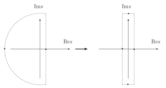
where 𝒞Bsubscript𝒞𝐵\mathcal{C}_{B} is the Bromwich contour (see Fig. 6): The part parallel to the imaginary axis is chosen such that all singularities of the integrand are to its left; the second part is the semicircle at infinity which closes the contour at Re(s)<0Re𝑠0{\rm Re}(s)<0.

Refer to caption
Figure 6: Bromwich contour

From the definition of the Laplace transform one can see that the self-energy Σ~p(s)subscriptsuperscript~Σp𝑠\tilde{\Sigma}^{-}_{\textbf{p}}(s) is analytic on the real s𝑠s axis, but has a discontinuity across the imaginary axis. This gives rise to the spectral representation

Σ~p(s)=idp02πΣp(p0)isp0.subscriptsuperscript~Σp𝑠𝑖superscriptsubscript𝑑subscript𝑝02𝜋subscriptsuperscriptΣpsubscript𝑝0𝑖𝑠subscript𝑝0\displaystyle\tilde{\Sigma}^{-}_{\textbf{p}}(s)=i\int_{-\infty}^{\infty}\frac{dp_{0}}{2\pi}\frac{\Sigma^{-}_{\textbf{p}}(p_{0})}{is-p_{0}}\ . (4.7)

Note that the retarded and advanced self-energies are given by

Σ~p(iω+ϵ)subscriptsuperscript~Σp𝑖𝜔italic-ϵ\displaystyle\tilde{\Sigma}^{-}_{\textbf{p}}(-i\omega+\epsilon) =ΣpR(ω),absentsubscriptsuperscriptΣ𝑅p𝜔\displaystyle=\Sigma^{R}_{\textbf{p}}(\omega)\ , (4.8)
Σ~p(iωϵ)subscriptsuperscript~Σp𝑖𝜔italic-ϵ\displaystyle\tilde{\Sigma}^{-}_{\textbf{p}}(-i\omega-\epsilon) =ΣpA(ω).absentsubscriptsuperscriptΣ𝐴p𝜔\displaystyle=\Sigma^{A}_{\textbf{p}}(\omega)\ . (4.9)

These self-energies are determined by the discontinuity of Σ~p(s)subscriptsuperscript~Σp𝑠\tilde{\Sigma}^{-}_{\textbf{p}}(s),

discΣ~p(iω)=Σ~p(iω+ϵ)Σ~p(iωϵ)=Σp(ω),discsubscriptsuperscript~Σp𝑖𝜔subscriptsuperscript~Σp𝑖𝜔italic-ϵsubscriptsuperscript~Σp𝑖𝜔italic-ϵsubscriptsuperscriptΣp𝜔\displaystyle\mathrm{disc}\tilde{\Sigma}^{-}_{\textbf{p}}(-i\omega)=\tilde{\Sigma}^{-}_{\textbf{p}}(-i\omega+\epsilon)-\tilde{\Sigma}^{-}_{\textbf{p}}(-i\omega-\epsilon)=\Sigma^{-}_{\textbf{p}}(\omega)\ , (4.10)

with the real part given by the principal value, i.e.,

Σ~p(iω±ϵ)=i𝒫dp02πΣ(p0)ωp0±12Σp(ω).subscriptsuperscript~Σpplus-or-minus𝑖𝜔italic-ϵplus-or-minus𝑖𝒫superscriptsubscript𝑑subscript𝑝02𝜋superscriptΣsubscript𝑝0𝜔subscript𝑝012subscriptsuperscriptΣp𝜔\displaystyle\tilde{\Sigma}^{-}_{\textbf{p}}(-i\omega\pm\epsilon)=i\mathcal{P}\int_{-\infty}^{\infty}\frac{dp_{0}}{2\pi}\frac{\Sigma^{-}(p_{0})}{\omega-p_{0}}\pm\frac{1}{2}\Sigma^{-}_{\textbf{p}}(\omega)\ . (4.11)

This representation of the self-energy is familiar from the theory at zero temperature.

We are now ready to calculate the spectral function in terms of the self-energy Σp(ω)subscriptsuperscriptΣp𝜔\Sigma^{-}_{\textbf{p}}(\omega). Its Laplace transform has singularities only on the imaginary axis. Hence the Bromwich contour can be deformed as 𝒞Bi+ϵi+ϵ+iϵiϵsubscript𝒞𝐵subscriptsuperscript𝑖italic-ϵ𝑖italic-ϵsubscriptsuperscript𝑖italic-ϵ𝑖italic-ϵ\mathcal{C}_{B}\to\int^{i\infty+\epsilon}_{-i\infty+\epsilon}+\int^{-i\infty-\epsilon}_{i\infty-\epsilon} (see Fig. 6), which yields for the spectral function

Gp(y)subscriptsuperscript𝐺p𝑦\displaystyle G^{-}_{\textbf{p}}(y) =𝒞Bds2πiesyG~p(s)absentsubscriptsubscript𝒞𝐵𝑑𝑠2𝜋𝑖superscript𝑒𝑠𝑦subscriptsuperscript~𝐺p𝑠\displaystyle=\int_{\mathcal{C}_{B}}\frac{ds}{2\pi i}e^{sy}\tilde{G}^{-}_{\textbf{p}}(s)
=dω2πe(iω+ϵ)yG~p(iω+ϵ)+dω2πe(iωϵ)yG~p(iωϵ)absentsuperscriptsubscript𝑑𝜔2𝜋superscript𝑒𝑖𝜔italic-ϵ𝑦subscriptsuperscript~𝐺p𝑖𝜔italic-ϵsuperscriptsubscript𝑑𝜔2𝜋superscript𝑒𝑖𝜔italic-ϵ𝑦subscriptsuperscript~𝐺p𝑖𝜔italic-ϵ\displaystyle=\int_{-\infty}^{\infty}\frac{d\omega}{2\pi}e^{(i\omega+\epsilon)y}\tilde{G}^{-}_{\textbf{p}}(i\omega+\epsilon)+\int_{\infty}^{-\infty}\frac{d\omega}{2\pi}e^{(i\omega-\epsilon)y}\tilde{G}^{-}_{\textbf{p}}(i\omega-\epsilon)
=dω2πeiωy(G~p(iω+ϵ)G~p(iωϵ)).absentsuperscriptsubscript𝑑𝜔2𝜋superscript𝑒𝑖𝜔𝑦subscriptsuperscript~𝐺p𝑖𝜔italic-ϵsubscriptsuperscript~𝐺p𝑖𝜔italic-ϵ\displaystyle=\int_{-\infty}^{\infty}\frac{d\omega}{2\pi}e^{-i\omega y}\left(\tilde{G}^{-}_{\textbf{p}}(-i\omega+\epsilon)-\tilde{G}^{-}_{\textbf{p}}(-i\omega-\epsilon)\right)\ . (4.12)

The Fourier transform of the spectral function,

ρp(ω)=i𝑑yeiωyGp(y),subscript𝜌p𝜔𝑖superscriptsubscriptdifferential-d𝑦superscript𝑒𝑖𝜔𝑦subscriptsuperscript𝐺p𝑦\displaystyle\rho_{\textbf{p}}(\omega)=-i\int_{-\infty}^{\infty}dye^{i\omega y}G^{-}_{\textbf{p}}(y)\ , (4.13)

is then given by

ρp(ω)=(iM12Σp(ω)iM+12Σp(ω))C1.subscript𝜌p𝜔𝑖italic-p̸𝑀12subscriptsuperscriptΣp𝜔𝑖italic-p̸𝑀12subscriptsuperscriptΣp𝜔superscript𝐶1\displaystyle\rho_{\textbf{p}}(\omega)=\left(\frac{-i}{\displaystyle{\not}{p}-M-\frac{1}{2}\Sigma^{-}_{\textbf{p}}(\omega)}-\frac{-i}{\displaystyle{\not}{p}-M+\frac{1}{2}\Sigma^{-}_{\textbf{p}}(\omega)}\right)C^{-1}\ . (4.14)

Here we have assumed that the divergent contribution of the real part has already been absorbed into mass and wave function renormalization, so that ρp(ω)subscript𝜌p𝜔\rho_{\textbf{p}}(\omega) represents the renormalized spectral density. The finite part of the self-energy is negligable because of the small Yukawa coupling.

A straightforward calculation yields for the self-energy (cf. [35]),

Σp(ω)=2i(λλ)11𝐤,𝐪σ(p;k,q),subscriptsuperscriptΣp𝜔2𝑖subscriptsuperscript𝜆𝜆11subscript𝐤𝐪italic-k̸𝜎𝑝𝑘𝑞\displaystyle\Sigma^{-}_{\textbf{p}}(\omega)=2i\left(\lambda^{\dagger}\lambda\right)_{11}\int_{\bf k,q}\displaystyle{\not}{k}\ \sigma(p;k,q)\ , (4.15)

where we have defined

σ(p;k,q)=𝜎𝑝𝑘𝑞absent\displaystyle\sigma(p;k,q)= flϕ(k,q)(2π)4(δ4(pkq)+δ4(p+k+q))subscript𝑓𝑙italic-ϕ𝑘𝑞superscript2𝜋4superscript𝛿4𝑝𝑘𝑞superscript𝛿4𝑝𝑘𝑞\displaystyle\;f_{l\phi}(k,q)(2\pi)^{4}\left(\delta^{4}(p-k-q)+\delta^{4}(p+k+q)\right)
+f¯lϕ(k,q)(2π)4(δ4(p+kq)+δ4(pk+q)),subscript¯𝑓𝑙italic-ϕ𝑘𝑞superscript2𝜋4superscript𝛿4𝑝𝑘𝑞superscript𝛿4𝑝𝑘𝑞\displaystyle+\bar{f}_{l\phi}(k,q)(2\pi)^{4}\left(\delta^{4}(p+k-q)+\delta^{4}(p-k+q)\right)\ , (4.16)

with the statistical factors

flϕ(k,q)=1fl(k)+fϕ(q),f¯lϕ(k,q)=fϕ(q)+fl(k).formulae-sequencesubscript𝑓𝑙italic-ϕ𝑘𝑞1subscript𝑓𝑙𝑘subscript𝑓italic-ϕ𝑞subscript¯𝑓𝑙italic-ϕ𝑘𝑞subscript𝑓italic-ϕ𝑞subscript𝑓𝑙𝑘\displaystyle f_{l\phi}(k,q)=1-f_{l}(k)+f_{\phi}(q)\ ,\quad\bar{f}_{l\phi}(k,q)=f_{\phi}(q)+f_{l}(k)\ . (4.17)

Note that k𝑘k and q𝑞q are on-shell, i.e., k=(k,𝐤)𝑘𝑘𝐤k=(k,{\bf k}) and q=(q,𝐪)𝑞𝑞𝐪q=(q,{\bf q}), whereas p=(ω,𝐩)𝑝𝜔𝐩p=(\omega,{\bf p}) is off-shell. The properties of the Dirac matrices and rotational invariance imply

Σp(ω)=iap(ω)γ0+ibp(ω)p𝜸,subscriptsuperscriptΣp𝜔𝑖subscript𝑎p𝜔superscript𝛾0𝑖subscript𝑏p𝜔p𝜸\displaystyle\Sigma^{-}_{\textbf{p}}(\omega)=ia_{\textbf{p}}(\omega)\gamma^{0}+ib_{\textbf{p}}(\omega)\textbf{p}\boldsymbol{\gamma}\ , (4.18)

where

ap(ω)subscript𝑎p𝜔\displaystyle a_{\textbf{p}}(\omega) =2(λλ)11𝐪,𝐤kσ(p;k,q),absent2subscriptsuperscript𝜆𝜆11subscript𝐪𝐤𝑘𝜎𝑝𝑘𝑞\displaystyle=2\left(\lambda^{\dagger}\lambda\right)_{11}\int_{\bf q,k}{k}\ \sigma(p;k,q)\ , (4.19)
bp(ω)subscript𝑏p𝜔\displaystyle b_{\textbf{p}}(\omega) =2(λλ)111p2𝐪,𝐤pkσ(p;k,q).absent2subscriptsuperscript𝜆𝜆111superscriptp2subscript𝐪𝐤pk𝜎𝑝𝑘𝑞\displaystyle=-2\left(\lambda^{\dagger}\lambda\right)_{11}\frac{1}{\textbf{p}^{2}}\int_{\bf q,k}\textbf{p}\textbf{k}\ \sigma(p;k,q)\ . (4.20)

These functions satisfy the relations

ap(ωp)=ap(ωp),bp(ωp)=bp(ωp).formulae-sequencesubscript𝑎psubscript𝜔psubscript𝑎psubscript𝜔psubscript𝑏psubscript𝜔psubscript𝑏psubscript𝜔p\displaystyle a_{\textbf{p}}(-\omega_{\textbf{p}})=a_{\textbf{p}}(\omega_{\textbf{p}})\ ,\quad b_{\textbf{p}}(-\omega_{\textbf{p}})=-b_{\textbf{p}}(\omega_{\textbf{p}})\ . (4.21)

Using Eq. (4.18) and linearising the denominators in Eq. (4.14) in the small quantities ap(ω)subscript𝑎p𝜔a_{\textbf{p}}(\omega) and bp(ω)subscript𝑏p𝜔b_{\textbf{p}}(\omega), one obtains for the spectral density

ρp(ω)=2ωΓp(ω)(ω2ωp2)+(ωΓp(ω))2(+M)C1,subscript𝜌p𝜔2𝜔subscriptΓp𝜔superscript𝜔2superscriptsubscript𝜔p2superscript𝜔subscriptΓp𝜔2italic-p̸𝑀superscript𝐶1\displaystyle\rho_{\textbf{p}}(\omega)=\frac{2\omega\Gamma_{\textbf{p}}(\omega)}{\left(\omega^{2}-\omega_{\textbf{p}}^{2}\right)+\left(\omega\Gamma_{\textbf{p}}(\omega)\right)^{2}}\left(\displaystyle{\not}{p}+M\right)C^{-1}\ , (4.22)

where

ωΓp(ω)𝜔subscriptΓp𝜔\displaystyle\omega\Gamma_{\textbf{p}}(\omega) =ωap(ω)+p2bp(ω)absent𝜔subscript𝑎p𝜔superscriptp2subscript𝑏p𝜔\displaystyle=\omega a_{\textbf{p}}(\omega)+\textbf{p}^{2}b_{\textbf{p}}(\omega)
=2(λλ)11𝐪,𝐤pkσ(p;k,q).absent2subscriptsuperscript𝜆𝜆11subscript𝐪𝐤𝑝𝑘𝜎𝑝𝑘𝑞\displaystyle=2\left(\lambda^{\dagger}\lambda\right)_{11}\int_{\bf q,k}\ p\cdot k\ \sigma(p;k,q)\ . (4.23)

On-shell, only the first of the δ𝛿\delta-functions in σ(p;k,q)𝜎𝑝𝑘𝑞\sigma(p;k,q) contributes, and one obtains the width appearing in the Boltzmann equations,

Γp(ωp)=(λλ)112ωp𝐪,𝐤pkflϕ(k,q)(2π)4δ4(pkq)Γp,subscriptΓpsubscript𝜔psubscriptsuperscript𝜆𝜆112subscript𝜔psubscript𝐪𝐤𝑝𝑘subscript𝑓𝑙italic-ϕ𝑘𝑞superscript2𝜋4superscript𝛿4𝑝𝑘𝑞subscriptΓp\displaystyle\Gamma_{\textbf{p}}(\omega_{\textbf{p}})=\left(\lambda^{\dagger}\lambda\right)_{11}\frac{2}{\omega_{\textbf{p}}}\int_{\bf q,k}\ p\cdot k\ f_{l\phi}(k,q)(2\pi)^{4}\delta^{4}(p-k-q)\equiv\Gamma_{\textbf{p}}\ , (4.24)

which satisfies the relations

Γp(ωp)=Γp(ωp)=Γp(ωp).subscriptΓpsubscript𝜔psubscriptΓpsubscript𝜔psubscriptΓpsubscript𝜔p\displaystyle\Gamma_{\textbf{p}}(-\omega_{\textbf{p}})=\Gamma_{-\textbf{p}}(\omega_{\textbf{p}})=\Gamma_{\textbf{p}}(\omega_{\textbf{p}})\ . (4.25)

In the zero-width limit the spectral function (4.22) reduces to the familiar expression in vacuum,

ρp(ω)=2πsign(ω)δ(p2M2)(+M)C1.subscript𝜌p𝜔2𝜋sign𝜔𝛿superscript𝑝2superscript𝑀2italic-p̸𝑀superscript𝐶1\rho_{\textbf{p}}(\omega)=2\pi{\rm sign}(\omega)\delta(p^{2}-M^{2})(\displaystyle{\not}{p}+M)C^{-1}\ . (4.26)

The spectral propagator is now obtained by evaluating the Fourier transform of the spectral function (4.22),

G𝐩(y)=idω2πeiωyρ𝐩(ω),superscriptsubscript𝐺𝐩𝑦𝑖subscriptsuperscript𝑑𝜔2𝜋superscript𝑒𝑖𝜔𝑦subscript𝜌𝐩𝜔\displaystyle G_{\bf p}^{-}(y)=i\int^{\infty}_{-\infty}\frac{d\omega}{2\pi}e^{-i\omega y}\rho_{{\bf p}}(\omega)\ , (4.27)

which yields the final result

G𝐩(y)=(iγ0cos(ω𝐩y)+Mp𝜸ω𝐩sin(ω𝐩y))eΓ𝐩|y|/2C1.superscriptsubscript𝐺𝐩𝑦𝑖subscript𝛾0subscript𝜔𝐩𝑦𝑀p𝜸subscript𝜔𝐩subscript𝜔𝐩𝑦superscript𝑒subscriptΓ𝐩𝑦2superscript𝐶1\displaystyle G_{\bf p}^{-}(y)=\left(i\gamma_{0}\cos(\omega_{\bf p}y)+\frac{M-\textbf{p}\boldsymbol{\gamma}}{\omega_{\bf p}}\sin(\omega_{\bf p}y)\right)e^{-\Gamma_{\bf p}|y|/2}C^{-1}\ . (4.28)

Compared to the free spectral function only an exponential damping factor appears. This is a feature of the narrow-width approximation, analogous to the scalar field case discussed in [29].

4.2 Equation for the statistical propagator

We now proceed to the solution of the second Kadanoff-Baym equation (3.45) which, choosing ti=0subscript𝑡𝑖0t_{i}=0, reads

C(iγ0t1p𝜸M)G𝐩+(t1,t2)0t1𝑑tCΣ𝐩(t1t)G𝐩+(t,t2)=ζ𝐩(t1t2),𝐶𝑖superscript𝛾0subscriptsubscript𝑡1p𝜸𝑀superscriptsubscript𝐺𝐩subscript𝑡1subscript𝑡2subscriptsuperscriptsubscript𝑡10differential-dsuperscript𝑡𝐶subscriptsuperscriptΣ𝐩subscript𝑡1superscript𝑡superscriptsubscript𝐺𝐩superscript𝑡subscript𝑡2subscript𝜁𝐩subscript𝑡1subscript𝑡2\displaystyle C(i\gamma^{0}\partial_{t_{1}}-\textbf{p}\boldsymbol{\gamma}-M)G_{\bf p}^{+}(t_{1},t_{2})-\int^{t_{1}}_{0}dt^{\prime}C\Sigma^{-}_{\bf p}(t_{1}-t^{\prime})G_{\bf p}^{+}(t^{\prime},t_{2})=\zeta_{\bf p}(t_{1}-t_{2})\ , (4.29)

with the source term

ζ𝐩(t1t2)=0t2𝑑tΣ𝐩+(t1t)G𝐩(tt2).subscript𝜁𝐩subscript𝑡1subscript𝑡2subscriptsuperscriptsubscript𝑡20differential-dsuperscript𝑡superscriptsubscriptΣ𝐩subscript𝑡1superscript𝑡superscriptsubscript𝐺𝐩superscript𝑡subscript𝑡2\displaystyle\zeta_{\bf p}(t_{1}-t_{2})=-\int^{t_{2}}_{0}dt^{\prime}\Sigma_{\bf p}^{+}(t_{1}-t^{\prime})G_{\bf p}^{-}(t^{\prime}-t_{2})\ . (4.30)

The general solution of (4.29) takes the form

G𝐩+(t1,t2)=G^𝐩+(t1,t2)+G𝐩,mem+(t1,t2),superscriptsubscript𝐺𝐩subscript𝑡1subscript𝑡2superscriptsubscript^𝐺𝐩subscript𝑡1subscript𝑡2superscriptsubscript𝐺𝐩memsubscript𝑡1subscript𝑡2\displaystyle G_{\bf p}^{+}(t_{1},t_{2})=\hat{G}_{\bf p}^{+}(t_{1},t_{2})+G_{{\bf p},{\rm mem}}^{+}(t_{1},t_{2})\ , (4.31)

where G^𝐩+(t1,t2)superscriptsubscript^𝐺𝐩subscript𝑡1subscript𝑡2\hat{G}_{\bf p}^{+}(t_{1},t_{2}) is the general solution of the homogeneous equation

C(iγ0t1p𝜸M)G^𝐩+(t1,t2)0t1𝑑tCΣ𝐩(t1t)G^𝐩+(t,t2)=0,𝐶𝑖superscript𝛾0subscriptsubscript𝑡1p𝜸𝑀superscriptsubscript^𝐺𝐩subscript𝑡1subscript𝑡2subscriptsuperscriptsubscript𝑡10differential-dsuperscript𝑡𝐶subscriptsuperscriptΣ𝐩subscript𝑡1superscript𝑡superscriptsubscript^𝐺𝐩superscript𝑡subscript𝑡20\displaystyle C(i\gamma^{0}\partial_{t_{1}}-\textbf{p}\boldsymbol{\gamma}-M)\hat{G}_{{\bf p}}^{+}(t_{1},t_{2})-\int^{t_{1}}_{0}dt^{\prime}C\Sigma^{-}_{\bf p}(t_{1}-t^{\prime})\hat{G}_{\bf p}^{+}(t^{\prime},t_{2})=0\ , (4.32)

and the ‘memory integral’, which contains non-Markovian effects, is given by

G𝐩,mem+(t1,t2)=0t1𝑑t0t2𝑑t′′G𝐩(t1t)Σ𝐩+(tt′′)G𝐩(t′′t2).subscriptsuperscript𝐺𝐩memsubscript𝑡1subscript𝑡2subscriptsuperscriptsubscript𝑡10differential-dsuperscript𝑡subscriptsuperscriptsubscript𝑡20differential-dsuperscript𝑡′′superscriptsubscript𝐺𝐩subscript𝑡1superscript𝑡superscriptsubscriptΣ𝐩superscript𝑡superscript𝑡′′superscriptsubscript𝐺𝐩superscript𝑡′′subscript𝑡2G^{+}_{{\bf p},{\rm mem}}(t_{1},t_{2})=\int^{t_{1}}_{0}dt^{\prime}\int^{t_{2}}_{0}dt^{\prime\prime}G_{\bf p}^{-}(t_{1}-t^{\prime})\Sigma_{\bf p}^{+}(t^{\prime}-t^{\prime\prime})G_{\bf p}^{-}(t^{\prime\prime}-t_{2})\ . (4.33)

One easily verifies that the memory integral is a special solution of the inhomogeneous equation.

In order to evaluate the memory integral we perform a Fourier transform of the self-energy (y=t1t2𝑦subscript𝑡1subscript𝑡2y=t_{1}-t_{2}),

G𝐩,mem+superscriptsubscript𝐺𝐩mem\displaystyle G_{{\bf p},{\rm mem}}^{+} (t1,t2)=subscript𝑡1subscript𝑡2absent\displaystyle(t_{1},t_{2})=
dω2π(0t1𝑑y1G𝐩(y1)eiωy1)Σ𝐩+(ω)(0t2𝑑y2G𝐩(y2)eiωy2)eiωy.𝑑𝜔2𝜋superscriptsubscript0subscript𝑡1differential-dsubscript𝑦1superscriptsubscript𝐺𝐩subscript𝑦1superscript𝑒𝑖𝜔subscript𝑦1superscriptsubscriptΣ𝐩𝜔superscriptsubscript0subscript𝑡2differential-dsubscript𝑦2superscriptsubscript𝐺𝐩subscript𝑦2superscript𝑒𝑖𝜔subscript𝑦2superscript𝑒𝑖𝜔𝑦\displaystyle\int\frac{d\omega}{2\pi}\left(\int_{0}^{t_{1}}dy_{1}G_{\bf p}^{-}(y_{1})e^{i\omega y_{1}}\right)\Sigma_{\bf p}^{+}(\omega)\left(\int_{0}^{t_{2}}dy_{2}G_{\bf p}^{-}(-y_{2})e^{-i\omega y_{2}}\right)e^{-i\omega y}\ . (4.34)

Since the self-energy is computed with fields in thermal equilibrium, it satisfies the KMS condition (cf. (3.51))

Σ𝐩+(ω)=i2tanh(βω2)Σ𝐩(ω).superscriptsubscriptΣ𝐩𝜔𝑖2𝛽𝜔2superscriptsubscriptΣ𝐩𝜔\Sigma_{\bf p}^{+}(\omega)=-\frac{i}{2}\tanh\left(\frac{\beta\omega}{2}\right)\Sigma_{\bf p}^{-}(\omega)\ . (4.35)

Using the expressions (4.18) and (4.28) for self-energy and spectral function, respectively, which were derived in the previous section, it is now straightforward to calculate the memory integral explicitly. Neglecting terms 𝒪(Γp)𝒪subscriptΓp\mathcal{O}(\Gamma_{\textbf{p}}) in the numerator, one finds

0t𝑑yeiωyG𝐩(y)superscriptsubscript0𝑡differential-d𝑦superscript𝑒𝑖𝜔𝑦superscriptsubscript𝐺𝐩𝑦\displaystyle\int_{0}^{t}dye^{i\omega y}G_{\bf p}^{-}(y)\ =1ωp2(ω+iΓ𝐩/2)2×\displaystyle=\frac{1}{\omega_{\textbf{p}}^{2}-(\omega+i\Gamma_{\bf p}/2)^{2}}\ \times (4.36)
(iγ0[(ωpsin(ωpt)+iωcos(ωpt))ei(ω+iΓ𝐩/2)tiω]\displaystyle\Big{(}i\gamma^{0}\big{[}\big{(}\omega_{\textbf{p}}\sin(\omega_{\textbf{p}}t)+i\omega\cos(\omega_{\textbf{p}}t)\big{)}e^{i(\omega+i\Gamma_{\bf p}/2)t}-i\omega\big{]}
+M𝐩𝜸ωp[iω(sin(ωpt)ωpcos(ωpt))ei(ω+iΓ𝐩/2)t+ωp])C1,\displaystyle+\frac{M-{\bf p}\boldsymbol{\gamma}}{\omega_{\textbf{p}}}\big{[}i\omega\big{(}\sin(\omega_{\textbf{p}}t)-\omega_{\textbf{p}}\cos(\omega_{\textbf{p}}t)\big{)}e^{i(\omega+i\Gamma_{\bf p}/2)t}+\omega_{\textbf{p}}\big{]}\Big{)}C^{-1}\ ,
0t𝑑yeiωyG𝐩(y)superscriptsubscript0𝑡differential-d𝑦superscript𝑒𝑖𝜔𝑦superscriptsubscript𝐺𝐩𝑦\displaystyle\int_{0}^{t}dye^{-i\omega y}G_{\bf p}^{-}(-y)\ =1ωp2(ωiΓ𝐩/2)2×\displaystyle=\frac{1}{\omega_{\textbf{p}}^{2}-(\omega-i\Gamma_{\bf p}/2)^{2}}\ \times (4.37)
(iγ0[(ωpsin(ωpt)iωcos(ωpt))ei(ωiΓ𝐩/2)tiω]\displaystyle\Big{(}i\gamma^{0}\big{[}\big{(}\omega_{\textbf{p}}\sin(\omega_{\textbf{p}}t)-i\omega\cos(\omega_{\textbf{p}}t)\big{)}e^{-i(\omega-i\Gamma_{\bf p}/2)t}-i\omega\big{]}
+M𝐩𝜸ωp[iω(sin(ωpt)ωpcos(ωpt))ei(ω+iΓ𝐩/2)t+ωp])C1.\displaystyle+\frac{M-{\bf p}\boldsymbol{\gamma}}{\omega_{\textbf{p}}}\big{[}i\omega\big{(}\sin(\omega_{\textbf{p}}t)-\omega_{\textbf{p}}\cos(\omega_{\textbf{p}}t)\big{)}e^{i(\omega+i\Gamma_{\bf p}/2)t}+\omega_{\textbf{p}}\big{]}\Big{)}C^{-1}\ .

After inserting these expressions in Eq. (4.2) one can perform the ω𝜔\omega-integration using Cauchy’s theorem. The integrand has two poles777There are further poles at ωn=±iπ(1+2n)/βsubscript𝜔𝑛plus-or-minus𝑖𝜋12𝑛𝛽\omega_{n}=\pm i\pi(1+2n)/\beta, n𝑛n integer. However, their contribution to G𝐩,mem+superscriptsubscript𝐺𝐩memG_{{\bf p},{\rm mem}}^{+} is 𝒪(Γ𝐩/M)𝒪subscriptΓ𝐩𝑀{\cal O}(\Gamma_{\bf p}/M) and therefore negligible. in the upper-half plane at ω=iΓ𝐩/2±ωp𝜔plus-or-minus𝑖subscriptΓ𝐩2subscript𝜔p\omega=i\Gamma_{\bf p}/2\pm\omega_{\textbf{p}}, and two poles in the lower-half plane ω=iΓ𝐩/2±ωp𝜔plus-or-minus𝑖subscriptΓ𝐩2subscript𝜔p\omega=-i\Gamma_{\bf p}/2\pm\omega_{\textbf{p}}. The choice of the contour depends on the sign of the time variables in the exponent. The result is a sum of the contributions from all four poles. The expressions appearing in the numerator can be simplified by means of Eqs. (4.21) and (4.24) for self-energy and equilibration width, respectively,

(γ0+M𝐩𝜸ωp)Σp(ωp)(γ0+M𝐩𝜸ωp)superscript𝛾0𝑀𝐩𝜸subscript𝜔psubscriptsuperscriptΣpsubscript𝜔psuperscript𝛾0𝑀𝐩𝜸subscript𝜔p\displaystyle\Big{(}\gamma^{0}+\frac{M-{\bf p}\boldsymbol{\gamma}}{\omega_{\textbf{p}}}\Big{)}\Sigma^{-}_{\textbf{p}}(\omega_{\textbf{p}})\Big{(}\gamma^{0}+\frac{M-{\bf p}\boldsymbol{\gamma}}{\omega_{\textbf{p}}}\Big{)} =2iΓ𝐩(γ0+M𝐩𝜸ωp),absent2𝑖subscriptΓ𝐩superscript𝛾0𝑀𝐩𝜸subscript𝜔p\displaystyle=2i\Gamma_{\bf p}\Big{(}\gamma^{0}+\frac{M-{\bf p}\boldsymbol{\gamma}}{\omega_{\textbf{p}}}\Big{)}\ , (4.38)
(γ0M𝐩𝜸ωp)Σp(ωp)(γ0M𝐩𝜸ωp)superscript𝛾0𝑀𝐩𝜸subscript𝜔psubscriptsuperscriptΣpsubscript𝜔psuperscript𝛾0𝑀𝐩𝜸subscript𝜔p\displaystyle\Big{(}\gamma^{0}-\frac{M-{\bf p}\boldsymbol{\gamma}}{\omega_{\textbf{p}}}\Big{)}\Sigma^{-}_{\textbf{p}}(-\omega_{\textbf{p}})\Big{(}\gamma^{0}-\frac{M-{\bf p}\boldsymbol{\gamma}}{\omega_{\textbf{p}}}\Big{)} =2iΓ𝐩(γ0M𝐩𝜸ωp).absent2𝑖subscriptΓ𝐩superscript𝛾0𝑀𝐩𝜸subscript𝜔p\displaystyle=2i\Gamma_{\bf p}\Big{(}\gamma^{0}-\frac{M-{\bf p}\boldsymbol{\gamma}}{\omega_{\textbf{p}}}\Big{)}\ . (4.39)

Using these expressions one finally obtains for the memory integral, changing variables from (t1,t2)subscript𝑡1subscript𝑡2(t_{1},t_{2}) to (t,y)𝑡𝑦(t,y),

Gp,mem+(t,y)=subscriptsuperscript𝐺pmem𝑡𝑦absent\displaystyle G^{+}_{\textbf{p},{\rm mem}}(t,y)= (4.40)
12tanh(βωp2)(iγ0sin(ωpy)Mp𝜸ωpcos(ωpy))(eΓ𝐪|y|/2eΓ𝐪t)C1.12𝛽subscript𝜔p2𝑖subscript𝛾0subscript𝜔p𝑦𝑀p𝜸subscript𝜔psubscript𝜔p𝑦superscript𝑒subscriptΓ𝐪𝑦2superscript𝑒subscriptΓ𝐪𝑡superscript𝐶1\displaystyle\;-\frac{1}{2}\tanh\left(\frac{\beta\omega_{\textbf{p}}}{2}\right)\left(i\gamma_{0}\sin(\omega_{\textbf{p}}y)-\frac{M-\textbf{p}\boldsymbol{\gamma}}{\omega_{\textbf{p}}}\cos(\omega_{\textbf{p}}y)\right)\left(e^{-\Gamma_{{\bf q}}|y|/2}-e^{-\Gamma_{{\bf q}}t}\right)C^{-1}\ .

Asymptotically, for t𝑡t\rightarrow\infty, the memory integral becomes

Gp+eq(t,y)=12tanh(βωp2)(iγ0sin(ωpy)Mp𝜸ωpcos(ωpy))eΓ𝐪|y|/2C1.subscriptsuperscript𝐺eqp𝑡𝑦12𝛽subscript𝜔p2𝑖subscript𝛾0subscript𝜔p𝑦𝑀p𝜸subscript𝜔psubscript𝜔p𝑦superscript𝑒subscriptΓ𝐪𝑦2superscript𝐶1\displaystyle G^{+\mathrm{eq}}_{\textbf{p}}(t,y)=-\frac{1}{2}\tanh\left(\frac{\beta\omega_{\textbf{p}}}{2}\right)\left(i\gamma_{0}\sin(\omega_{\textbf{p}}y)-\frac{M-\textbf{p}\boldsymbol{\gamma}}{\omega_{\textbf{p}}}\cos(\omega_{\textbf{p}}y)\right)e^{-\Gamma_{{\bf q}}|y|/2}C^{-1}\ . (4.41)

One easily verifies that Gp+eq(t,y)subscriptsuperscript𝐺eqp𝑡𝑦G^{+\mathrm{eq}}_{\textbf{p}}(t,y) indeed represents the equilibrium statistical propagator. For the Fourier transform one obtains

Gp+eq(ω)subscriptsuperscript𝐺eqp𝜔\displaystyle G^{+\mathrm{eq}}_{\textbf{p}}(\omega) =𝑑yeiωyGp+eq(y)absentsuperscriptsubscriptdifferential-d𝑦superscript𝑒𝑖𝜔𝑦subscriptsuperscript𝐺eqp𝑦\displaystyle=\int_{-\infty}^{\infty}dye^{i\omega y}G^{+\mathrm{eq}}_{\textbf{p}}(y)
=12tanh(βω2)2ωΓp(ω)(ω2ωp2)+(ωΓp(ω))2(+M)C1absent12𝛽𝜔22𝜔subscriptΓp𝜔superscript𝜔2superscriptsubscript𝜔p2superscript𝜔subscriptΓp𝜔2italic-p̸𝑀superscript𝐶1\displaystyle=\frac{1}{2}\tanh\left(\frac{\beta\omega}{2}\right)\frac{2\omega\Gamma_{\textbf{p}}(\omega)}{\left(\omega^{2}-\omega_{\textbf{p}}^{2}\right)+\left(\omega\Gamma_{\textbf{p}}(\omega)\right)^{2}}\left(\displaystyle{\not}{p}+M\right)C^{-1}
=12tanh(βω2)ρp(ω)absent12𝛽𝜔2subscript𝜌p𝜔\displaystyle=\frac{1}{2}\tanh\left(\frac{\beta\omega}{2}\right)\rho_{\textbf{p}}(\omega) (4.42)
=i2tanh(βω2)Gp(ω),absent𝑖2𝛽𝜔2subscriptsuperscript𝐺p𝜔\displaystyle=-\frac{i}{2}\tanh\left(\frac{\beta\omega}{2}\right)G^{-}_{\textbf{p}}(\omega)\ , (4.43)

i.e., the KMS condition (cf. (3.51)) is indeed satisfied.

In order to obtain the general solution of the inhomogeneous Kadanoff-Baym equation we have to add to the memory integral the general solution of the homogeneous equation (4.32). This equation is identical to the Kadanoff-Baym equation for the spectral function (4.1) with t2subscript𝑡2t_{2} playing the role of an additional parameter. Hence, the functional dependence of G^𝐩+(t1,t2)subscriptsuperscript^𝐺𝐩subscript𝑡1subscript𝑡2\hat{G}^{+}_{\bf p}(t_{1},t_{2}) on the first argument t1subscript𝑡1t_{1} can be obtained in the same way as for the spectral function. Applying the Laplace transform to (4.32) one finds

G~𝐩+(s,t2)=1iγ0s𝐩γMΣ~(s)iγ0G^𝐩+(0,t2).subscriptsuperscript~𝐺𝐩𝑠subscript𝑡21𝑖subscript𝛾0𝑠𝐩𝛾𝑀superscript~Σ𝑠𝑖subscript𝛾0subscriptsuperscript^𝐺𝐩0subscript𝑡2{\tilde{G}}^{+}_{{\bf p}}(s,t_{2})={1\over i\gamma_{0}s-{\bf p}\gamma-M-{\tilde{\Sigma}^{-}}(s)}i\gamma_{0}\hat{G}^{+}_{\bf p}(0,t_{2})\ . (4.44)

The inverse Laplace transform then gives

G^𝐩+(t1,t2)=G𝐩(t1)Ciγ0G^𝐩+(0,t2).subscriptsuperscript^𝐺𝐩subscript𝑡1subscript𝑡2subscriptsuperscript𝐺𝐩subscript𝑡1𝐶𝑖subscript𝛾0subscriptsuperscript^𝐺𝐩0subscript𝑡2\hat{G}^{+}_{{\bf p}}(t_{1},t_{2})=-G^{-}_{\bf p}(t_{1})Ci\gamma_{0}\hat{G}^{+}_{\bf p}(0,t_{2})\ . (4.45)

The function G^𝐩+(0,t2)subscriptsuperscript^𝐺𝐩0subscript𝑡2\hat{G}^{+}_{\bf p}(0,t_{2}) can now be determined by the symmetries (3.28) and (3.29) of G^𝐩±(t1,t2)subscriptsuperscript^𝐺plus-or-minus𝐩subscript𝑡1subscript𝑡2\hat{G}^{\pm}_{\bf p}(t_{1},t_{2}) , which imply

G^𝐩+(t1,t2)T=G^𝐩+(t2,t1).subscriptsuperscript^𝐺𝐩superscriptsubscript𝑡1subscript𝑡2𝑇subscriptsuperscript^𝐺𝐩subscript𝑡2subscript𝑡1\displaystyle\hat{G}^{+}_{{\bf p}}(t_{1},t_{2})^{T}=-\hat{G}^{+}_{{\bf p}}(t_{2},t_{1})\ . (4.46)

This yields the result

G^𝐩+(t1,t2)=G𝐩(t1)Cγ0G𝐩+(0,0)γ0C1G𝐩(t2),subscriptsuperscript^𝐺𝐩subscript𝑡1subscript𝑡2subscriptsuperscript𝐺𝐩subscript𝑡1𝐶subscript𝛾0subscriptsuperscript𝐺𝐩00subscript𝛾0superscript𝐶1subscriptsuperscript𝐺𝐩subscript𝑡2\displaystyle\hat{G}^{+}_{{\bf p}}(t_{1},t_{2})=-G^{-}_{{\bf p}}(t_{1})C\gamma_{0}G^{+}_{{\bf p}}(0,0)\gamma_{0}C^{-1}G^{-}_{{\bf p}}(-t_{2})\ , (4.47)

where G𝐩+(0,0)subscriptsuperscript𝐺𝐩00G^{+}_{{\bf p}}(0,0) is an antisymmetric matrix.

Let us first consider the case of thermal initial condition,

G𝐩+eq(0,0)=Mp𝜸2ω𝐩tanh(βω2)C1.subscriptsuperscript𝐺eq𝐩00𝑀p𝜸2subscript𝜔𝐩𝛽𝜔2superscript𝐶1\displaystyle G^{+{\rm eq}}_{{\bf p}}(0,0)=\frac{M-\textbf{p}\boldsymbol{\gamma}}{2\omega_{{\bf p}}}\tanh\left(\frac{\beta\omega}{2}\right)C^{-1}. (4.48)

From Eq. (4.47) one then obtains

G^𝐩+eq(t1,t2)=12(iγ0sin(ωpy)Mp𝜸ωpcos(ωpy))tanh(βωp2)eΓ𝐪(t1+t2)/2C1.subscriptsuperscript^𝐺eq𝐩subscript𝑡1subscript𝑡212𝑖subscript𝛾0subscript𝜔p𝑦𝑀p𝜸subscript𝜔psubscript𝜔p𝑦𝛽subscript𝜔p2superscript𝑒subscriptΓ𝐪subscript𝑡1subscript𝑡22superscript𝐶1\displaystyle\hat{G}^{+{\rm eq}}_{{\bf p}}(t_{1},t_{2})=-\frac{1}{2}\left(i\gamma_{0}\sin(\omega_{\textbf{p}}y)-\frac{M-\textbf{p}\boldsymbol{\gamma}}{\omega_{\textbf{p}}}\cos(\omega_{\textbf{p}}y)\right)\tanh\left(\frac{\beta\omega_{\textbf{p}}}{2}\right)e^{-\Gamma_{{\bf q}}(t_{1}+t_{2})/2}C^{-1}\ . (4.49)

Adding this expression to the memory integral G^𝐩,mem+subscriptsuperscript^𝐺𝐩mem\hat{G}^{+}_{{\bf p},\mathrm{mem}} one obtains the equilibrium statistical propagator G^𝐩+eqsubscriptsuperscript^𝐺eq𝐩\hat{G}^{+{\rm eq}}_{{\bf p}} which is independent of t=(t1+t2)/2𝑡subscript𝑡1subscript𝑡22t=(t_{1}+t_{2})/2. Hence, as expected, the equilibrium statistical propagator is a solution of the full Kadanoff-Baym equation.

We are particularly interested in the case of vacuum initial condition, which corresponds to zero initial abundance for heavy neutrinos in the Boltzmann case. The vacuum propagators are obtained from the equilibrium ones in the limit β𝛽\beta\rightarrow\infty. Hence we choose

G𝐩+vac(0,0)=Mp𝜸2ω𝐩C1.subscriptsuperscript𝐺vac𝐩00𝑀p𝜸2subscript𝜔𝐩superscript𝐶1\displaystyle G^{+{\rm vac}}_{{\bf p}}(0,0)=\frac{M-\textbf{p}\boldsymbol{\gamma}}{2\omega_{{\bf p}}}C^{-1}\ . (4.50)

From Eqs. (4.31), (4.40) and (4.47) one then obtains the full solution for the statistical propagator, which interpolates between vacuum at t=0𝑡0t=0 and equilibrium for t𝑡t\rightarrow\infty,

Gp+(t,y)subscriptsuperscript𝐺p𝑡𝑦\displaystyle G^{+}_{\textbf{p}}(t,y) =(iγ0sin(ω𝐩y)Mp𝜸ω𝐩cos(ω𝐩y))absent𝑖subscript𝛾0subscript𝜔𝐩𝑦𝑀p𝜸subscript𝜔𝐩subscript𝜔𝐩𝑦\displaystyle=-\left(i\gamma_{0}\sin(\omega_{{\bf p}}y)-\frac{M-\textbf{p}\boldsymbol{\gamma}}{\omega_{{\bf p}}}\cos(\omega_{{\bf p}}y)\right)
×[12tanh(βω𝐩2)eΓ𝐩|y|/2+fNeq(ω𝐩)eΓpt]C1.absentdelimited-[]12𝛽subscript𝜔𝐩2superscript𝑒subscriptΓ𝐩𝑦2superscriptsubscript𝑓𝑁𝑒𝑞subscript𝜔𝐩superscript𝑒subscriptΓp𝑡superscript𝐶1\displaystyle\quad\times\left[\frac{1}{2}\tanh\left(\frac{\beta\omega_{{\bf p}}}{2}\right)e^{-\Gamma_{\bf p}|y|/2}+f_{N}^{eq}(\omega_{{\bf p}})e^{-\Gamma_{\textbf{p}}t}\right]C^{-1}. (4.51)

This result will be the basis for the calculation of the lepton asymmetry in the next section. All heavy neutrino propagators can be obtained as linear combinations of the spectral function Gp(y)subscriptsuperscript𝐺p𝑦G^{-}_{\textbf{p}}(y) and the statistical propagator Gp+(t,y)subscriptsuperscript𝐺p𝑡𝑦G^{+}_{\textbf{p}}(t,y). A full list is given in Appendix A.

Finally, let us emphasize that the solution of the Kadanoff-Baym equation for the statistical propagator is not related to the equilibrium propagator by a simple change of the distribution function from fNeq(ω)superscriptsubscript𝑓𝑁eq𝜔f_{N}^{\rm eq}(\omega) to some nonequilibrium function fNeq(t,ω)superscriptsubscript𝑓𝑁eq𝑡𝜔f_{N}^{\rm eq}(t,\omega). This is in contrast to the assumption made in the derivation of Quantum Boltzman equations [16, 17, 21, 19]. For a system close to equilibrium this assumption leads to a valid approximation of the Kadanoff-Baym equations [9], but in general it is not justified.

5 Lepton asymmetries

\psfrag{p}{$\phi$}\psfrag{p}{$\phi$}\psfrag{k}{$\bf{k}$}\psfrag{q}{$\bf{q}$}\psfrag{kp}{$\bf{k}^{\prime}$}\psfrag{qp}{$\bf{q}^{\prime}$}\psfrag{omega}{$(\omega_{\bf{p}},\bf{p})$}\psfrag{t1}{$t$}\psfrag{t2}{$t^{\prime}$}\psfrag{t3}{$t_{1}$}\psfrag{t4}{$t_{3}$}\psfrag{t5}{$t_{2}$}\psfrag{l}{$l$}\psfrag{N}{$N$}\psfrag{+}{$+$}\includegraphics[width=289.07999pt]{2loopb}
Figure 7: Two-loop contributions to the lepton self-energies Π𝐤±subscriptsuperscriptΠplus-or-minus𝐤\Pi^{\pm}_{{\bf k}}, which lead to a nonzero lepton number densities.

We are now ready to calculate the lepton asymmetry which is generated during the approach of the heavy Majorana neutrino N𝑁N to thermal equilibrium. Our starting point is the flavour non-diagonal lepton current, which is obtained from the statistical propagator,

jijμ(x)=tr[γμSLij+(x,x)]xx.subscriptsuperscript𝑗𝜇𝑖𝑗𝑥trsubscriptdelimited-[]superscript𝛾𝜇subscriptsuperscript𝑆𝐿𝑖𝑗𝑥superscript𝑥superscript𝑥𝑥\displaystyle j^{\mu}_{ij}(x)=-{\rm tr}[\gamma^{\mu}S^{+}_{Lij}(x,x^{\prime})]_{x^{\prime}\rightarrow x}\ . (5.1)

Since we consider a spatially homogeneous system, Sij+(x,x)subscriptsuperscript𝑆𝑖𝑗𝑥superscript𝑥S^{+}_{ij}(x,x^{\prime}) only depends on the difference xx𝑥superscript𝑥\vec{x}-\vec{x}^{\prime}, and it is convenient to perform a Fourier transform. The zeroth component of the current, the ‘lepton number matrix’, is given by

L𝐤ij(t,t)=tr[γ0SL𝐤ij+(t,t)].subscript𝐿𝐤𝑖𝑗𝑡superscript𝑡trdelimited-[]subscript𝛾0superscriptsubscript𝑆𝐿𝐤𝑖𝑗𝑡superscript𝑡\displaystyle L_{{\bf k}ij}(t,t^{\prime})=-{\rm tr}[\gamma_{0}S_{L{\bf k}ij}^{+}(t,t^{\prime})]\ . (5.2)

One easily verifies that for free fields in equilibrium

L𝐤ii(t,t)=fli(k)fl¯i(k),subscript𝐿𝐤𝑖𝑖𝑡𝑡subscript𝑓𝑙𝑖𝑘subscript𝑓¯𝑙𝑖𝑘\displaystyle L_{{\bf k}ii}(t,t)=f_{li}(k)-f_{\bar{l}i}(k)\ , (5.3)

where flisubscript𝑓𝑙𝑖f_{li} and fl¯isubscript𝑓¯𝑙𝑖f_{\bar{l}i} are the distribution functions of leptons and anti-leptons, respectively.

The lepton number matrix L𝐤ij(t,t)subscript𝐿𝐤𝑖𝑗𝑡superscript𝑡L_{{\bf k}ij}(t,t^{\prime}) can be directly computed from the self-energy corrections to the statistical propagator shown in Fig. 3: the external lepton couples to Majorana neutrino and Higgs boson, and also to Higgs boson and Higgs-lepton pair. Complex Yukawa couplings and quantum interference then lead to a non-vanishing lepton asymmetry.

For a homogeneous system, the Kadanoff-Baym equation for the statistical propagator (cf. (3.45)) yields for each Fourier mode the equations

(iγ0t𝐤𝜸)SL𝐤+(t,t)=𝑖superscript𝛾0subscript𝑡𝐤𝜸superscriptsubscript𝑆𝐿𝐤𝑡superscript𝑡absent\displaystyle(i\gamma^{0}\partial_{t}-{\bf k}\boldsymbol{\gamma})S_{L{\bf k}}^{+}(t,t^{\prime})= 0t𝑑t1Π𝐤(t,t1)SL𝐤+(t1,t)subscriptsuperscript𝑡0differential-dsubscript𝑡1superscriptsubscriptΠ𝐤𝑡subscript𝑡1superscriptsubscript𝑆𝐿𝐤subscript𝑡1superscript𝑡\displaystyle\int^{t}_{0}dt_{1}\Uppi_{\bf k}^{-}(t,t_{1})S_{L{\bf k}}^{+}(t_{1},t^{\prime})
0t𝑑t1Π𝐤+(t,t1)SL𝐤(t1,t),subscriptsuperscriptsuperscript𝑡0differential-dsubscript𝑡1subscriptsuperscriptΠ𝐤𝑡subscript𝑡1superscriptsubscript𝑆𝐿𝐤subscript𝑡1superscript𝑡\displaystyle-\int^{t^{\prime}}_{0}dt_{1}\Uppi^{+}_{\bf k}(t,t_{1})S_{L{\bf k}}^{-}(t_{1},t^{\prime})\ , (5.4)
SL𝐤+(t,t)(iγ0tt𝐤𝜸)=superscriptsubscript𝑆𝐿𝐤𝑡superscript𝑡superscriptsubscriptsuperscript𝑡𝑖superscript𝛾0𝐤𝜸absent\displaystyle S_{L{\bf k}}^{+}(t,t^{\prime})(-i\gamma^{0}\!\stackrel{{\scriptstyle\leftarrow}}{{\partial_{t^{\prime}}}}-{\bf k}\boldsymbol{\gamma})= 0t𝑑t1SL𝐤+(t,t1)Π𝐤(t1,t)subscriptsuperscriptsuperscript𝑡0differential-dsubscript𝑡1superscriptsubscript𝑆𝐿𝐤𝑡subscript𝑡1superscriptsubscriptΠ𝐤subscript𝑡1superscript𝑡\displaystyle-\int^{t^{\prime}}_{0}dt_{1}S_{L{\bf k}}^{+}(t,t_{1})\Uppi_{\bf k}^{-}(t_{1},t^{\prime})
+0t𝑑t1SL𝐤(t,t1)Π𝐤+(t1,t).subscriptsuperscript𝑡0differential-dsubscript𝑡1superscriptsubscript𝑆𝐿𝐤𝑡subscript𝑡1subscriptsuperscriptΠ𝐤subscript𝑡1superscript𝑡\displaystyle+\int^{t}_{0}dt_{1}S_{L{\bf k}}^{-}(t,t_{1})\Uppi^{+}_{\bf k}(t_{1},t^{\prime})\ . (5.5)

One then obtains for the time derivative of the lepton number matrix, dropping flavour indices (cf. [18]),888We thank C. Weniger for helpful discussions.

tL𝐤(t,t)subscript𝑡subscript𝐿𝐤𝑡𝑡\displaystyle\partial_{t}L_{{\bf k}}(t,t) =itr[(iγ0t+iγ0t)SL𝐤+(t,t)]t=tabsent𝑖trsubscriptdelimited-[]𝑖subscript𝛾0subscript𝑡𝑖subscript𝛾0subscriptsuperscript𝑡subscriptsuperscript𝑆𝐿𝐤𝑡superscript𝑡𝑡superscript𝑡\displaystyle=i{\rm tr}\left[(i\gamma_{0}\partial_{t}+i\gamma_{0}\partial_{t^{\prime}})S^{+}_{L{\bf k}}(t,t^{\prime})\right]_{t=t^{\prime}}
=itr[(iγ0t𝐤𝜸)SL𝐤+(t,t)+SL𝐤+(t,t)(iγ0tt+𝐤𝜸)]t=tabsent𝑖trsubscriptdelimited-[]𝑖subscript𝛾0subscript𝑡𝐤𝜸subscriptsuperscript𝑆𝐿𝐤𝑡superscript𝑡superscriptsubscript𝑆𝐿𝐤𝑡superscript𝑡superscriptsubscriptsuperscript𝑡𝑖superscript𝛾0𝐤𝜸𝑡superscript𝑡\displaystyle=i{\rm tr}\left[(i\gamma_{0}\partial_{t}-{\bf k}\boldsymbol{\gamma})S^{+}_{L{\bf k}}(t,t^{\prime})+S_{L{\bf k}}^{+}(t,t^{\prime})(i\gamma^{0}\!\stackrel{{\scriptstyle\leftarrow}}{{\partial_{t^{\prime}}}}+{\bf k}\boldsymbol{\gamma})\right]_{t=t^{\prime}}
=itr[0tdt1Π𝐤(t,t1)SL𝐤+(t1,t)0tdt1Π𝐤+(t,t1)SL𝐤(t1,t)\displaystyle=i{\rm tr}\bigg{[}\int^{t}_{0}dt_{1}\Uppi^{-}_{\bf k}(t,t_{1})S^{+}_{L{\bf k}}(t_{1},t^{\prime})-\int^{t^{\prime}}_{0}dt_{1}\Uppi^{+}_{\bf k}(t,t_{1})S^{-}_{L{\bf k}}(t_{1},t^{\prime})
+0tdt1SL𝐤+(t,t1)Π𝐤(t1,t)0tdt1SL𝐤(t,t1)Π𝐤+(t1,t)]t=t.\displaystyle\quad\quad+\int^{t^{\prime}}_{0}dt_{1}S^{+}_{L{\bf k}}(t,t_{1})\Uppi^{-}_{\bf k}(t_{1},t^{\prime})-\int^{t}_{0}dt_{1}S^{-}_{L{\bf k}}(t,t_{1})\Uppi^{+}_{\bf k}(t_{1},t^{\prime})\bigg{]}_{t=t^{\prime}}\ . (5.6)

Using properties of the trace and the identity between integration domains

0t𝑑t10t1𝑑t2+0t𝑑t20t2𝑑t1=0t𝑑t10t𝑑t2,superscriptsubscript0𝑡differential-dsubscript𝑡1superscriptsubscript0subscript𝑡1differential-dsubscript𝑡2superscriptsubscript0𝑡differential-dsubscript𝑡2superscriptsubscript0subscript𝑡2differential-dsubscript𝑡1superscriptsubscript0𝑡differential-dsubscript𝑡1superscriptsubscript0𝑡differential-dsubscript𝑡2\displaystyle\int_{0}^{t}dt_{1}\int_{0}^{t_{1}}dt_{2}\cdots+\int_{0}^{t}dt_{2}\int_{0}^{t_{2}}dt_{1}\cdots=\int_{0}^{t}dt_{1}\int_{0}^{t}dt_{2}\cdots\ , (5.7)

one finds

L𝐤(t,t)=i0t𝑑t10t𝑑t2tr[Π𝐤(t1,t2)SL𝐤+(t2,t1)Π𝐤+(t1,t2)SL𝐤(t2,t1)].subscript𝐿𝐤𝑡𝑡𝑖subscriptsuperscript𝑡0differential-dsubscript𝑡1subscriptsuperscript𝑡0differential-dsubscript𝑡2trdelimited-[]superscriptsubscriptΠ𝐤subscript𝑡1subscript𝑡2subscriptsuperscript𝑆𝐿𝐤subscript𝑡2subscript𝑡1superscriptsubscriptΠ𝐤subscript𝑡1subscript𝑡2subscriptsuperscript𝑆𝐿𝐤subscript𝑡2subscript𝑡1\displaystyle L_{\bf k}(t,t)=i\int^{t}_{0}dt_{1}\int^{t}_{0}dt_{2}\ \mathrm{tr}\left[\Uppi_{\bf k}^{-}(t_{1},t_{2})S^{+}_{L{\bf k}}(t_{2},t_{1})-\Uppi_{\bf k}^{+}(t_{1},t_{2})S^{-}_{L{\bf k}}(t_{2},t_{1})\right]\ . (5.8)

Note that Π𝐤±superscriptsubscriptΠ𝐤plus-or-minus\Uppi_{\bf k}^{\pm} and S𝐤±subscriptsuperscript𝑆plus-or-minus𝐤S^{\pm}_{\bf k} are self-energies and propagators of the full theory including gauge interactions of lepton and Higgs fields.

Using the relations for propagators and self-energies

SL𝐤+subscriptsuperscript𝑆𝐿𝐤\displaystyle S^{+}_{L{\bf k}} =12(SL𝐤>+SL𝐤<),SL𝐤=i(SL𝐤>SL𝐤<),formulae-sequenceabsent12subscriptsuperscript𝑆𝐿𝐤subscriptsuperscript𝑆𝐿𝐤subscriptsuperscript𝑆𝐿𝐤𝑖subscriptsuperscript𝑆𝐿𝐤subscriptsuperscript𝑆𝐿𝐤\displaystyle=\frac{1}{2}\left(S^{>}_{L{\bf k}}+S^{<}_{L{\bf k}}\right)\ ,\quad S^{-}_{L{\bf k}}=i\left(S^{>}_{L{\bf k}}-S^{<}_{L{\bf k}}\right)\ , (5.9)
Π𝐤+superscriptsubscriptΠ𝐤\displaystyle\Uppi_{\bf k}^{+} =12(Π𝐤>+Π𝐤<),Π𝐤=i(Π𝐤>Π𝐤<),formulae-sequenceabsent12superscriptsubscriptΠ𝐤superscriptsubscriptΠ𝐤superscriptsubscriptΠ𝐤𝑖superscriptsubscriptΠ𝐤superscriptsubscriptΠ𝐤\displaystyle=\frac{1}{2}\left(\Uppi_{\bf k}^{>}+\Uppi_{\bf k}^{<}\right)\ ,\quad\Uppi_{\bf k}^{-}=i\left(\Uppi_{\bf k}^{>}-\Uppi_{\bf k}^{<}\right)\ , (5.10)

one obtains from Eq. (5.8) an equivalent useful expression for the lepton number matrix,

L𝐤(t,t)=0t𝑑t10t𝑑t2tr[Π𝐤>(t1,t2)SL𝐤<(t2,t1)Π𝐤<(t1,t2)SL𝐤>(t2,t1)].subscript𝐿𝐤𝑡𝑡subscriptsuperscript𝑡0differential-dsubscript𝑡1subscriptsuperscript𝑡0differential-dsubscript𝑡2trdelimited-[]superscriptsubscriptΠ𝐤subscript𝑡1subscript𝑡2subscriptsuperscript𝑆𝐿𝐤subscript𝑡2subscript𝑡1superscriptsubscriptΠ𝐤subscript𝑡1subscript𝑡2subscriptsuperscript𝑆𝐿𝐤subscript𝑡2subscript𝑡1\displaystyle L_{\bf k}(t,t)=-\int^{t}_{0}dt_{1}\int^{t}_{0}dt_{2}{\rm tr}\left[\Uppi_{\bf k}^{>}(t_{1},t_{2})S^{<}_{L{\bf k}}(t_{2},t_{1})-\Uppi_{\bf k}^{<}(t_{1},t_{2})S^{>}_{L{\bf k}}(t_{2},t_{1})\right]\ . (5.11)

We want to calculate the lepton asymmetry to leading order in the small Yukawa coupling λ𝜆\lambda, which can be achieved in a perturbative expansion. For the heavy neutrino propagator appearing in the loop, the departure from the equilibrium propagator is important,999We show in Appendix D that the equilibrium part of the propagator does indeed not contribute to the asymmetry. which has been evaluated in the previous section,

G𝐩(t1,t2)=G𝐩eq(t1t2)+G¯𝐩(t1,t2).subscript𝐺𝐩subscript𝑡1subscript𝑡2subscriptsuperscript𝐺eq𝐩subscript𝑡1subscript𝑡2subscript¯𝐺𝐩subscript𝑡1subscript𝑡2\displaystyle G_{\bf p}(t_{1},t_{2})=G^{\rm eq}_{\bf p}(t_{1}-t_{2})+\bar{G}_{\bf p}(t_{1},t_{2})\ . (5.12)

Lepton propagators and self-energies have large equilibrium contributions dominated by gauge interaction, with small corrections 𝒪(λ2)𝒪superscript𝜆2\mathcal{O}(\lambda^{2}),

SL𝐤(t1,t2)subscript𝑆𝐿𝐤subscript𝑡1subscript𝑡2\displaystyle S_{L{\bf k}}(t_{1},t_{2}) =SL𝐤eq(t1t2)+δSL𝐤(t1,t2),absentsubscriptsuperscript𝑆eq𝐿𝐤subscript𝑡1subscript𝑡2𝛿subscript𝑆𝐿𝐤subscript𝑡1subscript𝑡2\displaystyle=S^{\rm eq}_{L{\bf k}}(t_{1}-t_{2})+\delta S_{L{\bf k}}(t_{1},t_{2})\ , (5.13)
Π𝐤(t1,t2)subscriptΠ𝐤subscript𝑡1subscript𝑡2\displaystyle\Uppi_{\bf k}(t_{1},t_{2}) =Π𝐤eq(t1t2)+δΠ𝐤(t1,t2),absentsubscriptsuperscriptΠeq𝐤subscript𝑡1subscript𝑡2𝛿subscriptΠ𝐤subscript𝑡1subscript𝑡2\displaystyle=\Uppi^{\rm eq}_{\bf k}(t_{1}-t_{2})+\delta\Uppi_{\bf k}(t_{1},t_{2})\ , (5.14)

which include CP-violating source terms and washout terms. Clearly, inserting Π𝐤eqsubscriptsuperscriptΠeq𝐤\Uppi^{\rm eq}_{\bf k} and S𝐤eqsubscriptsuperscript𝑆eq𝐤S^{\rm eq}_{\bf k} in Eq. (5.8) must yield L𝐤eq(t,t)=0superscriptsubscript𝐿𝐤eq𝑡𝑡0L_{\bf k}^{\rm eq}(t,t)=0, since no asymmetry is generated in thermal equilibrium.101010Note that thermal equilibrium does not correspond to a Gaussian state [42]. Therefore one has to include contributions from n𝑛n-point functions which are not determined by equilibrium 2-point functions. However, such terms do not contribute to leading order in the Yukawa coupling λ𝜆\lambda. As discussed in Section 2, we also neglect washout terms for simplicity. One then obtains for the lepton number matrix L𝐤(t,t)subscript𝐿𝐤𝑡𝑡L_{\bf k}(t,t) to leading order in λ𝜆\lambda,

L𝐤(t,t)=i0tdt10tdt2tr[\displaystyle L_{\bf k}(t,t)=i\int^{t}_{0}dt_{1}\int^{t}_{0}dt_{2}{\rm tr}\big{[} δΠ𝐤(t1,t2)SL𝐤eq+(t2t1)𝛿superscriptsubscriptΠ𝐤subscript𝑡1subscript𝑡2subscriptsuperscript𝑆limit-fromeq𝐿𝐤subscript𝑡2subscript𝑡1\displaystyle\delta\Uppi_{\bf k}^{-}(t_{1},t_{2})S^{\mathrm{eq}+}_{L{\bf k}}(t_{2}-t_{1})
\displaystyle- δΠ𝐤+(t1,t2)SL𝐤eq(t2t1)].\displaystyle\delta\Uppi_{\bf k}^{+}(t_{1},t_{2})S^{\mathrm{eq}-}_{L{\bf k}}(t_{2}-t_{1})\big{]}\ . (5.15)

Here δΠ𝐤𝛿subscriptΠ𝐤\delta\Uppi_{\bf k} is given by the two-loop graphs shown in Fig. 7, which have to be evaluated with equilibrium propagators for lepton and Higgs fields and the nonequilibrium Majorana neutrino propagator.

The equilibrium propagators with standard model gauge interactions remain to be evaluated. In the quasi-particle approximation one simply replaces energies k𝑘k by complex quasi-particle energies Ω𝐤=(𝐤2+mth2)1/2+iγ(k)subscriptΩ𝐤superscriptsuperscript𝐤2superscriptsubscript𝑚th212𝑖𝛾𝑘\Omega_{\bf k}=({\bf k}^{2}+m_{\rm th}^{2})^{1/2}+i\gamma(k). In the following we shall consider two approximations: free equilibrium propagators with zero chemical potential as given in Eqs. (A.1), (A.2) and (A.7), (A.8),

Δ𝐤eq±(y)=Δ𝐤±(y),SL𝐤eq±(y)=SL𝐤±(y),formulae-sequencesubscriptsuperscriptΔlimit-fromeqplus-or-minus𝐤𝑦subscriptsuperscriptΔplus-or-minus𝐤𝑦subscriptsuperscript𝑆limit-fromeqplus-or-minus𝐿𝐤𝑦subscriptsuperscript𝑆plus-or-minus𝐿𝐤𝑦\displaystyle\Delta^{\mathrm{eq}\pm}_{\bf k}(y)=\Delta^{\pm}_{\bf k}(y)\ ,\quad S^{\mathrm{eq}\pm}_{L{\bf k}}(y)=S^{\pm}_{L{\bf k}}(y)\ , (5.16)

and, as a rough approximation to full thermal propagators, free equilibrium propagators modified by thermal damping rates,

Δ𝐤eq±(y)=Δ𝐤±(y)eγΦ|y|,SL𝐤eq±(y)=SL𝐤±(y)eγl|y|.formulae-sequencesubscriptsuperscriptΔlimit-fromeqplus-or-minus𝐤𝑦subscriptsuperscriptΔplus-or-minus𝐤𝑦superscript𝑒subscript𝛾Φ𝑦subscriptsuperscript𝑆limit-fromeqplus-or-minus𝐿𝐤𝑦subscriptsuperscript𝑆plus-or-minus𝐿𝐤𝑦superscript𝑒subscript𝛾𝑙𝑦\displaystyle\Delta^{\mathrm{eq}\pm}_{\bf k}(y)=\Delta^{\pm}_{\bf k}(y)e^{-\gamma_{\Phi}|y|}\ ,\quad S^{\mathrm{eq}\pm}_{L{\bf k}}(y)=S^{\pm}_{L{\bf k}}(y)e^{-\gamma_{l}|y|}\ . (5.17)

Remarkably, thermal widths turn out to be qualitatively more important than thermal masses, as we shall explain in Section 6.

The two contributions to the self-energy δΠ𝐤ij𝛿subscriptΠ𝐤𝑖𝑗\delta\Uppi_{{\bf k}ij} (cf. Fig. 7),

δΠ𝐤ij(t1,t2)=Π𝐤ij(1)(t1,t2)+Π𝐤ij(2)(t1,t2),𝛿subscriptΠ𝐤𝑖𝑗subscript𝑡1subscript𝑡2subscriptsuperscriptΠ1𝐤𝑖𝑗subscript𝑡1subscript𝑡2subscriptsuperscriptΠ2𝐤𝑖𝑗subscript𝑡1subscript𝑡2\displaystyle\delta\Uppi_{{\bf k}ij}(t_{1},t_{2})=\Uppi^{(1)}_{{\bf k}ij}(t_{1},t_{2})+\Uppi^{(2)}_{{\bf k}ij}(t_{1},t_{2})\ , (5.18)

factorize into a product of Yukawa couplings, which contains the flavour dependence, and a trace of thermal propagators,

Π𝐤ij(1)(t1,t2)subscriptsuperscriptΠ1𝐤𝑖𝑗subscript𝑡1subscript𝑡2\displaystyle\Uppi^{(1)}_{{\bf k}ij}(t_{1},t_{2}) =3iλi1(ηλ)j1Π𝐤(1)(t1,t2),absent3𝑖subscriptsuperscript𝜆𝑖1subscript𝜂superscript𝜆𝑗1subscriptsuperscriptΠ1𝐤subscript𝑡1subscript𝑡2\displaystyle=-3i\lambda^{*}_{i1}\left(\eta\lambda^{*}\right)_{j1}\Uppi^{(1)}_{\bf k}(t_{1},t_{2})\ , (5.19)
Π𝐤ij(2)(t1,t2)subscriptsuperscriptΠ2𝐤𝑖𝑗subscript𝑡1subscript𝑡2\displaystyle\Uppi^{(2)}_{{\bf k}ij}(t_{1},t_{2}) =3i(ηλ)i1λj1Π𝐤(2)(t1,t2).absent3𝑖subscriptsuperscript𝜂𝜆𝑖1subscript𝜆𝑗1subscriptsuperscriptΠ2𝐤subscript𝑡1subscript𝑡2\displaystyle=3i\left(\eta^{*}\lambda\right)_{i1}\lambda_{j1}\Uppi^{(2)}_{\bf k}(t_{1},t_{2})\ . (5.20)

In the case of free equilibrium propagators for lepton and Higgs fields, we obtain for the self-energies Πk(1,2)>superscriptsubscriptΠk12absent\Uppi_{\textbf{k}}^{(1,2)>} and Πk(1,2)<superscriptsubscriptΠk12absent\Uppi_{\textbf{k}}^{(1,2)<}:

Πk(1)>(t1,t2)=superscriptsubscriptΠk1absentsubscript𝑡1subscript𝑡2absent\displaystyle\Uppi_{\textbf{k}}^{(1)>}(t_{1},t_{2})\ =\ 0𝑑t3d3𝐪(2π)3d3𝐪(2π)3superscriptsubscript0differential-dsubscript𝑡3superscript𝑑3𝐪superscript2𝜋3superscript𝑑3superscript𝐪superscript2𝜋3\displaystyle\int_{0}^{\infty}dt_{3}\int\frac{d^{3}{\bf q}}{(2\pi)^{3}}\frac{d^{3}{\bf q}^{\prime}}{(2\pi)^{3}}
×[G~p>(t1,t3)S𝐤11(t2t3)Δ𝐪11(t2t3)Δ𝐪<(t2t1)\displaystyle\times[\tilde{G}^{>}_{\textbf{p}}(t_{1},t_{3})S^{11}_{{\bf k}^{\prime}}(t_{2}-t_{3})\Delta^{11}_{{\bf q}^{\prime}}(t_{2}-t_{3})\Delta^{<}_{\bf q}(t_{2}-t_{1})
G~p22(t1,t3)S𝐤<(t2t3)Δ𝐪<(t2t3)Δ𝐪<(t2t1)]PL,\displaystyle-\tilde{G}^{22}_{\textbf{p}}(t_{1},t_{3})S^{<}_{{\bf k}^{\prime}}(t_{2}-t_{3})\Delta^{<}_{{\bf q}^{\prime}}(t_{2}-t_{3})\Delta^{<}_{\bf q}(t_{2}-t_{1})]P_{L}\ , (5.21)
Πk(1)<(t1,t2)=superscriptsubscriptΠk1absentsubscript𝑡1subscript𝑡2absent\displaystyle\Uppi_{\textbf{k}}^{(1)<}(t_{1},t_{2})\ =\ 0𝑑t3d3𝐪(2π)3d3𝐪(2π)3superscriptsubscript0differential-dsubscript𝑡3superscript𝑑3𝐪superscript2𝜋3superscript𝑑3superscript𝐪superscript2𝜋3\displaystyle\int_{0}^{\infty}dt_{3}\int\frac{d^{3}{\bf q}}{(2\pi)^{3}}\frac{d^{3}{\bf q}^{\prime}}{(2\pi)^{3}}
×[G~p11(t1,t3)S𝐤>(t2t3)Δ𝐪>(t2t3)Δ𝐪>(t2t1)\displaystyle\times[\tilde{G}^{11}_{\textbf{p}}(t_{1},t_{3})S^{>}_{{\bf k}^{\prime}}(t_{2}-t_{3})\Delta^{>}_{{{\bf q}^{\prime}}}(t_{2}-t_{3})\Delta^{>}_{\bf q}(t_{2}-t_{1})
G~p<(t1,t3)S𝐤22(t2t3)Δ𝐪22(t2t3)Δq>(t2t1)]PL,\displaystyle-\tilde{G}^{<}_{\textbf{p}}(t_{1},t_{3})S^{22}_{{\bf k}^{\prime}}(t_{2}-t_{3})\Delta^{22}_{{\bf q}^{\prime}}(t_{2}-t_{3})\Delta^{>}_{q}(t_{2}-t_{1})]P_{L}\ , (5.22)
Πk(2)>(t1,t2)=superscriptsubscriptΠk2absentsubscript𝑡1subscript𝑡2absent\displaystyle\Uppi_{\textbf{k}}^{(2)>}(t_{1},t_{2})\ =\ 0𝑑t3d3𝐪(2π)3d3𝐪(2π)3superscriptsubscript0differential-dsubscript𝑡3superscript𝑑3𝐪superscript2𝜋3superscript𝑑3superscript𝐪superscript2𝜋3\displaystyle\int_{0}^{\infty}dt_{3}\int\frac{d^{3}{\bf q}}{(2\pi)^{3}}\frac{d^{3}{\bf q}^{\prime}}{(2\pi)^{3}}
×[G~p<(t2,t3)S𝐤22(t3t1)Δ𝐪22(t3t1)Δ𝐪<(t2t1)\displaystyle\times[\tilde{G}^{<}_{\textbf{p}}(t_{2},t_{3})S^{22}_{{\bf k}^{\prime}}(t_{3}-t_{1})\Delta^{22}_{{\bf q}^{\prime}}(t_{3}-t_{1})\Delta^{<}_{\bf q}(t_{2}-t_{1})
G~p11(t2,t3)S𝐤<(t3t1)Δ𝐪<(t3t1)Δq<(t2t1)]PL,\displaystyle-\tilde{G}^{11}_{\textbf{p}}(t_{2},t_{3})S^{<}_{{\bf k}^{\prime}}(t_{3}-t_{1})\Delta^{<}_{{\bf q}^{\prime}}(t_{3}-t_{1})\Delta^{<}_{\textbf{q}}(t_{2}-t_{1})]P_{L}\ , (5.23)
Πk(2)<(t1,t2)=superscriptsubscriptΠk2absentsubscript𝑡1subscript𝑡2absent\displaystyle\Uppi_{\textbf{k}}^{(2)<}(t_{1},t_{2})\ =\ 0𝑑t3d3𝐪(2π)3d3𝐪(2π)3superscriptsubscript0differential-dsubscript𝑡3superscript𝑑3𝐪superscript2𝜋3superscript𝑑3superscript𝐪superscript2𝜋3\displaystyle\int_{0}^{\infty}dt_{3}\int\frac{d^{3}{\bf q}}{(2\pi)^{3}}\frac{d^{3}{\bf q}^{\prime}}{(2\pi)^{3}}
×[G~p22(t2,t3)S𝐤>(t3t1)Δ𝐪>(t3t1)Δq>(t2t1)\displaystyle\times[\tilde{G}^{22}_{\textbf{p}}(t_{2},t_{3})S^{>}_{{\bf k}^{\prime}}(t_{3}-t_{1})\Delta^{>}_{{\bf q}^{\prime}}(t_{3}-t_{1})\Delta^{>}_{\textbf{q}}(t_{2}-t_{1})
G~p>(t2,t3)S𝐤11(t3t1)Δ𝐪11(t3t1)Δq>(t2t1)]PL.\displaystyle-\tilde{G}^{>}_{\textbf{p}}(t_{2},t_{3})S^{11}_{{\bf k}^{\prime}}(t_{3}-t_{1})\Delta^{11}_{{\bf q}^{\prime}}(t_{3}-t_{1})\Delta^{>}_{\textbf{q}}(t_{2}-t_{1})]P_{L}\;. (5.24)

Due to the chiral projections at the vertices, only the scalar parts of the nonequilibrium Majorana propagators contribute, which are the same for G~𝐩>superscriptsubscript~𝐺𝐩\tilde{G}_{{\bf p}}^{>}, G~𝐩<superscriptsubscript~𝐺𝐩\tilde{G}_{{\bf p}}^{<}, G~𝐩11superscriptsubscript~𝐺𝐩11\tilde{G}_{{\bf p}}^{11} and G~𝐩22superscriptsubscript~𝐺𝐩22\tilde{G}_{{\bf p}}^{22} (cf. Eqs. (A.19) - (A.24)),

PLG¯𝐩(t,t)CPL=G~𝐩(t,t)PL,G~𝐩(t,t)=Mωpcos(ωp(tt))fNeq(ω𝐩)eΓ𝐩(t+t)/2.formulae-sequencesubscript𝑃𝐿subscript¯𝐺𝐩𝑡superscript𝑡𝐶subscript𝑃𝐿subscript~𝐺𝐩𝑡superscript𝑡subscript𝑃𝐿subscript~𝐺𝐩𝑡superscript𝑡𝑀subscript𝜔psubscript𝜔p𝑡superscript𝑡superscriptsubscript𝑓𝑁𝑒𝑞subscript𝜔𝐩superscript𝑒subscriptΓ𝐩𝑡superscript𝑡2\displaystyle P_{L}\bar{G}_{{\bf p}}(t,t^{\prime})CP_{L}=\tilde{G}_{{\bf p}}(t,t^{\prime})P_{L}\ ,\quad\tilde{G}_{{\bf p}}(t,t^{\prime})=\frac{M}{\omega_{\textbf{p}}}\cos(\omega_{\textbf{p}}(t-t^{\prime}))f_{N}^{eq}(\omega_{\bf p})e^{-\Gamma_{{\bf p}}(t+t^{\prime})/2}\ . (5.25)

The number of terms which contribute to the asymmetry L𝐤(t,t)subscript𝐿𝐤𝑡𝑡L_{\bf k}(t,t) can be significantly reduced by means of the following symmetry properties of the massless propagators:

S𝐤>(y)subscriptsuperscript𝑆𝐤superscript𝑦\displaystyle S^{>}_{\bf k}(y)^{*} =CS𝐤<(y)C1,absent𝐶subscriptsuperscript𝑆𝐤𝑦superscript𝐶1\displaystyle=CS^{<}_{\bf k}(y)C^{-1}\ , S𝐤11(y)subscriptsuperscript𝑆11𝐤superscript𝑦\displaystyle S^{11}_{\bf k}(y)^{*} =CS𝐤22(y)C1,absent𝐶subscriptsuperscript𝑆22𝐤𝑦superscript𝐶1\displaystyle=CS^{22}_{\bf k}(y)C^{-1}\ , (5.26)
Δ𝐪>(y)subscriptsuperscriptΔ𝐪superscript𝑦\displaystyle\Delta^{>}_{\bf q}(y)^{*} =Δ𝐪<(y),absentsubscriptsuperscriptΔ𝐪𝑦\displaystyle=\Delta^{<}_{\bf q}(y)\ , Δ𝐪11(y)subscriptsuperscriptΔ11𝐪superscript𝑦\displaystyle\Delta^{11}_{\bf q}(y)^{*} =Δ𝐪22(y),absentsubscriptsuperscriptΔ22𝐪𝑦\displaystyle=\Delta^{22}_{\bf q}(-y)\ , (5.27)
S𝐤<(y)subscriptsuperscript𝑆𝐤𝑦\displaystyle S^{<}_{\bf k}(y) =γ5S𝐤>(y)γ5,absentsubscript𝛾5subscriptsuperscript𝑆𝐤𝑦subscript𝛾5\displaystyle=\gamma_{5}S^{>}_{\bf-k}(-y)\gamma_{5}\ , S𝐤11(y)subscriptsuperscript𝑆11𝐤𝑦\displaystyle S^{11}_{\bf k}(y) =γ5S𝐤11(y)γ5,absentsubscript𝛾5subscriptsuperscript𝑆11𝐤𝑦subscript𝛾5\displaystyle=\gamma_{5}S^{11}_{\bf-k}(-y)\gamma_{5}\ , (5.28)
Δ𝐪<(y)subscriptsuperscriptΔ𝐪𝑦\displaystyle\Delta^{<}_{\bf q}(y) =Δ𝐪>(y),absentsubscriptsuperscriptΔ𝐪𝑦\displaystyle=\Delta^{>}_{\bf q}(-y)\ , Δ𝐪11(y)subscriptsuperscriptΔ11𝐪𝑦\displaystyle\Delta^{11}_{\bf q}(y) =Δ𝐪11(y).absentsubscriptsuperscriptΔ11𝐪𝑦\displaystyle=\Delta^{11}_{\bf q}(-y)\ . (5.29)

Employing these transformation properties one can derive the following useful relations among different contributions to the integrand of Eq. (5.11):

tr[Πk(1,2)>(t1,t2)S𝐤<(t2t1)]trdelimited-[]superscriptsubscriptΠk12absentsubscript𝑡1subscript𝑡2subscriptsuperscript𝑆𝐤subscript𝑡2subscript𝑡1\displaystyle\mathrm{tr}\left[\Uppi_{\textbf{k}}^{(1,2)>}(t_{1},t_{2})S^{<}_{{\bf k}}(t_{2}-t_{1})\right] =tr[Πk(1,2)<(t1,t2)S𝐤>(t2t1)],absenttrsuperscriptdelimited-[]superscriptsubscriptΠk12absentsubscript𝑡1subscript𝑡2subscriptsuperscript𝑆𝐤subscript𝑡2subscript𝑡1\displaystyle=-\mathrm{tr}\left[\Uppi_{\textbf{k}}^{(1,2)<}(t_{1},t_{2})S^{>}_{{\bf k}}(t_{2}-t_{1})\right]^{*}\ , (5.30)
tr[Πk(1)>(t1,t2)S𝐤<(t2t1)]trdelimited-[]superscriptsubscriptΠk1absentsubscript𝑡1subscript𝑡2subscriptsuperscript𝑆𝐤subscript𝑡2subscript𝑡1\displaystyle\mathrm{tr}\left[\Uppi_{\textbf{k}}^{(1)>}(t_{1},t_{2})S^{<}_{{\bf k}}(t_{2}-t_{1})\right] =tr[Πk(2)<(t2,t1)S𝐤>(t1t2)].absenttrdelimited-[]superscriptsubscriptΠk2absentsubscript𝑡2subscript𝑡1subscriptsuperscript𝑆𝐤subscript𝑡1subscript𝑡2\displaystyle=-\mathrm{tr}\left[\Uppi_{\textbf{k}}^{(2)<}(t_{2},t_{1})S^{>}_{{\bf k}}(t_{1}-t_{2})\right]\ . (5.31)

Using these relations one obtains from Eq. (5.11) the compact expression for the lepton asymmetry

L𝐤ii(t,t)=subscript𝐿𝐤𝑖𝑖𝑡𝑡absent\displaystyle L_{{\bf k}ii}(t,t)=\ 12Im{λi1(ηλ)i1}12Imsubscriptsuperscript𝜆𝑖1subscript𝜂superscript𝜆𝑖1\displaystyle 12\ \mathrm{Im}\{\lambda^{*}_{i1}\left(\eta\lambda^{*}\right)_{i1}\}
×0tdt10tdt2Re(tr[Πk(2)>(t1,t2)S𝐤<(t2t1)]).\displaystyle\times\int_{0}^{t}dt_{1}\int_{0}^{t}dt_{2}\ \mathrm{Re}\left(\mathrm{tr}\left[\Uppi_{\textbf{k}}^{(2)>}(t_{1},t_{2})S^{<}_{{\bf k}}(t_{2}-t_{1})\right]\right)\ . (5.32)

Since Im{λi1(ηλ)j1}=16πϵij/(3M)Imsubscriptsuperscript𝜆𝑖1subscript𝜂superscript𝜆𝑗116𝜋subscriptitalic-ϵ𝑖𝑗3𝑀\mathrm{Im}\{\lambda^{*}_{i1}\left(\eta\lambda^{*}\right)_{j1}\}=16\pi\epsilon_{ij}/(3M) (cf. Eq. (2.12)), the leading dependence of the flavour-diagonal lepton asymmetry L𝐤ii(t,t)subscript𝐿𝐤𝑖𝑖𝑡𝑡L_{{\bf k}ii}(t,t) on the Yukawa couplings is identical to the dependence of the difference fLi(t,k)subscript𝑓L𝑖𝑡𝑘f_{\mathrm{L}i}(t,k) of lepton and anti-lepton distribution functions appearing in the Boltzmann equations.

To proceed further in the evaluation of L𝐤ii(t,t)subscript𝐿𝐤𝑖𝑖𝑡𝑡L_{{\bf k}ii}(t,t), the following relation can be used to simplify the integrand,

S𝐤22(y)Δ𝐪22(y)S𝐤<(y)Δ𝐪<(y)=subscriptsuperscript𝑆22𝐤𝑦subscriptsuperscriptΔ22𝐪𝑦subscriptsuperscript𝑆𝐤𝑦subscriptsuperscriptΔ𝐪𝑦absent\displaystyle S^{22}_{{\bf k}}(y)\Delta^{22}_{\bf q}(y)-S^{<}_{{\bf k}}(y)\Delta^{<}_{\bf q}(y)=
Θ(y)2q[γ0(coth(βq2)cos(ky)cos(qy)tanh(βk2)sin(ky)sin(qy))\displaystyle\ \frac{\Theta(-y)}{2q}\bigg{[}\gamma^{0}\left(\coth\left(\frac{\beta q}{2}\right)\cos(ky)\cos(qy)-\tanh\left(\frac{\beta k}{2}\right)\sin(ky)\sin(qy)\right)
iM𝐤γk(tanh(βk2)cos(ky)sin(qy)+coth(βq2)sin(ky)cos(qy))].\displaystyle\quad-i\frac{M-{\bf k}\gamma}{k}\left(\tanh\left(\frac{\beta k}{2}\right)\cos(ky)\sin(qy)+\coth\left(\frac{\beta q}{2}\right)\sin(ky)\cos(qy)\right)\bigg{]}\ . (5.33)

One then obtains for the real part of the sum of products of thermal lepton and Higgs propagators (yij=titjsubscript𝑦𝑖𝑗subscript𝑡𝑖subscript𝑡𝑗y_{ij}=t_{i}-t_{j}),

Re(tr[(S𝐤22(y31)\displaystyle\mathrm{Re}\big{(}\mathrm{tr}\big{[}\big{(}S^{22}_{{\bf k^{\prime}}}(y_{31}) Δ𝐪22(y31)S𝐤<(y31)Δ𝐪<(y31))S𝐤<(y21)]Δ𝐪<(y21))=\displaystyle\Delta^{22}_{\bf q^{\prime}}(y_{31})-S^{<}_{{\bf k^{\prime}}}(y_{31})\Delta^{<}_{\bf q^{\prime}}(y_{31})\big{)}S^{<}_{{\bf k}}(y_{21})\big{]}\Delta^{<}_{\bf q}(y_{21})\big{)}=
Θ(y13)16qq[\displaystyle-\frac{\Theta(y_{13})}{16qq^{\prime}}\bigg{[} (coth(βq2)(cos((k+q)y21)+cos((kq)y21))\displaystyle\left(\coth\left(\frac{\beta q}{2}\right)\Big{(}\cos((k+q)y_{21})+\cos((k-q)y_{21})\Big{)}\right.
+tanh(βk2)(cos((k+q)y21)cos((kq)y21)))\displaystyle\left.+\tanh\left(\frac{\beta k}{2}\right)\Big{(}\cos((k+q)y_{21})-\cos((k-q)y_{21})\Big{)}\right)
×\displaystyle\times (coth(βq2)(cos((k+q)y31)+cos((kq)y31))\displaystyle\left(\coth\left(\frac{\beta q^{\prime}}{2}\right)\Big{(}\cos((k^{\prime}+q^{\prime})y_{31})+\cos((k^{\prime}-q^{\prime})y_{31})\Big{)}\right.
+tanh(βk2)(cos((k+q)y31)cos((kq)y31)))\displaystyle+\left.\tanh\left(\frac{\beta k^{\prime}}{2}\right)\Big{(}\cos((k^{\prime}+q^{\prime})y_{31})-\cos((k^{\prime}-q^{\prime})y_{31})\Big{)}\right)
+𝐤𝐤kk𝐤superscript𝐤𝑘superscript𝑘\displaystyle+\frac{{\bf k}\cdot{\bf k^{\prime}}}{kk^{\prime}} (coth(βq2)(sin((k+q)y21)+sin((kq)y21))\displaystyle\left(\coth\left(\frac{\beta q}{2}\right)\Big{(}\sin((k+q)y_{21})+\sin((k-q)y_{21})\Big{)}\right.
+tanh(βk2)(sin((k+q)y21)sin((kq)y21)))\displaystyle\left.+\tanh\left(\frac{\beta k}{2}\right)\Big{(}\sin((k+q)y_{21})-\sin((k-q)y_{21})\Big{)}\right)
×\displaystyle\times (coth(βq2)(sin((k+q)y31)+sin((kq)y31))\displaystyle\left(\coth\left(\frac{\beta q^{\prime}}{2}\right)\Big{(}\sin((k^{\prime}+q^{\prime})y_{31})+\sin((k^{\prime}-q^{\prime})y_{31})\Big{)}\right.
+tanh(βk2)(sin((k+q)y31)sin((kq)y31)))].\displaystyle+\left.\tanh\left(\frac{\beta k^{\prime}}{2}\right)\Big{(}\sin((k^{\prime}+q^{\prime})y_{31})-\sin((k^{\prime}-q^{\prime})y_{31})\Big{)}\right)\bigg{]}\ . (5.34)

Defining the linear combinations of lepton and Higgs distribution functions (cf. (2)),

flϕ(k,q)=1fl(k)+fϕ(q),f¯lϕ(k,q)=fl(k)+fϕ(q),formulae-sequencesubscript𝑓𝑙italic-ϕ𝑘𝑞1subscript𝑓𝑙𝑘subscript𝑓italic-ϕ𝑞subscript¯𝑓𝑙italic-ϕ𝑘𝑞subscript𝑓𝑙𝑘subscript𝑓italic-ϕ𝑞\displaystyle f_{l\phi}(k,q)=1-f_{l}(k)+f_{\phi}(q)\ ,\quad\bar{f}_{l\phi}(k,q)=f_{l}(k)+f_{\phi}(q)\ , (5.35)

and using the relations

coth(βq2)+tanh(βk2)hyperbolic-cotangent𝛽𝑞2𝛽𝑘2\displaystyle\coth\left(\frac{\beta q}{2}\right)+\tanh\left(\frac{\beta k}{2}\right) =2flϕ(k,q),absent2subscript𝑓𝑙italic-ϕ𝑘𝑞\displaystyle=2f_{l\phi}(k,q)\ , (5.36)
coth(βq2)tanh(βk2)hyperbolic-cotangent𝛽𝑞2𝛽𝑘2\displaystyle\coth\left(\frac{\beta q}{2}\right)-\tanh\left(\frac{\beta k}{2}\right) =2f¯lϕ(k,q),absent2subscript¯𝑓𝑙italic-ϕ𝑘𝑞\displaystyle=2\bar{f}_{l\phi}(k,q)\ , (5.37)

one finds

L𝐤ii(t,t)=ϵiisubscript𝐿𝐤𝑖𝑖𝑡𝑡subscriptitalic-ϵ𝑖𝑖\displaystyle L_{{\bf k}ii}(t,t)=-\epsilon_{ii}\ 32π0t𝑑t10t𝑑t20t2𝑑t3𝐪,𝐪1ω𝐩fNeq(ω𝐩)eΓ2(t1+t3)cos(ω𝐩y31)32𝜋superscriptsubscript0𝑡differential-dsubscript𝑡1superscriptsubscript0𝑡differential-dsubscript𝑡2superscriptsubscript0subscript𝑡2differential-dsubscript𝑡3subscript𝐪superscript𝐪1subscript𝜔𝐩subscriptsuperscript𝑓𝑒𝑞𝑁subscript𝜔𝐩superscript𝑒Γ2subscript𝑡1subscript𝑡3subscript𝜔𝐩subscript𝑦31\displaystyle 32\pi\int_{0}^{t}dt_{1}\int_{0}^{t}dt_{2}\int_{0}^{t_{2}}dt_{3}\int_{{\bf q},{\bf q^{\prime}}}\frac{1}{\omega_{\bf p}}f^{eq}_{N}(\omega_{\bf p})e^{-\frac{\Gamma}{2}(t_{1}+t_{3})}\cos(\omega_{\bf p}y_{31})
×[\displaystyle\times\bigg{[} (flϕ(k,q)cos((k+q)y21)+f¯lϕ(k,q)cos((kq)y21))subscript𝑓𝑙italic-ϕ𝑘𝑞𝑘𝑞subscript𝑦21subscript¯𝑓𝑙italic-ϕ𝑘𝑞𝑘𝑞subscript𝑦21\displaystyle\Big{(}f_{l\phi}(k,q)\cos((k+q)y_{21})+\bar{f}_{l\phi}(k,q)\cos((k-q)y_{21})\Big{)}
×\displaystyle\times (flϕ(k,q)cos((k+q)y23)+f¯lϕ(k,q)cos((kq)y23))subscript𝑓𝑙italic-ϕsuperscript𝑘superscript𝑞superscript𝑘superscript𝑞subscript𝑦23subscript¯𝑓𝑙italic-ϕsuperscript𝑘superscript𝑞superscript𝑘superscript𝑞subscript𝑦23\displaystyle\Big{(}f_{l\phi}(k^{\prime},q^{\prime})\cos((k^{\prime}+q^{\prime})y_{23})+\bar{f}_{l\phi}(k^{\prime},q^{\prime})\cos((k^{\prime}-q^{\prime})y_{23})\Big{)}
+𝐤𝐤kk(\displaystyle+\frac{{\bf k}\cdot{\bf k^{\prime}}}{kk^{\prime}}\bigg{(} (flϕ(k,q)sin((k+q)y21)+f¯lϕ(k,q)sin((kq)y21))subscript𝑓𝑙italic-ϕ𝑘𝑞𝑘𝑞subscript𝑦21subscript¯𝑓𝑙italic-ϕ𝑘𝑞𝑘𝑞subscript𝑦21\displaystyle\Big{(}f_{l\phi}(k,q)\sin((k+q)y_{21})+\bar{f}_{l\phi}(k,q)\sin((k-q)y_{21})\Big{)}
×\displaystyle\times (flϕ(k,q)sin((k+q)y23)+f¯lϕ(k,q)sin((kq)y23)))],\displaystyle\Big{(}f_{l\phi}(k^{\prime},q^{\prime})\sin((k^{\prime}+q^{\prime})y_{23})+\bar{f}_{l\phi}(k^{\prime},q^{\prime})\sin((k^{\prime}-q^{\prime})y_{23})\Big{)}\bigg{)}\bigg{]}\ , (5.38)

where we have again used the notation

𝐪=d3𝐪(2π)32q.subscript𝐪superscript𝑑3𝐪superscript2𝜋32𝑞\displaystyle\int_{\bf q}\cdots=\int\frac{d^{3}{\bf q}}{(2\pi)^{3}2q}\cdots\ .

The functions flϕsubscript𝑓𝑙italic-ϕf_{l\phi} and f¯lϕsubscript¯𝑓𝑙italic-ϕ\bar{f}_{l\phi} are well known from Weldon’s analysis of discontinuities in finite-temperature field theory [35]. The sum of statistical factors

flϕ(k,q)=(1fl(k))(1+fϕ(q))+fl(k)fϕ(q)subscript𝑓𝑙italic-ϕ𝑘𝑞1subscript𝑓𝑙𝑘1subscript𝑓italic-ϕ𝑞subscript𝑓𝑙𝑘subscript𝑓italic-ϕ𝑞\displaystyle f_{l\phi}(k,q)=(1-f_{l}(k))(1+f_{\phi}(q))+f_{l}(k)f_{\phi}(q) (5.39)

corresponds to decays and inverse decays of the massive Majorana neutrinos whereas

f¯lϕ(k,q)=fϕ(q)(1fl(k))+fl(k)(1+fϕ(q))subscript¯𝑓𝑙italic-ϕ𝑘𝑞subscript𝑓italic-ϕ𝑞1subscript𝑓𝑙𝑘subscript𝑓𝑙𝑘1subscript𝑓italic-ϕ𝑞\displaystyle\bar{f}_{l\phi}(k,q)=f_{\phi}(q)(1-f_{l}(k))+f_{l}(k)(1+f_{\phi}(q)) (5.40)

accounts for their disappearance or appearance where a single quant, lepton or Higgs, is absorbed from or emitted into the thermal bath. The function flϕsubscript𝑓𝑙italic-ϕf_{l\phi} contains the vacuum contribution, i.e., flϕ1subscript𝑓𝑙italic-ϕ1f_{l\phi}\rightarrow 1 as β𝛽\beta\rightarrow\infty, whereas f¯lϕ0subscript¯𝑓𝑙italic-ϕ0\bar{f}_{l\phi}\rightarrow 0.

We now have to perform the three time integrations in Eq. (5). It is convenient to express the products of cosine’s and sine’s as sum of products of exponentials. Each term then becomes a sum of four exponentials, where the energies ω𝜔\omega, k±qplus-or-minus𝑘𝑞k\pm q and k±qplus-or-minussuperscript𝑘superscript𝑞k^{\prime}\pm q^{\prime} appear in different linear combinations, and the four complex conjugate exponentials. As an example, consider the integral

(t)=0t𝑑t10t𝑑t20t2𝑑t3eiΩ1t1+iΩ2t2+iΩ3t3eΓ2(t1+t3),𝑡superscriptsubscript0𝑡differential-dsubscript𝑡1superscriptsubscript0𝑡differential-dsubscript𝑡2superscriptsubscript0subscript𝑡2differential-dsubscript𝑡3superscript𝑒𝑖subscriptΩ1subscript𝑡1𝑖subscriptΩ2subscript𝑡2𝑖subscriptΩ3subscript𝑡3superscript𝑒Γ2subscript𝑡1subscript𝑡3\displaystyle\mathcal{I}(t)=\int_{0}^{t}dt_{1}\int_{0}^{t}dt_{2}\int_{0}^{t_{2}}dt_{3}e^{-i\Omega_{1}t_{1}+i\Omega_{2}t_{2}+i\Omega_{3}t_{3}}e^{-\frac{\Gamma}{2}(t_{1}+t_{3})}\ , (5.41)

with Ω1=ω𝐩kqsubscriptΩ1subscript𝜔𝐩𝑘𝑞\Omega_{1}=\omega_{\bf p}-k-q, Ω3=ω𝐩qksubscriptΩ3subscript𝜔𝐩superscript𝑞superscript𝑘\Omega_{3}=\omega_{\bf p}-q^{\prime}-k^{\prime}, and Ω2=Ω1Ω3=k+qkqsubscriptΩ2subscriptΩ1subscriptΩ3superscript𝑘superscript𝑞𝑘𝑞\Omega_{2}=\Omega_{1}-\Omega_{3}=k^{\prime}+q^{\prime}-k-q. A straightforward calculation yields

(t)+(t)=Γ(eΓt+cos(Ω2t)eΓt2(cos(Ω1t)+cos(Ω3t)))+𝒪(t)(Ω12+Γ24)(Ω32+Γ24),𝑡superscript𝑡Γsuperscript𝑒Γ𝑡subscriptΩ2𝑡superscript𝑒Γ𝑡2subscriptΩ1𝑡subscriptΩ3𝑡𝒪𝑡superscriptsubscriptΩ12superscriptΓ24superscriptsubscriptΩ32superscriptΓ24\displaystyle\mathcal{I}(t)+\mathcal{I}^{*}(t)=\frac{-\Gamma\left(e^{-\Gamma t}+\cos(\Omega_{2}t)-e^{-\frac{\Gamma t}{2}}\left(\cos(\Omega_{1}t)+\cos(\Omega_{3}t)\right)\right)+\mathcal{O}(t)}{(\Omega_{1}^{2}+\frac{\Gamma^{2}}{4})(\Omega_{3}^{2}+\frac{\Gamma^{2}}{4})}\ , (5.42)

where

𝒪(t)=2Ω1Ω3+Γ22Ω2(sin(Ω2t)eΓt2(sin(Ω1t)sin(Ω3t)))𝒪𝑡2subscriptΩ1subscriptΩ3superscriptΓ22subscriptΩ2subscriptΩ2𝑡superscript𝑒Γ𝑡2subscriptΩ1𝑡subscriptΩ3𝑡\displaystyle\mathcal{O}(t)=\frac{2\Omega_{1}\Omega_{3}+\frac{\Gamma^{2}}{2}}{\Omega_{2}}\left(\sin(\Omega_{2}t)-e^{-\frac{\Gamma t}{2}}\left(\sin(\Omega_{1}t)-\sin(\Omega_{3}t)\right)\right) (5.43)

is of higher order in ΓΓ\Gamma at Ω1,3=0subscriptΩ130\Omega_{1,3}=0. Hence, this term does not contribute to the lepton asymmetry at leading order in ΓΓ\Gamma, i.e., in the Yukawa couplings.

The two contributions in Eq. (5), without and with the prefactor 𝐤𝐤/(kk)𝐤superscript𝐤𝑘superscript𝑘{\bf k}\cdot{\bf k^{\prime}}/(kk^{\prime}), add up to a single term proportional to kk/(kk)𝑘superscript𝑘𝑘superscript𝑘k\cdot k^{\prime}/(kk^{\prime}) where kk𝑘superscript𝑘k\cdot k^{\prime} denotes the product of 4-vectors. This is a consequence of Lorentz invariance of the vacuum contribution. The full result is now easily obtained from Eqs. (5) and (5.42) by adding the contributions with reversed sign of q𝑞q and/or qsuperscript𝑞q^{\prime}, accompanied by the corresponding substitution flΦf¯lΦsubscript𝑓𝑙Φsubscript¯𝑓𝑙Φf_{l\Phi}\rightarrow\bar{f}_{l\Phi}. Omitting the subleading terms 𝒪𝒪\mathcal{O} (cf. (5.43)), one finally obtains

L𝐤ij(t,t)=a=14L𝐤ija(t,t),subscript𝐿𝐤𝑖𝑗𝑡𝑡superscriptsubscript𝑎14subscriptsuperscript𝐿𝑎𝐤𝑖𝑗𝑡𝑡\displaystyle L_{{\bf k}ij}(t,t)\ =\ \sum_{a=1}^{4}L^{a}_{{\bf k}ij}(t,t)\ , (5.44)

where

L𝐤iia(t,t)=ϵii 8π𝐪,𝐪kkkkω𝐩fNeq(ω𝐩)12Γα,β=±L^𝐤,𝐪,𝐪a(t;α,β)subscriptsuperscript𝐿𝑎𝐤𝑖𝑖𝑡𝑡subscriptitalic-ϵ𝑖𝑖8𝜋subscript𝐪superscript𝐪𝑘superscript𝑘𝑘superscript𝑘subscript𝜔𝐩superscriptsubscript𝑓𝑁𝑒𝑞subscript𝜔𝐩12Γsubscript𝛼𝛽plus-or-minussubscriptsuperscript^𝐿𝑎𝐤𝐪superscript𝐪𝑡𝛼𝛽\displaystyle L^{a}_{{\bf k}ii}(t,t)=-\epsilon_{ii}\ 8\pi\int_{\bf q,q^{\prime}}\frac{k\cdot k^{\prime}}{kk^{\prime}\omega_{\bf p}}\ f_{N}^{eq}(\omega_{\bf p})\ \frac{1}{2}\Gamma\sum_{\alpha,\beta=\pm}\hat{L}^{a}_{{\bf k,q,q^{\prime}}}(t;\alpha,\beta) (5.45)

and

L^𝐤,𝐪,𝐪1(t;α,β)subscriptsuperscript^𝐿1𝐤𝐪superscript𝐪𝑡𝛼𝛽\displaystyle\hat{L}^{1}_{{\bf k,q,q^{\prime}}}(t;\alpha,\beta) =flϕ(k,q)flϕ(k,q)((ω𝐩α(k+q))2+Γ24)((ω𝐩β(k+q))2+Γ24)absentsubscript𝑓𝑙italic-ϕ𝑘𝑞subscript𝑓𝑙italic-ϕsuperscript𝑘superscript𝑞superscriptsubscript𝜔𝐩𝛼𝑘𝑞2superscriptΓ24superscriptsubscript𝜔𝐩𝛽superscript𝑘superscript𝑞2superscriptΓ24\displaystyle=\frac{f_{l\phi}(k,q)f_{l\phi}(k^{\prime},q^{\prime})}{((\omega_{\bf p}-\alpha(k+q))^{2}+\frac{\Gamma^{2}}{4})((\omega_{\bf p}-\beta(k^{\prime}+q^{\prime}))^{2}+\frac{\Gamma^{2}}{4})}
×(eΓt+cos[(α(k+q)β(k+q))t]\displaystyle\times\Big{(}e^{-\Gamma t}+\cos[(\alpha(k+q)-\beta(k^{\prime}+q^{\prime}))t]
eΓt2(cos[(ω𝐩α(k+q))t]+cos[(ω𝐩β(k+q))t])),\displaystyle\;-e^{-\frac{\Gamma t}{2}}\big{(}\cos[(\omega_{\bf p}-\alpha(k+q))t]+\cos[(\omega_{\bf p}-\beta(k^{\prime}+q^{\prime}))t]\big{)}\Big{)}\ , (5.46)
L^𝐤,𝐪,𝐪2(t;α,β)subscriptsuperscript^𝐿2𝐤𝐪superscript𝐪𝑡𝛼𝛽\displaystyle\hat{L}^{2}_{{\bf k,q,q^{\prime}}}(t;\alpha,\beta) =f¯lϕ(k,q)flϕ(k,q)((ω𝐩α(kq))2+Γ24)((ω𝐩β(k+q))2+Γ24)absentsubscript¯𝑓𝑙italic-ϕ𝑘𝑞subscript𝑓𝑙italic-ϕsuperscript𝑘superscript𝑞superscriptsubscript𝜔𝐩𝛼𝑘𝑞2superscriptΓ24superscriptsubscript𝜔𝐩𝛽superscript𝑘superscript𝑞2superscriptΓ24\displaystyle=\frac{\bar{f}_{l\phi}(k,q)f_{l\phi}(k^{\prime},q^{\prime})}{((\omega_{\bf p}-\alpha(k-q))^{2}+\frac{\Gamma^{2}}{4})((\omega_{\bf p}-\beta(k^{\prime}+q^{\prime}))^{2}+\frac{\Gamma^{2}}{4})}
×(eΓt+cos[(α(kq)β(k+q))t]\displaystyle\times\Big{(}e^{-\Gamma t}+\cos[(\alpha(k-q)-\beta(k^{\prime}+q^{\prime}))t]
eΓt2(cos[(ω𝐩α(kq))t]+cos[(ω𝐩β(k+q))t])),\displaystyle\;-e^{-\frac{\Gamma t}{2}}\big{(}\cos[(\omega_{\bf p}-\alpha(k-q))t]+\cos[(\omega_{\bf p}-\beta(k^{\prime}+q^{\prime}))t]\big{)}\Big{)}\ , (5.47)
L^𝐤,𝐪,𝐪3(t;α,β)subscriptsuperscript^𝐿3𝐤𝐪superscript𝐪𝑡𝛼𝛽\displaystyle\hat{L}^{3}_{{\bf k,q,q^{\prime}}}(t;\alpha,\beta) =flϕ(k,q)f¯lϕ(k,q)((ω𝐩α(k+q))2+Γ24)((ω𝐩β(kq))2+Γ24)absentsubscript𝑓𝑙italic-ϕ𝑘𝑞subscript¯𝑓𝑙italic-ϕsuperscript𝑘superscript𝑞superscriptsubscript𝜔𝐩𝛼𝑘𝑞2superscriptΓ24superscriptsubscript𝜔𝐩𝛽superscript𝑘superscript𝑞2superscriptΓ24\displaystyle=\frac{f_{l\phi}(k,q)\bar{f}_{l\phi}(k^{\prime},q^{\prime})}{((\omega_{\bf p}-\alpha(k+q))^{2}+\frac{\Gamma^{2}}{4})((\omega_{\bf p}-\beta(k^{\prime}-q^{\prime}))^{2}+\frac{\Gamma^{2}}{4})}
×(eΓt+cos[(α(k+q)β(kq))t]\displaystyle\times\Big{(}e^{-\Gamma t}+\cos[(\alpha(k+q)-\beta(k^{\prime}-q^{\prime}))t]
eΓt2(cos[(ω𝐩α(k+q))t]+cos[(ω𝐩β(kq))t])),\displaystyle\;-e^{-\frac{\Gamma t}{2}}\big{(}\cos[(\omega_{\bf p}-\alpha(k+q))t]+\cos[(\omega_{\bf p}-\beta(k^{\prime}-q^{\prime}))t]\big{)}\Big{)}\ , (5.48)
L^𝐤,𝐪,𝐪4(t;α,β)subscriptsuperscript^𝐿4𝐤𝐪superscript𝐪𝑡𝛼𝛽\displaystyle\hat{L}^{4}_{{\bf k,q,q^{\prime}}}(t;\alpha,\beta) =flϕ(k,q)flϕ(k,q)((ω𝐩α(kq))2+Γ24)((ω𝐩β(kq))2+Γ24)absentsubscript𝑓𝑙italic-ϕ𝑘𝑞subscript𝑓𝑙italic-ϕsuperscript𝑘superscript𝑞superscriptsubscript𝜔𝐩𝛼𝑘𝑞2superscriptΓ24superscriptsubscript𝜔𝐩𝛽superscript𝑘superscript𝑞2superscriptΓ24\displaystyle=\frac{f_{l\phi}(k,q)f_{l\phi}(k^{\prime},q^{\prime})}{((\omega_{\bf p}-\alpha(k-q))^{2}+\frac{\Gamma^{2}}{4})((\omega_{\bf p}-\beta(k^{\prime}-q^{\prime}))^{2}+\frac{\Gamma^{2}}{4})}
×(eΓt+cos[(α(kq)β(kq))t]\displaystyle\times\Big{(}e^{-\Gamma t}+\cos[(\alpha(k-q)-\beta(k^{\prime}-q^{\prime}))t]
eΓt2(cos[(ω𝐩α(kq))t]+cos[(ω𝐩β(kq))t])).\displaystyle\;-e^{-\frac{\Gamma t}{2}}\big{(}\cos[(\omega_{\bf p}-\alpha(k-q))t]+\cos[(\omega_{\bf p}-\beta(k^{\prime}-q^{\prime}))t]\big{)}\Big{)}\ . (5.49)

This expression contains off-shell and memory effects which are not contained in Boltzmann equations. A detailed comparison will be given in the following section.

So far we have neglected the thermal damping widths of lepton and Higgs fields due to gauge interactions, which are known to be much larger than the width of the heavy Majorana neutrino, γlγΦg2Tλ2MΓsimilar-tosubscript𝛾𝑙subscript𝛾Φsimilar-tosuperscript𝑔2𝑇much-greater-thansuperscript𝜆2𝑀similar-toΓ\gamma_{l}\sim\gamma_{\Phi}\sim g^{2}T\gg\lambda^{2}M\sim\Gamma, for M<T<𝑀𝑇M\mathrel{\raise 1.29167pt\hbox{$<$\kern-7.5pt\lower 4.30554pt\hbox{$\sim$}}}T. To estimate their effect we replace the free equilibrium propagators by

Δ𝐤eq±(y)=Δ𝐤±(y)eγΦ|y|,S𝐤eq±(y)=S𝐤±(y)eγl|y|.formulae-sequencesubscriptsuperscriptΔlimit-fromeqplus-or-minus𝐤𝑦subscriptsuperscriptΔplus-or-minus𝐤𝑦superscript𝑒subscript𝛾Φ𝑦subscriptsuperscript𝑆limit-fromeqplus-or-minus𝐤𝑦subscriptsuperscript𝑆plus-or-minus𝐤𝑦superscript𝑒subscript𝛾𝑙𝑦\displaystyle\Delta^{\mathrm{eq}\pm}_{\bf k}(y)=\Delta^{\pm}_{\bf k}(y)e^{-\gamma_{\Phi}|y|}\ ,\quad S^{\mathrm{eq}\pm}_{\bf k}(y)=S^{\pm}_{\bf k}(y)e^{-\gamma_{l}|y|}\ . (5.50)

This has a drastic effect on the calculation described above. For the dominant term in Eq. (5.45), L^𝐤,𝐪,𝐪1subscriptsuperscript^𝐿1𝐤𝐪superscript𝐪\hat{L}^{1}_{{\bf k,q,q^{\prime}}} with α=β=1𝛼𝛽1\alpha=\beta=1, where the energy dominators can be 𝒪(Γ2)𝒪superscriptΓ2\mathcal{O}(\Gamma^{2}), one now finds (γ=γl+γΦ𝛾subscript𝛾𝑙subscript𝛾Φ\gamma=\gamma_{l}+\gamma_{\Phi}),

L¯𝐤ii(t,t)=ϵii 16πsubscript¯𝐿𝐤𝑖𝑖𝑡𝑡subscriptitalic-ϵ𝑖𝑖16𝜋\displaystyle\bar{L}_{{\bf k}ii}(t,t)=-\epsilon_{ii}\ 16\pi 𝐪,𝐪kkkkω𝐩subscript𝐪superscript𝐪𝑘superscript𝑘𝑘superscript𝑘subscript𝜔𝐩\displaystyle\int_{{\bf q,q^{\prime}}}\frac{k\cdot k^{\prime}}{kk^{\prime}\omega_{\bf p}}
×\displaystyle\times γγ((ω𝐩kq)2+γ2)((ω𝐩kq)2+γ2)\displaystyle\frac{\gamma\gamma^{\prime}}{((\omega_{\bf p}-k-q)^{2}+\gamma^{2})((\omega_{\bf p}-k^{\prime}-q^{\prime})^{2}+\gamma^{{}^{\prime}2})}
×\displaystyle\times flϕ(k,q)flϕ(k,q)fNeq(ω𝐩)subscript𝑓𝑙italic-ϕ𝑘𝑞subscript𝑓𝑙italic-ϕsuperscript𝑘superscript𝑞superscriptsubscript𝑓𝑁𝑒𝑞subscript𝜔𝐩\displaystyle f_{l\phi}(k,q)f_{l\phi}(k^{\prime},q^{\prime})f_{N}^{eq}(\omega_{\bf p})
×\displaystyle\times 1Γ(1eΓt),1Γ1superscript𝑒Γ𝑡\displaystyle\frac{1}{\Gamma}\left(1-e^{-\Gamma t}\right)\ , (5.51)

where γ=γ(k,q)𝛾𝛾𝑘𝑞\gamma=\gamma(k,q) and γ=γ(k,q)superscript𝛾superscript𝛾superscript𝑘superscript𝑞\gamma^{\prime}=\gamma^{\prime}(k^{\prime},q^{\prime}). Note that now all memory effects have disappeared.

6 Boltzmann vs Kadanoff-Baym

Let us now consider in detail the relation between the two results obtained for the lepton asymmetry: Eq. (2.11) from the Boltzmann equations and Eqs. (5.44) - (5.49) and (5) from the Kadanoff-Baym equations.

Clearly, the overall CP asymmetry is identical in both cases and also the momentum integrations are very similar. Compared to the Boltzmann result the Kadanoff-Baym result has an additional statistical lepton-Higgs factor and expected off-shell energy denominators. Furthermore, there are 16 different terms corresponding to the various combinations of decay and inverse decay, appearance and dissappearance. The most striking difference is the time dependence of the integrand: the Boltzmann result has a simple exponential behaviour whereas the Kadanoff-Baym result has terms rapidly oscillating with time with frequencies 𝒪(M)Γmuch-greater-than𝒪𝑀Γ\mathcal{O}(M)\gg\Gamma, a manifestation of memory effects.

The time-dependence is contained in the integral (t)𝑡\mathcal{I}(t) given in Eq. (5.41). Defining

Ω¯1=Ω1+i2Γ,Ω¯3=Ω3+i2Γ,formulae-sequencesubscript¯Ω1subscriptΩ1𝑖2Γsubscript¯Ω3subscriptΩ3𝑖2Γ\displaystyle\bar{\Omega}_{1}=\Omega_{1}+\frac{i}{2}\Gamma\ ,\quad\bar{\Omega}_{3}=\Omega_{3}+\frac{i}{2}\Gamma\ , (6.1)

and using the identities t3=t1+(t2t1)+(t3t2)subscript𝑡3subscript𝑡1subscript𝑡2subscript𝑡1subscript𝑡3subscript𝑡2t_{3}=t_{1}+(t_{2}-t_{1})+(t_{3}-t_{2}) and Ω2=Ω1Ω3subscriptΩ2subscriptΩ1subscriptΩ3\Omega_{2}=\Omega_{1}-\Omega_{3}, one has (cf. (5.41)),

(t)=0t𝑑t1eΓt1t1tt1𝑑t21t20𝑑t32eiΩ¯1t21+iΩ¯3t32,𝑡superscriptsubscript0𝑡differential-dsubscript𝑡1superscript𝑒Γsubscript𝑡1superscriptsubscriptsubscript𝑡1𝑡subscript𝑡1differential-dsubscript𝑡21subscriptsuperscript0subscript𝑡2differential-dsubscript𝑡32superscript𝑒𝑖subscript¯Ω1subscript𝑡21𝑖subscript¯Ω3subscript𝑡32\displaystyle\mathcal{I}(t)=\int_{0}^{t}dt_{1}e^{-\Gamma t_{1}}\int_{-t_{1}}^{t-t_{1}}dt_{21}\int^{0}_{-t_{2}}dt_{32}\ e^{i\bar{\Omega}_{1}t_{21}+i\bar{\Omega}_{3}t_{32}}\ , (6.2)

where tij=titjsubscript𝑡𝑖𝑗subscript𝑡𝑖subscript𝑡𝑗t_{ij}=t_{i}-t_{j}. After performing the time-integrations, one obtains the result

(t)=1iΩ¯3[1|Ω¯1|2(eiΩ¯1t1)(eiΩ¯1t1)1Ω2Ω¯1(eiΩ2t1)(eiΩ¯1t1)],𝑡1𝑖subscript¯Ω3delimited-[]1superscriptsubscript¯Ω12superscript𝑒𝑖subscript¯Ω1𝑡1superscript𝑒𝑖superscriptsubscript¯Ω1𝑡11subscriptΩ2superscriptsubscript¯Ω1superscript𝑒𝑖subscriptΩ2𝑡1superscript𝑒𝑖superscriptsubscript¯Ω1𝑡1\displaystyle\mathcal{I}(t)=\frac{1}{i\bar{\Omega}_{3}}\left[\frac{1}{|\bar{\Omega}_{1}|^{2}}\left(e^{i\bar{\Omega}_{1}t}-1\right)\left(e^{-i\bar{\Omega}_{1}^{*}t}-1\right)-\frac{1}{\Omega_{2}\bar{\Omega}_{1}^{*}}\left(e^{i\Omega_{2}t}-1\right)\left(e^{-i\bar{\Omega}_{1}^{*}t}-1\right)\right]\ , (6.3)

which satisfies

(0)=(0)=′′(0)=0,′′′(0)0.formulae-sequence0superscript0superscript′′00superscript′′′00\displaystyle\mathcal{I}(0)=\mathcal{I}^{\prime}(0)=\mathcal{I}^{\prime\prime}(0)=0\ ,\quad\mathcal{I}^{\prime\prime\prime}(0)\neq 0\ . (6.4)

For large times, t1/Γmuch-greater-than𝑡1Γt\gg 1/\Gamma, there remains a term oscillating with time,

(t)1iΩ¯3[1|Ω¯1|2+1Ω2Ω¯1(eiΩ2t1)].similar-to𝑡1𝑖subscript¯Ω3delimited-[]1superscriptsubscript¯Ω121subscriptΩ2superscriptsubscript¯Ω1superscript𝑒𝑖subscriptΩ2𝑡1\displaystyle\mathcal{I}(t)\sim\frac{1}{i\bar{\Omega}_{3}}\left[\frac{1}{|\bar{\Omega}_{1}|^{2}}+\frac{1}{\Omega_{2}\bar{\Omega}_{1}^{*}}\left(e^{i\Omega_{2}t}-1\right)\right]\ . (6.5)

This is in contrast to the Boltzmann result whose time-dependence is given by

B(t)=1eΓtΓ,subscript𝐵𝑡1superscript𝑒Γ𝑡Γ\displaystyle\mathcal{I}_{B}(t)=\frac{1-e^{-\Gamma t}}{\Gamma}\ , (6.6)

with

B(0)=0,B(0)0,formulae-sequencesubscript𝐵00subscriptsuperscript𝐵00\displaystyle\mathcal{I}_{B}(0)=0\ ,\quad\mathcal{I}^{\prime}_{B}(0)\neq 0\ , (6.7)

and B(t)1/Γ=constsimilar-tosubscript𝐵𝑡1Γconst\mathcal{I}_{B}(t)\sim 1/\Gamma=\mathrm{const} for large times t1/Γmuch-greater-than𝑡1Γt\gg 1/\Gamma.

Where is the Boltzmann result hidden in the Kadanoff-Baym result, and in which limit is it recovered? To answer this question it is instructive to consider a modified integral ¯(t)¯𝑡\bar{\mathcal{I}}(t), where thermal damping rates γγg2Tsimilar-to𝛾superscript𝛾similar-tosuperscript𝑔2𝑇\gamma\sim\gamma^{\prime}\sim g^{2}T are included, which affect the dependence on the time differences |t2t1|subscript𝑡2subscript𝑡1|t_{2}-t_{1}| and |t3t2|subscript𝑡3subscript𝑡2|t_{3}-t_{2}| (cf. Fig. 7),

¯(t)=0t𝑑t1eΓt1t1tt1𝑑t21t20𝑑t32eiΩ¯1t21γ|t21|eiΩ¯3t32γ|t32|.¯𝑡superscriptsubscript0𝑡differential-dsubscript𝑡1superscript𝑒Γsubscript𝑡1superscriptsubscriptsubscript𝑡1𝑡subscript𝑡1differential-dsubscript𝑡21subscriptsuperscript0subscript𝑡2differential-dsubscript𝑡32superscript𝑒𝑖subscript¯Ω1subscript𝑡21𝛾subscript𝑡21superscript𝑒𝑖subscript¯Ω3subscript𝑡32superscript𝛾subscript𝑡32\displaystyle\bar{\mathcal{I}}(t)=\int_{0}^{t}dt_{1}e^{-\Gamma t_{1}}\int_{-t_{1}}^{t-t_{1}}dt_{21}\int^{0}_{-t_{2}}dt_{32}\ e^{i\bar{\Omega}_{1}t_{21}-\gamma|t_{21}|}\ e^{i\bar{\Omega}_{3}t_{32}-\gamma^{\prime}|t_{32}|}\ . (6.8)

Compared to Eq. (5.41) the main difference is that the damping term in the t21subscript𝑡21t_{21}-integration changes sign at t21=0subscript𝑡210t_{21}=0. This is in contrast to the damping due to the Majorana neutrino decay width ΓΓ\Gamma.

Carrying out the time-integrations one now obtains the result

¯(t)=1iΩ¯3+γ[\displaystyle\bar{\mathcal{I}}(t)=\frac{1}{i\bar{\Omega}_{3}+\gamma^{\prime}}\bigg{[} 1(iΩ¯1γ)(iΩ¯1+γ)e(iΩ¯1γ)t(e(iΩ¯1+γ)t1)1𝑖subscript¯Ω1𝛾𝑖superscriptsubscript¯Ω1𝛾superscript𝑒𝑖subscript¯Ω1𝛾𝑡superscript𝑒𝑖superscriptsubscript¯Ω1𝛾𝑡1\displaystyle\frac{1}{(i\bar{\Omega}_{1}-\gamma)(-i\bar{\Omega}_{1}^{*}+\gamma)}e^{(i\bar{\Omega}_{1}-\gamma)t}\left(e^{(-i\bar{\Omega}_{1}^{*}+\gamma)t}-1\right)
\displaystyle- 1(iΩ¯1+γ)(iΩ¯1γ)(e(iΩ¯1γ)t1)1𝑖subscript¯Ω1𝛾𝑖superscriptsubscript¯Ω1𝛾superscript𝑒𝑖superscriptsubscript¯Ω1𝛾𝑡1\displaystyle\frac{1}{(i\bar{\Omega}_{1}+\gamma)(-i\bar{\Omega}_{1}^{*}-\gamma)}\left(e^{(-i\bar{\Omega}_{1}^{*}-\gamma)t}-1\right)
\displaystyle- 1(iΩ2γγ)(iΩ¯1+γ)e(iΩ2γγ)t(e(iΩ¯1+γ)t1)1𝑖subscriptΩ2𝛾superscript𝛾𝑖superscriptsubscript¯Ω1𝛾superscript𝑒𝑖subscriptΩ2𝛾superscript𝛾𝑡superscript𝑒𝑖superscriptsubscript¯Ω1𝛾𝑡1\displaystyle\frac{1}{(i\Omega_{2}-\gamma-\gamma^{\prime})(-i\bar{\Omega}_{1}^{*}+\gamma)}e^{(i\Omega_{2}-\gamma-\gamma^{\prime})t}\left(e^{(-i\bar{\Omega}_{1}^{*}+\gamma)t}-1\right)
+\displaystyle+ 1(iΩ2+γγ)(iΩ¯1γ)(e(iΩ¯1γ)t1)1𝑖subscriptΩ2𝛾superscript𝛾𝑖superscriptsubscript¯Ω1𝛾superscript𝑒𝑖superscriptsubscript¯Ω1𝛾𝑡1\displaystyle\frac{1}{(i\Omega_{2}+\gamma-\gamma^{\prime})(-i\bar{\Omega}_{1}^{*}-\gamma)}\left(e^{(-i\bar{\Omega}_{1}^{*}-\gamma)t}-1\right)
+\displaystyle+ 2γΩ¯12+γ21eΓtΓ2γ(iΩ¯3+γ)((iΩ2γ)2γ2)(e(iΩ¯3γ)t1)].\displaystyle\frac{2\gamma}{\bar{\Omega}_{1}^{2}+\gamma^{2}}\frac{1-e^{-\Gamma t}}{\Gamma}-\frac{2\gamma}{(i\bar{\Omega}_{3}^{*}+\gamma^{\prime})((i\Omega_{2}-\gamma^{\prime})^{2}-\gamma^{2})}\left(e^{(-i\bar{\Omega}_{3}^{*}-\gamma^{\prime})t}-1\right)\bigg{]}\ . (6.9)

The first four terms reduce to Eq. (6.3) for γ=γ=0𝛾superscript𝛾0\gamma=\gamma^{\prime}=0. Particularly interesting is the last line in Eq. (6.9), which is a contribution from the point t21=t2t1=0subscript𝑡21subscript𝑡2subscript𝑡10t_{21}=t_{2}-t_{1}=0, where the damping term changes sign. This local contribution contains the only term which is enhanced by 1/Γ1Γ1/\Gamma and has Boltzmann-like time-dependence,

¯(t)B(t)=2γ(iΩ¯3+γ)(Ω¯12+γ2)1eΓtΓ.superset-of¯𝑡subscript𝐵𝑡2𝛾𝑖subscript¯Ω3superscript𝛾superscriptsubscript¯Ω12superscript𝛾21superscript𝑒Γ𝑡Γ\displaystyle\bar{\mathcal{I}}(t)\ \supset\ \mathcal{I}_{B}(t)=\frac{2\gamma}{(i\bar{\Omega}_{3}+\gamma^{\prime})(\bar{\Omega}_{1}^{2}+\gamma^{2})}\frac{1-e^{-\Gamma t}}{\Gamma}\ . (6.10)

Note that as consequence of thermal damping all oscillatory terms are exponentially suppressed for times t>1/γ𝑡1𝛾t>1/\gamma,

¯(t)1iΩ¯3+γ[\displaystyle\bar{\mathcal{I}}(t)\sim\frac{1}{i\bar{\Omega}_{3}+\gamma^{\prime}}\bigg{[} 2γΩ¯12+γ21eΓtΓ+2γ(iΩ¯3+γ)((iΩ2γ)2γ2)2𝛾superscriptsubscript¯Ω12superscript𝛾21superscript𝑒Γ𝑡Γ2𝛾𝑖superscriptsubscript¯Ω3superscript𝛾superscript𝑖subscriptΩ2superscript𝛾2superscript𝛾2\displaystyle\frac{2\gamma}{\bar{\Omega}_{1}^{2}+\gamma^{2}}\frac{1-e^{-\Gamma t}}{\Gamma}+\frac{2\gamma}{(i\bar{\Omega}_{3}^{*}+\gamma^{\prime})((i\Omega_{2}-\gamma^{\prime})^{2}-\gamma^{2})}
+\displaystyle+ 1(iΩ¯1+γ)(iΩ¯1γ)1(iΩ2+γγ)(iΩ¯1γ)].\displaystyle\frac{1}{(i\bar{\Omega}_{1}+\gamma)(-i\bar{\Omega}_{1}^{*}-\gamma)}-\frac{1}{(i\Omega_{2}+\gamma-\gamma^{\prime})(-i\bar{\Omega}_{1}^{*}-\gamma)}\bigg{]}\ . (6.11)

The Boltzmann-like term (6.10), which originates from the point t2=t1subscript𝑡2subscript𝑡1t_{2}=t_{1}, vanishes for γ=0𝛾0\gamma=0.

What is the order of magnitude of the lepton asymmetry (5.44) relative to the Boltzmann result in the case γ=γ=0𝛾superscript𝛾0\gamma=\gamma^{\prime}=0? The Kadanoff-Baym result depends on τ=Γt𝜏Γ𝑡\tau=\Gamma t, like the Boltzmann result, and in addition on the dimensionless parameter Γ/M1much-less-thanΓ𝑀1\Gamma/M\ll 1. In appendix C we shown that

L𝐤(t,t)fL(t,k)0,forΓM0,τ=Γtfixed.formulae-sequencesubscript𝐿𝐤𝑡𝑡subscript𝑓𝐿𝑡𝑘0forformulae-sequenceΓ𝑀0𝜏Γ𝑡fixed\displaystyle\frac{L_{\bf k}(t,t)}{f_{L}(t,k)}\rightarrow 0\ ,\qquad\mathrm{for}\quad\frac{\Gamma}{M}\rightarrow 0\ ,\;\tau=\Gamma t\;\;\mathrm{fixed}\ . (6.12)

Hence, in this zero-width limit, due to rapid oscillations of the integrand, the lepton asymmetry obtained from the Kadanoff-Baym equation is at least 𝒪(Γ/M)𝒪Γ𝑀\mathcal{O}(\Gamma/M) relative to the Boltzmann lepton asymmetry.

We are thus led to the conclusion that the lepton asymmetry obtained from the Kadanoff-Baym equations does not contain the Boltzmann result as limiting case as long as free equilibrium propagators are used for lepton and Higgs fields. This may not be too surprising. After all, the underlying assumption in our calculation has been that (gauge) interactions, much faster than heavy neutrino decay, establish kinetic equilibrium for leptons and Higgs particles. These interactions will unavoidably lead to thermal damping widths much larger than ΓΓ\Gamma. If these interactions are not taken into account in the calculation of the lepton asymmetry, one misses the main contribution and obtains a misleading result. This means that at present the best estimate for the full quantum mechanical lepton asymmetry is given by Eq. (5), which leads to a temperature dependent suppression compared to the Boltzmann result.

Note that the proposed incorporation of thermal damping rates leads to a Boltzmann-like result, Eq. (5), which is valid for t>1/Γ>𝑡1Γt\mathrel{\raise 1.29167pt\hbox{$>$\kern-7.5pt\lower 4.30554pt\hbox{$\sim$}}}1/\Gamma. For t<1/Γ𝑡1Γt<1/\Gamma, all terms have to be kept, and one has tL¯𝐤(t,t)|t=0=0evaluated-atsubscript𝑡subscript¯𝐿𝐤𝑡𝑡𝑡00\partial_{t}\bar{L}_{\bf k}(t,t)|_{t=0}=0, which is a property of the exact result (5.8), contrary to the Boltzmann approximation.

7 Numerical analysis

Let us now quantitatively compare the Boltzmann result (2) for the lepton asymmetry

fLi(t,k)=fli(t,k)fl¯i(t,k)subscript𝑓𝐿𝑖𝑡𝑘subscript𝑓𝑙𝑖𝑡𝑘subscript𝑓¯𝑙𝑖𝑡𝑘\displaystyle f_{Li}(t,k)=f_{li}(t,k)-f_{\bar{l}i}(t,k)

with the Kadanoff-Baym result for the lepton asymmetry

L𝐤ii(t,t)=tr[γ0SL𝐤ii+(t,t)].subscript𝐿𝐤𝑖𝑖𝑡𝑡trdelimited-[]subscript𝛾0superscriptsubscript𝑆𝐿𝐤𝑖𝑖𝑡𝑡\displaystyle L_{{\bf k}ii}(t,t)=-{\rm tr}[\gamma_{0}S_{L{\bf k}ii}^{+}(t,t)]\ . (7.1)

For free fields in thermal equilibrium both expressions are identical. For the Kadanoff-Baym result we use Eq. (5) which includes the estimated effect of thermal widths for lepton and Higgs fields.

As shown in Appendix C, the Boltzmann result (2) can be reduced to a two-dimensional momentum integral (cf. (C.21)),

fLi(t,k)=ϵii4πFB(k,β)1Γ(1eΓt),subscript𝑓𝐿𝑖𝑡𝑘subscriptitalic-ϵ𝑖𝑖4𝜋subscript𝐹B𝑘𝛽1Γ1superscript𝑒Γ𝑡\displaystyle f_{Li}(t,k)=-\frac{\epsilon_{ii}}{4\pi}\ F_{\rm B}(k,\beta)\ \frac{1}{\Gamma}\left(1-e^{-\Gamma t}\right)\ , (7.2)

where we have defined

FB(k,β)=1ksubscript𝐹B𝑘𝛽1𝑘\displaystyle F_{\rm B}(k,\beta)=\frac{1}{k} pmin(k)𝑑pkmin(p)kmax(p)k𝑑k1ω𝐩superscriptsubscriptsubscript𝑝min𝑘differential-d𝑝superscriptsubscriptsubscriptsuperscript𝑘min𝑝subscriptsuperscript𝑘max𝑝superscript𝑘differential-dsuperscript𝑘1subscript𝜔𝐩\displaystyle\int_{p_{\rm min}(k)}^{\infty}dp\int_{k^{\prime}_{\rm min}(p)}^{k^{\prime}_{\rm max}(p)}k^{\prime}dk^{\prime}\frac{1}{\omega_{\bf p}}
×\displaystyle\times (12ω𝐩kM22pk2ω𝐩kM22pk)flϕ(k,ω𝐩k)fNeq(ω𝐩);12subscript𝜔𝐩𝑘superscript𝑀22𝑝𝑘2subscript𝜔𝐩superscript𝑘superscript𝑀22𝑝superscript𝑘subscript𝑓𝑙italic-ϕ𝑘subscript𝜔𝐩𝑘superscriptsubscript𝑓𝑁𝑒𝑞subscript𝜔𝐩\displaystyle\left(1-\frac{2\omega_{\bf p}k-M^{2}}{2pk}\frac{2\omega_{\bf p}k^{\prime}-M^{2}}{2pk^{\prime}}\right)f_{l\phi}(k,\omega_{\bf p}-k)f_{N}^{eq}(\omega_{\bf p})\ ; (7.3)

here ω𝐩=M2+𝐩2subscript𝜔𝐩superscript𝑀2superscript𝐩2\omega_{\bf p}=\sqrt{M^{2}+{\bf p}^{2}}, the bracket represents the product of 4-vectors divided by the corresponding energies, kk/(kk)𝑘superscript𝑘𝑘superscript𝑘k\cdot k^{\prime}/(kk^{\prime}), and the integration boundaries are

pmin(k)=|M24k2|4k,kmin=ω𝐩p2,kmax(p)=ω𝐩+p2.formulae-sequencesubscript𝑝min𝑘superscript𝑀24superscript𝑘24𝑘formulae-sequencesubscriptsuperscript𝑘minsubscript𝜔𝐩𝑝2subscriptsuperscript𝑘max𝑝subscript𝜔𝐩𝑝2\displaystyle p_{\rm min}(k)=\frac{|M^{2}-4k^{2}|}{4k}\ ,\quad k^{\prime}_{\rm min}=\frac{\omega_{\bf p}-p}{2}\ ,\quad k^{\prime}_{\rm max}(p)=\frac{\omega_{\bf p}+p}{2}\ . (7.4)

The dependence on temperature (β=1/T𝛽1𝑇\beta=1/T) enters through the equilibrium distribution functions of Higgs particles and leptons,

flϕ(k,q)=1fl(k)+fϕ(q),q=ω𝐩k,formulae-sequencesubscript𝑓𝑙italic-ϕ𝑘𝑞1subscript𝑓𝑙𝑘subscript𝑓italic-ϕ𝑞𝑞subscript𝜔𝐩𝑘\displaystyle f_{l\phi}(k,q)=1-f_{l}(k)+f_{\phi}(q)\ ,\quad q=\omega_{\bf p}-k\ , (7.5)
fl(k)=1eβk+1,fϕ(q)=1eβq1,fNeq(ω𝐩)=1eβω𝐩+1.formulae-sequencesubscript𝑓𝑙𝑘1superscript𝑒𝛽𝑘1formulae-sequencesubscript𝑓italic-ϕ𝑞1superscript𝑒𝛽𝑞1superscriptsubscript𝑓𝑁𝑒𝑞subscript𝜔𝐩1superscript𝑒𝛽subscript𝜔𝐩1\displaystyle f_{l}(k)=\frac{1}{e^{\beta k}+1}\ ,\quad f_{\phi}(q)=\frac{1}{e^{\beta q}-1}\ ,\quad f_{N}^{eq}(\omega_{\bf p})=\frac{1}{e^{\beta\omega_{\bf p}}+1}\ . (7.6)

The Kadanoff-Baym result (5) for the lepton asymmetry, which includes effects of thermal damping, takes the same form as the Boltzmann result

L¯𝐤ii(t,t)=ϵii4πFKB(k,β)1Γ(1eΓt).subscript¯𝐿𝐤𝑖𝑖𝑡𝑡subscriptitalic-ϵ𝑖𝑖4𝜋subscript𝐹KB𝑘𝛽1Γ1superscript𝑒Γ𝑡\displaystyle\bar{L}_{{\bf k}ii}(t,t)=-\frac{\epsilon_{ii}}{4\pi}\ F_{\rm KB}(k,\beta)\ \frac{1}{\Gamma}\left(1-e^{-\Gamma t}\right)\ . (7.7)

Since the integrand of the momentum integrations contains two delta-functions less than the expression for the Boltzmann result, the function FKB(k,β)subscript𝐹KB𝑘𝛽F_{\rm KB}(k,\beta) can only be written as a four-dimensional integral (cf. (C.2)),

FKB(k,β)=1π21ksubscript𝐹KB𝑘𝛽1superscript𝜋21𝑘\displaystyle F_{\rm KB}(k,\beta)=\frac{1}{\pi^{2}}\frac{1}{k} pmin(k)𝑑pkmin(p)kmax(p)k𝑑kqq+𝑑qqq+𝑑q1ω𝐩superscriptsubscriptsubscript𝑝min𝑘differential-d𝑝superscriptsubscriptsubscriptsuperscript𝑘min𝑝subscriptsuperscript𝑘max𝑝superscript𝑘differential-d𝑘superscriptsubscriptsubscript𝑞subscript𝑞differential-d𝑞superscriptsubscriptsubscriptsuperscript𝑞subscriptsuperscript𝑞differential-dsuperscript𝑞1subscript𝜔𝐩\displaystyle\int_{p_{\rm min}(k)}^{\infty}dp\int_{k^{\prime}_{\rm min}(p)}^{k^{\prime}_{\rm max}(p)}k^{\prime}dk\int_{q_{-}}^{q_{+}}dq\int_{q^{\prime}_{-}}^{q^{\prime}_{+}}dq^{\prime}\frac{1}{\omega_{\bf p}}
×\displaystyle\times (1p2+k2q22pkp2+k2q22pk)flϕ(k,q)flϕ(k,q)fNeq(ω𝐩)1superscript𝑝2superscript𝑘2superscript𝑞22𝑝𝑘superscript𝑝2superscript𝑘2superscript𝑞22𝑝superscript𝑘subscript𝑓𝑙italic-ϕ𝑘𝑞subscript𝑓𝑙italic-ϕsuperscript𝑘superscript𝑞superscriptsubscript𝑓𝑁𝑒𝑞subscript𝜔𝐩\displaystyle\left(1-\frac{p^{2}+k^{2}-q^{2}}{2pk}\frac{p^{2}+k^{\prime 2}-q^{\prime 2}}{2pk^{\prime}}\right)f_{l\phi}(k,q)f_{l\phi}(k^{\prime},q^{\prime})f_{N}^{eq}(\omega_{\bf p})
×\displaystyle\times γγ((ω𝐩kq)2+γ2)((ω𝐩kq)2+γ2),\displaystyle\frac{\gamma\gamma^{\prime}}{((\omega_{\bf p}-k-q)^{2}+\gamma^{2})((\omega_{\bf p}-k^{\prime}-q^{\prime})^{2}+\gamma^{{}^{\prime}2})}\ , (7.8)

with the integration boundaries

q±=|p±k|,q±=|p±k|.formulae-sequencesubscript𝑞plus-or-minusplus-or-minus𝑝𝑘subscriptsuperscript𝑞plus-or-minusplus-or-minus𝑝superscript𝑘\displaystyle q_{\pm}=|p\pm k|\ ,\quad q^{\prime}_{\pm}=|p\pm k^{\prime}|\ . (7.9)
Refer to caption
Refer to caption
Refer to caption
Figure 8: Comparison of the lepton asymmetry distribution functions obtained from Boltzmann equations (B, dot-dashed line) and Kadanoff-Baym equations (KB, full line) for three different temperatures; temperature and momentum are given in units of M𝑀M.
Refer to caption
Refer to caption
Refer to caption
Figure 9: Comparison of the lepton asymmetry distribution functions obtained from Boltzmann equations (B, dot-dashed line) and quantum Boltzmann equations (QB, dashed line) for three different temperatures; temperature and momentum are given in units of M𝑀M.
Refer to caption
Refer to caption
Figure 10: Ratio of Kadanoff-Baym and Boltzmann lepton asymmetries (upper panel) and ratio of quantum Boltzmann and Boltzmann lepton asymmetries (lower panel) for three different temperatures; temperature and momentum are given in units of M𝑀M.

For the thermal widths we use the estimate γγ6g28πT0.1Tsimilar-to-or-equals𝛾superscript𝛾similar-to6superscript𝑔28𝜋𝑇similar-to0.1𝑇\gamma\simeq\gamma^{\prime}\sim\frac{6g^{2}}{8\pi}T\sim 0.1~{}T (cf. [44]). Note that the damping in a non-Abelian plasma is considerably stronger than in an electromagnetic plasma at the same temperature.

It is instructive to compare the Boltzmann and Kadanoff-Baym results with the prediction of quantum Boltzmann equations. As shown in [20, 19], these equations lead to an additional statistical factor compared to Boltzmann equations, which implies for the lepton asymmetry

FQB(k,β)=1ksubscript𝐹QB𝑘𝛽1𝑘\displaystyle F_{\rm QB}(k,\beta)=\frac{1}{k} pmin(k)𝑑pkmin(p)kmax(p)k𝑑k1ω𝐩superscriptsubscriptsubscript𝑝min𝑘differential-d𝑝superscriptsubscriptsubscriptsuperscript𝑘min𝑝subscriptsuperscript𝑘max𝑝superscript𝑘differential-dsuperscript𝑘1subscript𝜔𝐩\displaystyle\int_{p_{\rm min}(k)}^{\infty}dp\int_{k^{\prime}_{\rm min}(p)}^{k^{\prime}_{\rm max}(p)}k^{\prime}dk^{\prime}\frac{1}{\omega_{\bf p}} (7.10)
×\displaystyle\times (12ω𝐩kM22pk2ω𝐩kM22pk)flϕ(k,ω𝐩k)flϕ(k,ω𝐩k)fNeq(ω𝐩).12subscript𝜔𝐩𝑘superscript𝑀22𝑝𝑘2subscript𝜔𝐩superscript𝑘superscript𝑀22𝑝superscript𝑘subscript𝑓𝑙italic-ϕ𝑘subscript𝜔𝐩𝑘subscript𝑓𝑙italic-ϕsuperscript𝑘subscript𝜔𝐩superscript𝑘superscriptsubscript𝑓𝑁𝑒𝑞subscript𝜔𝐩\displaystyle\left(1-\frac{2\omega_{\bf p}k-M^{2}}{2pk}\frac{2\omega_{\bf p}k^{\prime}-M^{2}}{2pk^{\prime}}\right)f_{l\phi}(k,\omega_{\bf p}-k)f_{l\phi}(k^{\prime},\omega_{\bf p}-k^{\prime})f_{N}^{eq}(\omega_{\bf p})\ .

In [20, 19], this enhancement has been included in an effective, temperature-dependent CP asymmetry.

In Fig. 8 Boltzmann and Kadanoff-Baym results for the lepton asymmetry are compared. At momenta k0.2similar-to𝑘0.2k\sim 0.2, where both distributions peak, the differences are less than 20%, at larger momenta they reach at most 50% (cf. Fig. 10). At temperatures T0.3similar-to𝑇0.3T\sim 0.3, where leptogenesis takes place for typical neutrino parameters [30, 45], differences are essentially negligible.

Boltzmann and quantum Boltzmann results for the lepton asymmetry are compared in Fig. 9. At momenta k0.2similar-to𝑘0.2k\sim 0.2, where both distributions are maximal, the differences can exceed 100%, and they remain large also at larger momenta (cf. Fig.10). An enhancement 𝒪(100%)𝒪percent100{\cal O}(100\%) at T1similar-to𝑇1T\sim 1 is qualitatively consistent with the enhancement found for the temperature-dependent CP asymmetries in [20, 19].

The Kadanoff-Baym result strongly depends on the size of the thermal damping rates. For γ,γ0𝛾superscript𝛾0\gamma,\gamma^{\prime}\rightarrow 0, off-shell effects dissappear, and the Kadanoff-Baym result approaches the quantum Boltzmann result. Numerically, already for γγ0.01Tsimilar-to-or-equals𝛾superscript𝛾similar-to0.01𝑇\gamma\simeq\gamma^{\prime}\sim 0.01~{}T the differences are negligible. However, in a non-Abelian plasma, damping rates are large and, as a consequence, they almost compensate the enhancement due to the additional statistical factor contained in the quantum Boltzmann as well as the Kadanoff-Baym result. We conclude that, according to our estimates, the conventional Boltzmann equations provide rather accurate predictions for the lepton asymmetry.

8 Summary and conclusions

The goal of leptogenesis is the prediction of the cosmological baryon asymmetry, given neutrino masses an mixings. In a ‘theory of leptogenesis’, it must be possible to quantify the theoretical error on this prediction. This requires to go beyond Boltzmann as well as quantum Boltzmann equations, such that the size of memory and off-shell effects can be systematically computed.

In the present paper we have shown how to calculate the lepton asymmetry from first principles, i.e., in the framework of nonequilibrium quantum field theory. Our calculation is entirely based on Green’s functions, and it therefore avoids all assumptions which are needed to arrive at Boltzmann equations.

Two key ingredients make the problem solvable. First, the thermal bath has a large number of degrees of freedom, all standard model particles, compared to only one particle out of equilibrium, the heavy neutrino. Hence, the backreaction of its equilibration on the temperature of the thermal bath can be neglected. Second, the heavy neutrino is only weakly coupled to the thermal bath and we can use perturbation theory in the corresponding Yukawa coupling λ𝜆\lambda.

The weak coupling of the heavy neutrino to the bath allowed us to obtain analytic expressions for the spectral function, which do not depend on initial conditions, and for the statistical propagator. In Section 4 we have discussed two solutions of the Kadanoff-Baym equations, which correspond to thermal and vacuum initial conditions. The statistical propagator which interpolates between vacuum at t=0𝑡0t=0 and thermal equilibrium at large times can then be used in the computation of the lepton asymmetry.

Thermal leptogenesis has two vastly different scales, the width ΓΓ\Gamma of the heavy neutrino on one side, and its mass M𝑀M, temperature T𝑇T of the bath and thermal damping widths γ𝛾\gamma on the other side,

Γλ2Mγg2T<T<M.similar-toΓsuperscript𝜆2𝑀much-less-than𝛾similar-tosuperscript𝑔2𝑇𝑇<𝑀\displaystyle\Gamma\sim\lambda^{2}M\ \ll\ \gamma\sim g^{2}T\ <\ T\ \mathrel{\raise 1.29167pt\hbox{$<$\kern-7.5pt\lower 4.30554pt\hbox{$\sim$}}}M\ .

Typical leptogenesis parameters (cf. [2]) are Γ107Msimilar-toΓsuperscript107𝑀\Gamma\sim 10^{-7}~{}M, γ0.1Tsimilar-to𝛾0.1𝑇\gamma\sim 0.1~{}T, T0.3Msimilar-to𝑇0.3𝑀T\sim 0.3~{}M, M1010GeVsimilar-to𝑀superscript1010GeVM\sim 10^{10}~{}\mathrm{GeV}. The existence of interactions in the plasma, which are fast compared to the equilibration time τN=1/Γsubscript𝜏𝑁1Γ\tau_{N}=1/\Gamma of the heavy neutrino, is always implicitly assumed to justify the use of Boltzmann equations for the calculation of the asymmetry, but their effects are usually not explicitly taken into account.

The main result of this paper is the computation of the lepton asymmetry in Section 5, where the nonequilibrium propagators of the heavy neutrino and free equilibrium propagators for massless lepton and Higgs fields are used. Compared to Boltzmann and quantum Boltzmann equations, the crucial difference of the result (5.44) - (5.49) are the memory effects, oscillations with frequencies 𝒪(M)𝒪𝑀{\cal O}(M), much faster than the heavy neutrino equilibration time τN=1/Γsubscript𝜏𝑁1Γ\tau_{N}=1/\Gamma. These oscillations strongly suppress the generated lepton asymmetry L𝐤(t,t)subscript𝐿𝐤𝑡𝑡L_{\bf k}(t,t) compared to the Boltzmann result fL(t,k)subscript𝑓𝐿𝑡𝑘f_{L}(t,k). In fact, as shown in appendix C, the ratio L𝐤(t,t)/fL(t,k)subscript𝐿𝐤𝑡𝑡subscript𝑓𝐿𝑡𝑘L_{\bf k}(t,t)/f_{L}(t,k) vanishes in the ‘zero-width’ limit Γ/M0Γ𝑀0\Gamma/M\rightarrow 0, with τ=Γt𝜏Γ𝑡\tau=\Gamma t fixed.

This situation changes when the interactions, which in the Boltzmann approach are assumed to establish kinetic equilibrium, are explicitly included in the calculation. Lepton and Higgs fields in the thermal bath then acquire large thermal damping widths γg2Tsimilar-to𝛾superscript𝑔2𝑇\gamma\sim g^{2}T, which cut off the oscillations. As a consequence, the predicted lepton asymmetry is similar to the quantum Boltzmann result, except for off-shell effects which are now included. For small damping widths, γTmuch-less-than𝛾𝑇\gamma\ll T, the off-shell effects are negligible. They are large, however, in the standard model plasma. According to our calculation, using γ0.1Tsimilar-to𝛾0.1𝑇\gamma\sim 0.1~{}T, the damping effects essentially compensate the enhancement due to the additional statistical factor of the quantum Boltzmann equations. We conclude that, after all corrections are taken into account, the conventional Boltzmann equations again provide rather accurate predictions for the lepton asymmetry. Note that the classical Boltzmann behaviour emerges at large times, t>1/Γ>1/γ>𝑡1Γ1𝛾t\mathrel{\raise 1.29167pt\hbox{$>$\kern-7.5pt\lower 4.30554pt\hbox{$\sim$}}}1/\Gamma>1/\gamma, while at early times all terms are of similar magnitude, and all quantum effects have to be kept.

As already emphasized in [8], it is of crucial importance to include gauge interactions in the Kadanoff-Baym approach to make further progress towards a ‘theory of leptogenesis’. It remains to be seen whether the qualitative effects of thermal damping, as discussed in this paper, will then be confirmed or whether new surprises are encountered.

Acknowlegements

We would like to thank D. Bödeker, O. Philipsen, M. Shaposhnikov and C. Weniger for helpful discussions, and J. Schmidt for sharing his expertise. This work was supported by the German Science Foundation (DFG) within the Collaborative Research Center 676 “Particles, Strings and the Early Universe” and by the Swiss National Science Foundation.

Appendix A Thermal propagators

In the following we list all propagators, which are needed in the calculation described in Section 5, as functions of relative time y=t1t2𝑦subscript𝑡1subscript𝑡2y=t_{1}-t_{2} and total time t=(t1+t2)/2𝑡subscript𝑡1subscript𝑡22t=(t_{1}+t_{2})/2.

  • Free massive scalar (ωq=m2+q2subscript𝜔qsuperscript𝑚2superscriptq2\omega_{\textbf{q}}=\sqrt{m^{2}+\textbf{q}^{2}})

    Δq(y)subscriptsuperscriptΔq𝑦\displaystyle\Delta^{-}_{\textbf{q}}(y) =1ωqsin(ωqy),absent1subscript𝜔qsubscript𝜔q𝑦\displaystyle=\frac{1}{\omega_{\textbf{q}}}\sin(\omega_{\textbf{q}}y)\ , (A.1)
    Δq+(y)subscriptsuperscriptΔq𝑦\displaystyle\Delta^{+}_{\textbf{q}}(y) =12ωqcoth(βωq2)cos(ωqy),absent12subscript𝜔qhyperbolic-cotangent𝛽subscript𝜔q2subscript𝜔q𝑦\displaystyle=\frac{1}{2\omega_{\textbf{q}}}\coth\left(\frac{\beta\omega_{\textbf{q}}}{2}\right)\cos(\omega_{\textbf{q}}y)\ , (A.2)
    Δq11(y)subscriptsuperscriptΔ11q𝑦\displaystyle\Delta^{11}_{\textbf{q}}(y) =12ωq(coth(βωq2)cos(ωqy)isin(ωq|y|))absent12subscript𝜔qhyperbolic-cotangent𝛽subscript𝜔q2subscript𝜔q𝑦𝑖subscript𝜔q𝑦\displaystyle=\frac{1}{2\omega_{\textbf{q}}}\left(\coth\left(\frac{\beta\omega_{\textbf{q}}}{2}\right)\cos(\omega_{\textbf{q}}y)-i\sin(\omega_{\textbf{q}}|y|)\right) (A.3)
    =Δq+(y)i2sign(y)Δq(y),absentsubscriptsuperscriptΔq𝑦𝑖2sign𝑦subscriptsuperscriptΔq𝑦\displaystyle=\Delta^{+}_{\textbf{q}}(y)-\frac{i}{2}{\rm sign}(y)\Delta^{-}_{\textbf{q}}(y)\ ,
    Δq22(y)subscriptsuperscriptΔ22q𝑦\displaystyle\Delta^{22}_{\textbf{q}}(y) =12ωq(coth(βωq2)cos(ωqy)+isin(ωq|y|))absent12subscript𝜔qhyperbolic-cotangent𝛽subscript𝜔q2subscript𝜔q𝑦𝑖subscript𝜔q𝑦\displaystyle=\frac{1}{2\omega_{\textbf{q}}}\left(\coth\left(\frac{\beta\omega_{\textbf{q}}}{2}\right)\cos(\omega_{\textbf{q}}y)+i\sin(\omega_{\textbf{q}}|y|)\right) (A.4)
    =Δq+(y)+i2sign(y)Δq(y),absentsubscriptsuperscriptΔq𝑦𝑖2sign𝑦subscriptsuperscriptΔq𝑦\displaystyle=\Delta^{+}_{\textbf{q}}(y)+\frac{i}{2}{\rm sign}(y)\Delta^{-}_{\textbf{q}}(y)\ ,
    Δq>(y)subscriptsuperscriptΔq𝑦\displaystyle\Delta^{>}_{\textbf{q}}(y) =12ωq(coth(βωq2)cos(ωqy)isin(ωqy)),absent12subscript𝜔qhyperbolic-cotangent𝛽subscript𝜔q2subscript𝜔q𝑦𝑖subscript𝜔q𝑦\displaystyle=\frac{1}{2\omega_{\textbf{q}}}\left(\coth\left(\frac{\beta\omega_{\textbf{q}}}{2}\right)\cos(\omega_{\textbf{q}}y)-i\sin(\omega_{\textbf{q}}y)\right)\ , (A.5)
    Δq<(y)subscriptsuperscriptΔq𝑦\displaystyle\Delta^{<}_{\textbf{q}}(y) =12ωq(coth(βωq2)cos(ωqy)+isin(ωqy)).absent12subscript𝜔qhyperbolic-cotangent𝛽subscript𝜔q2subscript𝜔q𝑦𝑖subscript𝜔q𝑦\displaystyle=\frac{1}{2\omega_{\textbf{q}}}\left(\coth\left(\frac{\beta\omega_{\textbf{q}}}{2}\right)\cos(\omega_{\textbf{q}}y)+i\sin(\omega_{\textbf{q}}y)\right)\ . (A.6)
  • Free massive Dirac fermion (ωk=m2+k2subscript𝜔ksuperscript𝑚2superscriptk2\omega_{\textbf{k}}=\sqrt{m^{2}+\textbf{k}^{2}})

    Sk(y)subscriptsuperscript𝑆k𝑦\displaystyle S^{-}_{\textbf{k}}(y) =iγ0cos(ωky)+m𝐤𝜸ωksin(ωky),absent𝑖subscript𝛾0subscript𝜔k𝑦𝑚𝐤𝜸subscript𝜔ksubscript𝜔k𝑦\displaystyle=i\gamma_{0}\cos(\omega_{\textbf{k}}y)+\frac{m-{\bf k}\boldsymbol{\gamma}}{\omega_{\textbf{k}}}\sin(\omega_{\textbf{k}}y)\ , (A.7)
    Sk+(y)subscriptsuperscript𝑆k𝑦\displaystyle S^{+}_{\textbf{k}}(y) =12tanh(βωk2)(iγ0sin(ωky)m𝐤𝜸ωkcos(ωky)),absent12𝛽subscript𝜔k2𝑖subscript𝛾0subscript𝜔k𝑦𝑚𝐤𝜸subscript𝜔ksubscript𝜔k𝑦\displaystyle=-\frac{1}{2}\tanh\left(\frac{\beta\omega_{\textbf{k}}}{2}\right)\left(i\gamma_{0}\sin(\omega_{\textbf{k}}y)-\frac{m-{\bf k}\boldsymbol{\gamma}}{\omega_{\textbf{k}}}\cos(\omega_{\textbf{k}}y)\right)\ , (A.8)
    Sk11(y)subscriptsuperscript𝑆11k𝑦\displaystyle S^{11}_{\textbf{k}}(y) =γ02(cos(ωky)sign(y)itanh(βωk2)sin(ωky))absentsubscript𝛾02subscript𝜔k𝑦sign𝑦𝑖𝛽subscript𝜔k2subscript𝜔k𝑦\displaystyle=\frac{\gamma_{0}}{2}\left(\cos(\omega_{\textbf{k}}y)\textrm{sign}(y)-i\tanh\left(\frac{\beta\omega_{\textbf{k}}}{2}\right)\sin(\omega_{\textbf{k}}y)\right)
    +m𝐤𝜸2ωk(tanh(βωk2)cos(ωky)isin(ωk|y|))𝑚𝐤𝜸2subscript𝜔k𝛽subscript𝜔k2subscript𝜔k𝑦𝑖subscript𝜔k𝑦\displaystyle\quad+\frac{m-{\bf k}\boldsymbol{\gamma}}{2\omega_{\textbf{k}}}\left(\tanh\left(\frac{\beta\omega_{\textbf{k}}}{2}\right)\cos(\omega_{\textbf{k}}y)-i\sin(\omega_{\textbf{k}}|y|)\right) (A.9)
    =Sk+(y)i2sign(y)Sk(y),absentsubscriptsuperscript𝑆k𝑦𝑖2sign𝑦subscriptsuperscript𝑆k𝑦\displaystyle=S^{+}_{\textbf{k}}(y)-\frac{i}{2}{\rm sign}(y)S^{-}_{\textbf{k}}(y)\ ,
    Sk22(y)subscriptsuperscript𝑆22k𝑦\displaystyle S^{22}_{\textbf{k}}(y) =γ02(cos(ωky)sign(y)itanh(βωk2)sin(ωky))absentsubscript𝛾02subscript𝜔k𝑦sign𝑦𝑖𝛽subscript𝜔k2subscript𝜔k𝑦\displaystyle=\frac{\gamma_{0}}{2}\left(-\cos(\omega_{\textbf{k}}y)\textrm{sign}(y)-i\tanh\left(\frac{\beta\omega_{\textbf{k}}}{2}\right)\sin(\omega_{\textbf{k}}y)\right)
    +m𝐤𝜸2ωk(tanh(βωk2)cos(ωky)+isin(ωk|y|))𝑚𝐤𝜸2subscript𝜔k𝛽subscript𝜔k2subscript𝜔k𝑦𝑖subscript𝜔k𝑦\displaystyle\quad+\frac{m-{\bf k}\boldsymbol{\gamma}}{2\omega_{\textbf{k}}}\left(\tanh\left(\frac{\beta\omega_{\textbf{k}}}{2}\right)\cos(\omega_{\textbf{k}}y)+i\sin(\omega_{\textbf{k}}|y|)\right) (A.10)
    =Sk+(y)+i2sign(y)Sk(y),absentsubscriptsuperscript𝑆k𝑦𝑖2sign𝑦subscriptsuperscript𝑆k𝑦\displaystyle=S^{+}_{\textbf{k}}(y)+\frac{i}{2}{\rm sign}(y)S^{-}_{\textbf{k}}(y)\ ,
    Sk>(y)subscriptsuperscript𝑆k𝑦\displaystyle S^{>}_{\textbf{k}}(y) =γ02(cos(ωky)itanh(βωk2)sin(ωky))absentsubscript𝛾02subscript𝜔k𝑦𝑖𝛽subscript𝜔k2subscript𝜔k𝑦\displaystyle=\frac{\gamma_{0}}{2}\left(\cos(\omega_{\textbf{k}}y)-i\tanh\left(\frac{\beta\omega_{\textbf{k}}}{2}\right)\sin(\omega_{\textbf{k}}y)\right)
    +m𝐤𝜸2ωk(tanh(βωk2)cos(ωky)isin(ωky)),𝑚𝐤𝜸2subscript𝜔k𝛽subscript𝜔k2subscript𝜔k𝑦𝑖subscript𝜔k𝑦\displaystyle+\frac{m-{\bf k}\boldsymbol{\gamma}}{2\omega_{\textbf{k}}}\left(\tanh\left(\frac{\beta\omega_{\textbf{k}}}{2}\right)\cos(\omega_{\textbf{k}}y)-i\sin(\omega_{\textbf{k}}y)\right)\ , (A.11)
    Sk<(y)subscriptsuperscript𝑆k𝑦\displaystyle S^{<}_{\textbf{k}}(y) =γ02(cos(ωky)itanh(βωk2)sin(ωky))absentsubscript𝛾02subscript𝜔k𝑦𝑖𝛽subscript𝜔k2subscript𝜔k𝑦\displaystyle=\frac{\gamma_{0}}{2}\left(-\cos(\omega_{\textbf{k}}y)-i\tanh\left(\frac{\beta\omega_{\textbf{k}}}{2}\right)\sin(\omega_{\textbf{k}}y)\right)
    +m𝐤𝜸2ωk(tanh(βωk2)cos(ωky)+isin(ωky)).𝑚𝐤𝜸2subscript𝜔k𝛽subscript𝜔k2subscript𝜔k𝑦𝑖subscript𝜔k𝑦\displaystyle+\frac{m-{\bf k}\boldsymbol{\gamma}}{2\omega_{\textbf{k}}}\left(\tanh\left(\frac{\beta\omega_{\textbf{k}}}{2}\right)\cos(\omega_{\textbf{k}}y)+i\sin(\omega_{\textbf{k}}y)\right)\ . (A.12)

    The propagators for a massless left-handed fermion are obtained by the substitutions ωkk=|k|subscript𝜔k𝑘k\omega_{\textbf{k}}\rightarrow k=|\textbf{k}|, SkPLSksubscriptsuperscript𝑆ksubscript𝑃𝐿subscriptsuperscript𝑆kS^{...}_{\textbf{k}}\rightarrow P_{L}S^{...}_{\textbf{k}}, where PL=(1γ5)/2subscript𝑃𝐿1subscript𝛾52P_{L}=(1-\gamma_{5})/2.

  • Free massive Majorana fermion (ωp=M2+p2subscript𝜔psuperscript𝑀2superscriptp2\omega_{\textbf{p}}=\sqrt{M^{2}+\textbf{p}^{2}})

    Gp(y)subscriptsuperscript𝐺p𝑦\displaystyle G^{-}_{\textbf{p}}(y) =(iγ0cos(ωpy)+M𝐩γωpsin(ωpy))C1,absent𝑖subscript𝛾0subscript𝜔p𝑦𝑀𝐩𝛾subscript𝜔psubscript𝜔p𝑦superscript𝐶1\displaystyle=\Big{(}i\gamma_{0}\cos(\omega_{\textbf{p}}y)+\frac{M-{\bf p}\gamma}{\omega_{\textbf{p}}}\sin(\omega_{\textbf{p}}y)\Big{)}C^{-1}\ , (A.13)
    Gp+(y)subscriptsuperscript𝐺p𝑦\displaystyle G^{+}_{\textbf{p}}(y) =12tanh(βωp2)(iγ0sin(ωpy)M𝐩𝜸ωpcos(ωpy))C1,absent12𝛽subscript𝜔p2𝑖subscript𝛾0subscript𝜔p𝑦𝑀𝐩𝜸subscript𝜔psubscript𝜔p𝑦superscript𝐶1\displaystyle=-\frac{1}{2}\tanh\left(\frac{\beta\omega_{\textbf{p}}}{2}\right)\left(i\gamma_{0}\sin(\omega_{\textbf{p}}y)-\frac{M-{\bf p}\boldsymbol{\gamma}}{\omega_{\textbf{p}}}\cos(\omega_{\textbf{p}}y)\right)C^{-1}\ , (A.14)
    Gp11(y)subscriptsuperscript𝐺11p𝑦\displaystyle G^{11}_{\textbf{p}}(y) =[γ02(cos(ωpy)sign(y)itanh(βωp2)sin(ωpy))\displaystyle=\left[\frac{\gamma_{0}}{2}\left(\cos(\omega_{\textbf{p}}y)\textrm{sign}(y)-i\tanh\left(\frac{\beta\omega_{\textbf{p}}}{2}\right)\sin(\omega_{\textbf{p}}y)\right)\right.
    +M𝐩𝜸2ωp(tanh(βωp2)cos(ωpy)isin(ωp|y|))]C1,\displaystyle\left.+\frac{M-{\bf p}\boldsymbol{\gamma}}{2\omega_{\textbf{p}}}\left(\tanh\left(\frac{\beta\omega_{\textbf{p}}}{2}\right)\cos(\omega_{\textbf{p}}y)-i\sin(\omega_{\textbf{p}}|y|)\right)\right]C^{-1}\ , (A.15)
    Gp22(y)subscriptsuperscript𝐺22p𝑦\displaystyle G^{22}_{\textbf{p}}(y) =[γ02(cos(ωpy)sign(y)itanh(βωp2)sin(ωpy))\displaystyle=\left[\frac{\gamma_{0}}{2}\left(-\cos(\omega_{\textbf{p}}y)\textrm{sign}(y)-i\tanh\left(\frac{\beta\omega_{\textbf{p}}}{2}\right)\sin(\omega_{\textbf{p}}y)\right)\right.
    +M𝐩𝜸2ωp(tanh(βωp2)cos(ωpy)+isin(ωp|y|))]C1,\displaystyle\left.+\frac{M-{\bf p}\boldsymbol{\gamma}}{2\omega_{\textbf{p}}}\left(\tanh\left(\frac{\beta\omega_{\textbf{p}}}{2}\right)\cos(\omega_{\textbf{p}}y)+i\sin(\omega_{\textbf{p}}|y|)\right)\right]C^{-1}\ , (A.16)
    Gp>(y)subscriptsuperscript𝐺p𝑦\displaystyle G^{>}_{\textbf{p}}(y) =[γ02(cos(ωpy)itanh(βωp2)sin(ωpy))\displaystyle=\left[\frac{\gamma_{0}}{2}\left(\cos(\omega_{\textbf{p}}y)-i\tanh\left(\frac{\beta\omega_{\textbf{p}}}{2}\right)\sin(\omega_{\textbf{p}}y)\right)\right.
    +M𝐩𝜸2ωp(tanh(βωp2)cos(ωpy)isin(ωpy))]C1,\displaystyle\left.+\frac{M-{\bf p}\boldsymbol{\gamma}}{2\omega_{\textbf{p}}}\left(\tanh\left(\frac{\beta\omega_{\textbf{p}}}{2}\right)\cos(\omega_{\textbf{p}}y)-i\sin(\omega_{\textbf{p}}y)\right)\right]C^{-1}\ , (A.17)
    Gp<(y)subscriptsuperscript𝐺p𝑦\displaystyle G^{<}_{\textbf{p}}(y) =[γ02(cos(ωpy)itanh(βωp2)sin(ωpy))\displaystyle=\left[\frac{\gamma_{0}}{2}\left(-\cos(\omega_{\textbf{p}}y)-i\tanh\left(\frac{\beta\omega_{\textbf{p}}}{2}\right)\sin(\omega_{\textbf{p}}y)\right)\right.
    +M𝐩𝜸2ωp(tanh(βωp2)cos(ωpy)+isin(ωpy))]C1.\displaystyle\left.+\frac{M-{\bf p}\boldsymbol{\gamma}}{2\omega_{\textbf{p}}}\left(\tanh\left(\frac{\beta\omega_{\textbf{p}}}{2}\right)\cos(\omega_{\textbf{p}}y)+i\sin(\omega_{\textbf{p}}y)\right)\right]C^{-1}\ . (A.18)

  • Nonequilibrium massive Majorana fermion (interpolation between vacuum at t=y=0𝑡𝑦0t=y=0 and thermal equilibrium at t=𝑡t=\infty, and memory integral)

    Gp(y)subscriptsuperscript𝐺p𝑦\displaystyle G^{-}_{\textbf{p}}(y) =(iγ0cos(ωpy)+M𝐩𝜸ωpsin(ωpy))eΓ𝐩|y|/2C1,absent𝑖subscript𝛾0subscript𝜔p𝑦𝑀𝐩𝜸subscript𝜔psubscript𝜔p𝑦superscript𝑒subscriptΓ𝐩𝑦2superscript𝐶1\displaystyle=\left(i\gamma_{0}\cos(\omega_{\textbf{p}}y)+\frac{M-{\bf p}\boldsymbol{\gamma}}{\omega_{\textbf{p}}}\sin(\omega_{\textbf{p}}y)\right)e^{-\Gamma_{{\bf p}}|y|/2}C^{-1}\ , (A.19)
    Gp+(t,y)subscriptsuperscript𝐺p𝑡𝑦\displaystyle G^{+}_{\textbf{p}}(t,y) =(iγ0sin(ωpy)M𝐩𝜸ωpcos(ωpy))absent𝑖subscript𝛾0subscript𝜔p𝑦𝑀𝐩𝜸subscript𝜔psubscript𝜔p𝑦\displaystyle=-\left(i\gamma_{0}\sin(\omega_{\textbf{p}}y)-\frac{M-{\bf p}\boldsymbol{\gamma}}{\omega_{\textbf{p}}}\cos(\omega_{\textbf{p}}y)\right)
    ×(12tanh(βωp2)eΓ𝐩|y|/2+fNeq(ω𝐩)eΓ𝐩t)C1,absent12𝛽subscript𝜔p2superscript𝑒subscriptΓ𝐩𝑦2superscriptsubscript𝑓𝑁𝑒𝑞subscript𝜔𝐩superscript𝑒subscriptΓ𝐩𝑡superscript𝐶1\displaystyle\quad\times\left(\frac{1}{2}\tanh\left(\frac{\beta\omega_{\textbf{p}}}{2}\right)e^{-\Gamma_{{\bf p}}|y|/2}+f_{N}^{eq}(\omega_{\bf p})e^{-\Gamma_{{\bf p}}t}\right)C^{-1}\ , (A.20)
    Gp11(t,y)subscriptsuperscript𝐺11p𝑡𝑦\displaystyle G^{11}_{\textbf{p}}(t,y) =Gp+(t,y)i2sign(y)Gp(y),absentsubscriptsuperscript𝐺p𝑡𝑦𝑖2sign𝑦subscriptsuperscript𝐺p𝑦\displaystyle=G^{+}_{\textbf{p}}(t,y)-\frac{i}{2}{\rm sign}(y)G^{-}_{\textbf{p}}(y)\ , (A.21)
    Gp22(t,y)subscriptsuperscript𝐺22p𝑡𝑦\displaystyle G^{22}_{\textbf{p}}(t,y) =Gp+(t,y)+i2sign(y)Gp(y),absentsubscriptsuperscript𝐺p𝑡𝑦𝑖2sign𝑦subscriptsuperscript𝐺p𝑦\displaystyle=G^{+}_{\textbf{p}}(t,y)+\frac{i}{2}{\rm sign}(y)G^{-}_{\textbf{p}}(y)\ , (A.22)
    Gp>(t,y)subscriptsuperscript𝐺p𝑡𝑦\displaystyle G^{>}_{\textbf{p}}(t,y) =Gp+(t,y)i2Gp(y),absentsubscriptsuperscript𝐺p𝑡𝑦𝑖2subscriptsuperscript𝐺p𝑦\displaystyle=G^{+}_{\textbf{p}}(t,y)-\frac{i}{2}G^{-}_{\textbf{p}}(y)\ , (A.23)
    Gp<(t,y)subscriptsuperscript𝐺p𝑡𝑦\displaystyle G^{<}_{\textbf{p}}(t,y) =Gp+(t,y)+i2Gp+(y),absentsubscriptsuperscript𝐺p𝑡𝑦𝑖2subscriptsuperscript𝐺p𝑦\displaystyle=G^{+}_{\textbf{p}}(t,y)+\frac{i}{2}G^{+}_{\textbf{p}}(y)\ , (A.24)
    Gp,mem+(t,y)subscriptsuperscript𝐺pmem𝑡𝑦\displaystyle G^{+}_{\textbf{p},\mathrm{mem}}(t,y) =12tanh(βωp2)(iγ0sin(ωpy)M𝐩𝜸ωpcos(ωpy))absent12𝛽subscript𝜔p2𝑖subscript𝛾0subscript𝜔p𝑦𝑀𝐩𝜸subscript𝜔psubscript𝜔p𝑦\displaystyle=-\frac{1}{2}\tanh\left(\frac{\beta\omega_{\textbf{p}}}{2}\right)\left(i\gamma_{0}\sin(\omega_{\textbf{p}}y)-\frac{M-{\bf p}\boldsymbol{\gamma}}{\omega_{\textbf{p}}}\cos(\omega_{\textbf{p}}y)\right)
    ×(eΓ𝐩|y|/2eΓ𝐩t)C1.absentsuperscript𝑒subscriptΓ𝐩𝑦2superscript𝑒subscriptΓ𝐩𝑡superscript𝐶1\displaystyle\quad\quad\times\left(e^{-\Gamma_{{\bf p}}|y|/2}-e^{-\Gamma_{{\bf p}}t}\right)C^{-1}\ . (A.25)

Appendix B Feynman rules

For completeness, we list in the following the Feynman rules for the Standard Model Lagrangian with right-handed neutrinos given in Eq. (1); α,β𝛼𝛽\alpha,\beta are spinor indices and a,b,𝑎𝑏a,b,\ldots are SU(2) indices.

•  Majorana neutrino

\psfrag{x2}{$x_{2,\beta}$}\psfrag{x1}{$x_{1,\alpha}$}\psfrag{N}{$N$}\includegraphics[width=142.26378pt]{majorana2}

Gαβ(x1,x2)subscript𝐺𝛼𝛽subscript𝑥1subscript𝑥2G_{\alpha\beta}(x_{1},x_{2})

•  Lepton doublet

\psfrag{N}{$l$}\psfrag{x1}{$x_{1,\alpha,a,i}$}\psfrag{x2}{$x_{2,\beta,b,j}$}\includegraphics[width=142.26378pt]{lepton2}

δijδabSαβ(x1,x2)subscript𝛿𝑖𝑗subscript𝛿𝑎𝑏subscript𝑆𝛼𝛽subscript𝑥1subscript𝑥2\delta_{ij}\delta_{ab}S_{\alpha\beta}(x_{1},x_{2})

•  Higgs doublet

\psfrag{N}{$\phi$}\psfrag{x1}{$x_{1,a}$}\psfrag{x2}{$x_{2,b}$}\includegraphics[width=142.26378pt]{scalar2}

δabΔ(x1,x2)subscript𝛿𝑎𝑏Δsubscript𝑥1subscript𝑥2\delta_{ab}\Delta(x_{1},x_{2})

•  Vertices

\psfrag{n}{$N$}\psfrag{be}{$\beta$}\psfrag{iaa}{$i,\alpha,a$}\psfrag{l}{$l$}\psfrag{b}{$b$}\psfrag{p}{$\phi$}\includegraphics[width=113.81102pt]{vertex1a}

iλi1ϵab(PR)αβ𝑖subscriptsuperscript𝜆𝑖1subscriptitalic-ϵ𝑎𝑏subscriptsubscript𝑃𝑅𝛼𝛽i\lambda^{*}_{i1}\epsilon_{ab}(P_{R})_{\alpha\beta}

\psfrag{n}{$N$}\psfrag{be}{$\beta$}\psfrag{iaa}{$i,\alpha,a$}\psfrag{l}{$l$}\psfrag{b}{$b$}\psfrag{p}{$\phi$}\includegraphics[width=113.81102pt]{vertex2a}

iλi1(CPL)βαϵab𝑖subscript𝜆𝑖1subscript𝐶subscript𝑃𝐿𝛽𝛼subscriptitalic-ϵ𝑎𝑏i\lambda_{i1}(CP_{L})_{\beta\alpha}\epsilon_{ab}

\psfrag{c}{$c$}\psfrag{iaa}{$i,\alpha,a$}\psfrag{l}{$l$}\psfrag{ibb}{$j,\beta,b$}\psfrag{p}{$\phi$}\psfrag{d}{$d$}\includegraphics[width=113.81102pt]{vertex3a}

iηij(ϵacϵbd+ϵadϵbc)(CPL)αβ𝑖subscript𝜂𝑖𝑗subscriptitalic-ϵ𝑎𝑐subscriptitalic-ϵ𝑏𝑑subscriptitalic-ϵ𝑎𝑑subscriptitalic-ϵ𝑏𝑐subscript𝐶subscript𝑃𝐿𝛼𝛽i\eta_{ij}(\epsilon_{ac}\epsilon_{bd}+\epsilon_{ad}\epsilon_{bc})(CP_{L})_{\alpha\beta}

\psfrag{c}{$c$}\psfrag{iaa}{$i,\alpha,a$}\psfrag{l}{$l$}\psfrag{ibb}{$j,\beta,b$}\psfrag{p}{$\phi$}\psfrag{d}{$d$}\includegraphics[width=113.81102pt]{vertex4a}

iηij(ϵacϵbd+ϵadϵbc)(PRC)αβ𝑖superscriptsubscript𝜂𝑖𝑗subscriptitalic-ϵ𝑎𝑐subscriptitalic-ϵ𝑏𝑑subscriptitalic-ϵ𝑎𝑑subscriptitalic-ϵ𝑏𝑐subscriptsubscript𝑃𝑅𝐶𝛼𝛽i\eta_{ij}^{*}(\epsilon_{ac}\epsilon_{bd}+\epsilon_{ad}\epsilon_{bc})(P_{R}C)_{\alpha\beta}

Appendix C Zero-width limit

In this section we consider the Kadanoff-Baym result for the lepton asymmetry normalised to the Boltzmann result, L𝐤(t,t)/fL(t,k)subscript𝐿𝐤𝑡𝑡subscript𝑓𝐿𝑡𝑘L_{\bf k}(t,t)/f_{L}(t,k), in the zero-width limit as defined in Eq. (6.12), i.e.,

ΓM0,τ=Γtfixed.formulae-sequenceΓ𝑀0𝜏Γ𝑡fixed\displaystyle\frac{\Gamma}{M}\rightarrow 0\ ,\quad\tau=\Gamma t\;\;\mathrm{fixed}\ .

To this end we have to evaluate the corresponding momentum integral (5.45) in this limit.

C.1 Boltzmann equation

Consider first the Boltzmann result for the lepton asymmetry given in Eq. (2),

fLi(t,k)=ϵii16πksubscript𝑓𝐿𝑖𝑡𝑘subscriptitalic-ϵ𝑖𝑖16𝜋𝑘\displaystyle f_{Li}(t,k)=-\epsilon_{ii}\frac{16\pi}{k} 𝐪,𝐩,𝐪,𝐤kk(2π)4δ4(k+qp)(2π)4δ4(k+qp)subscript𝐪𝐩superscript𝐪superscript𝐤𝑘superscript𝑘superscript2𝜋4superscript𝛿4𝑘𝑞𝑝superscript2𝜋4superscript𝛿4superscript𝑘superscript𝑞𝑝\displaystyle\int_{\bf q,p,q^{\prime},k^{\prime}}k\cdot k^{\prime}\ (2\pi)^{4}\delta^{4}(k+q-p)(2\pi)^{4}\delta^{4}(k^{\prime}+q^{\prime}-p)
×flϕ(k,q)fNeq(ω𝐩)1Γ(1eΓt).absentsubscript𝑓𝑙italic-ϕ𝑘𝑞superscriptsubscript𝑓𝑁𝑒𝑞subscript𝜔𝐩1Γ1superscript𝑒Γ𝑡\displaystyle\times f_{l\phi}(k,q)f_{N}^{eq}(\omega_{\bf p})\frac{1}{\Gamma}\left(1-e^{-\Gamma t}\right)\ . (C.1)

The integration over 𝐪𝐪{\bf q} and 𝐪superscript𝐪{\bf q^{\prime}} can be performed using the δ𝛿\delta-functions, which leads to

fLi(t,k)=ϵii16π3subscript𝑓𝐿𝑖𝑡𝑘subscriptitalic-ϵ𝑖𝑖16superscript𝜋3\displaystyle f_{Li}(t,k)=-\frac{\epsilon_{ii}}{16\pi^{3}} d3pd3kkkkk1ω𝐩qqδ(k+qω𝐩)δ(k+qω𝐩)superscript𝑑3𝑝superscript𝑑3superscript𝑘𝑘superscript𝑘𝑘superscript𝑘1subscript𝜔𝐩𝑞superscript𝑞𝛿𝑘𝑞subscript𝜔𝐩𝛿superscript𝑘superscript𝑞subscript𝜔𝐩\displaystyle\int d^{3}p\int d^{3}k^{\prime}\ \frac{k\cdot k^{\prime}}{kk^{\prime}}\frac{1}{\omega_{\bf p}qq^{\prime}}\ \delta(k+q-\omega_{\bf p})\delta(k^{\prime}+q^{\prime}-\omega_{\bf p})
×flϕ(k,q)fNeq(ω𝐩)1Γ(1eΓt),absentsubscript𝑓𝑙italic-ϕ𝑘𝑞superscriptsubscript𝑓𝑁𝑒𝑞subscript𝜔𝐩1Γ1superscript𝑒Γ𝑡\displaystyle\times f_{l\phi}(k,q)f_{N}^{eq}(\omega_{\bf p})\frac{1}{\Gamma}\left(1-e^{-\Gamma t}\right)\ , (C.2)

where q=|𝐪|𝑞𝐪q=|{\bf q}| and q=|𝐪|superscript𝑞superscript𝐪q^{\prime}=|{\bf q}^{\prime}|. The product of 4-vectors, kk=kk(1𝐤^𝐤^)𝑘superscript𝑘𝑘superscript𝑘1^𝐤superscript^𝐤k\cdot k^{\prime}=kk^{\prime}(1-\hat{\bf k}\cdot\hat{\bf k}^{\prime}), depends on the angles between the different momenta. It is convenient to define the angles with respect to the momentum 𝐩𝐩{\bf p}: θ=(𝐤,𝐩)𝜃𝐤𝐩\theta=\angle({\bf k},{\bf p}), θ=(𝐤,𝐩)superscript𝜃superscript𝐤𝐩\theta^{\prime}=\angle({\bf k}^{\prime},{\bf p}) and φ=(𝐤,𝐤)superscript𝜑subscript𝐤perpendicular-tosubscriptsuperscript𝐤perpendicular-to\varphi^{\prime}=\angle({\bf k}_{\perp},{\bf k}^{\prime}_{\perp}); here 𝐤subscript𝐤perpendicular-to{\bf k}_{\perp} and 𝐤subscriptsuperscript𝐤perpendicular-to{\bf k}^{\prime}_{\perp} are perpendicular to the vector 𝐩𝐩{\bf p}, i.e., 𝐤=𝐤+𝐤𝐤subscript𝐤parallel-tosubscript𝐤perpendicular-to{\bf k}={\bf k}_{\parallel}+{\bf k}_{\perp} and 𝐤=𝐤+𝐤superscript𝐤subscriptsuperscript𝐤parallel-tosubscriptsuperscript𝐤perpendicular-to{\bf k}^{\prime}={\bf k}^{\prime}_{\parallel}+{\bf k}^{\prime}_{\perp}. In terms of these angles the unit vectors 𝐤^^𝐤\hat{\bf k} and 𝐤^superscript^𝐤\hat{\bf k}^{\prime} are given by (see Fig. 11)

Refer to caption
Figure 11: Integration angles
𝐤^=(cosθsinθ0),𝐤^=(cosθsinθcosφsinθsinφ),formulae-sequence^𝐤𝜃𝜃0superscript^𝐤superscript𝜃superscript𝜃superscript𝜑superscript𝜃superscript𝜑\displaystyle\hat{\bf k}=\left(\begin{array}[]{c}\cos\theta\\ \sin\theta\\ 0\end{array}\right)\ ,\qquad\hat{\bf k}^{\prime}=\left(\begin{array}[]{c}\cos\theta^{\prime}\\ \sin\theta^{\prime}\cos\varphi^{\prime}\\ \sin\theta^{\prime}\sin\varphi^{\prime}\end{array}\right)\ , (C.9)

with 𝐤^𝐤^=cosθcosθ+sinθsinθcosφ^𝐤superscript^𝐤𝜃superscript𝜃𝜃superscript𝜃superscript𝜑\hat{\bf k}\cdot\hat{\bf k}^{\prime}=\cos\theta\cos\theta^{\prime}+\sin\theta\sin\theta^{\prime}\cos\varphi^{\prime}. We then obtain

fLi(t,𝐤)=ϵii16π3subscript𝑓𝐿𝑖𝑡𝐤subscriptitalic-ϵ𝑖𝑖16superscript𝜋3\displaystyle f_{Li}(t,{\bf k})=-\frac{\epsilon_{ii}}{16\pi^{3}} d3p0k2𝑑k11dcosθ02π𝑑φ1ω𝐩qqsuperscript𝑑3𝑝superscriptsubscript0superscript𝑘2differential-dsuperscript𝑘superscriptsubscript11𝑑superscript𝜃superscriptsubscript02𝜋differential-dsuperscript𝜑1subscript𝜔𝐩𝑞superscript𝑞\displaystyle\int d^{3}p\int_{0}^{\infty}k^{\prime 2}dk^{\prime}\int_{-1}^{1}d\cos\theta^{\prime}\int_{0}^{2\pi}d\varphi^{\prime}\ \frac{1}{\omega_{\bf p}qq^{\prime}}
×(1cosθcosθsinθsinθcosφ)absent1𝜃superscript𝜃𝜃superscript𝜃superscript𝜑\displaystyle\times(1-\cos\theta\cos\theta^{\prime}-\sin\theta\sin\theta^{\prime}\cos\varphi^{\prime}) (C.10)
×δ(k+qω𝐩)δ(k+qω𝐩)flϕ(k,q)fNeq(ω𝐩)1Γ(1eΓt).absent𝛿𝑘𝑞subscript𝜔𝐩𝛿superscript𝑘superscript𝑞subscript𝜔𝐩subscript𝑓𝑙italic-ϕ𝑘𝑞superscriptsubscript𝑓𝑁𝑒𝑞subscript𝜔𝐩1Γ1superscript𝑒Γ𝑡\displaystyle\times\delta(k+q-\omega_{\bf p})\delta(k^{\prime}+q^{\prime}-\omega_{\bf p})f_{l\phi}(k,q)f_{N}^{eq}(\omega_{\bf p})\frac{1}{\Gamma}\left(1-e^{-\Gamma t}\right)\ .

Momentum conservation relates the energies q𝑞q and qsuperscript𝑞q^{\prime} to p𝑝p, k𝑘k, ksuperscript𝑘k^{\prime} and the angles θ𝜃\theta and θsuperscript𝜃\theta^{\prime},

q𝑞\displaystyle q =|𝐩𝐤|=(p2+k22pkcosθ)1/2,absent𝐩𝐤superscriptsuperscript𝑝2superscript𝑘22𝑝𝑘𝜃12\displaystyle=|{\bf p}-{\bf k}|=(p^{2}+k^{2}-2pk\cos\theta)^{1/2}\;, (C.11)
qsuperscript𝑞\displaystyle q^{\prime} =|𝐩𝐤|=(p2+k22pkcosθ)1/2.absent𝐩superscript𝐤superscriptsuperscript𝑝2superscript𝑘22𝑝𝑘superscript𝜃12\displaystyle=|{\bf p}-{\bf k}^{\prime}|=(p^{2}+k^{\prime 2}-2pk\cos\theta^{\prime})^{1/2}\;. (C.12)

We can now make use of rotational invariance of the distribution function,

fLi(t,k)=14π𝑑Ω𝐤fLi(t,k).subscript𝑓𝐿𝑖𝑡𝑘14𝜋differential-dsubscriptΩ𝐤subscript𝑓𝐿𝑖𝑡𝑘\displaystyle f_{Li}(t,k)=\frac{1}{4\pi}\int d\Omega_{\bf k}\ f_{Li}(t,k)\ . (C.13)

Changing variables,

dq=pkqdcosθ,dq=pkqdcosθ,formulae-sequence𝑑𝑞𝑝𝑘𝑞𝑑𝜃𝑑superscript𝑞𝑝superscript𝑘superscript𝑞𝑑superscript𝜃\displaystyle dq=-\frac{pk}{q}d\cos\theta\ ,\quad dq^{\prime}=-\frac{pk^{\prime}}{q^{\prime}}d\cos\theta^{\prime}\ , (C.14)

one arrives at

fLi(t,k)=subscript𝑓𝐿𝑖𝑡𝑘\displaystyle f_{Li}(t,k)=- ϵii4π1k𝑑p0k𝑑kq+q𝑑qq+q𝑑q(1p2+k2q22pkp2+k2q22pk)\displaystyle\frac{\epsilon_{ii}}{4\pi}\frac{1}{k}\int dp\int_{0}^{\infty}k^{\prime}dk^{\prime}\int_{q_{+}}^{q_{-}}dq\int_{q_{+}^{\prime}}^{q_{-}^{\prime}}dq^{\prime}\ \left(1-\frac{p^{2}+k^{2}-q^{2}}{2pk}\frac{p^{2}+k^{{}^{\prime}2}-q^{{}^{\prime}2}}{2pk^{\prime}}\right)
×1ω𝐩δ(k+qω𝐩)δ(k+qω𝐩)flϕ(k,q)fNeq(ω𝐩)1Γ(1eΓt),absent1subscript𝜔𝐩𝛿𝑘𝑞subscript𝜔𝐩𝛿superscript𝑘superscript𝑞subscript𝜔𝐩subscript𝑓𝑙italic-ϕ𝑘𝑞superscriptsubscript𝑓𝑁𝑒𝑞subscript𝜔𝐩1Γ1superscript𝑒Γ𝑡\displaystyle\times\frac{1}{\omega_{\bf p}}\delta(k+q-\omega_{\bf p})\delta(k^{\prime}+q^{\prime}-\omega_{\bf p})f_{l\phi}(k,q)f_{N}^{eq}(\omega_{\bf p})\frac{1}{\Gamma}\left(1-e^{-\Gamma t}\right)\ , (C.15)

where the limits of integration are given by the maximal and minimal value of q𝑞q and qsuperscript𝑞q^{\prime}, respectively,

q±=|k±p|,q±=|k±p|.formulae-sequencesubscript𝑞plus-or-minusplus-or-minus𝑘𝑝subscriptsuperscript𝑞plus-or-minusplus-or-minussuperscript𝑘𝑝\displaystyle q_{\pm}=|k\pm p|\ ,\qquad q^{\prime}_{\pm}=|k^{\prime}\pm p|\ . (C.16)

Consider now the argument of one δ𝛿\delta-function, Ω1=ω𝐩kqsubscriptΩ1subscript𝜔𝐩𝑘𝑞\Omega_{1}=\omega_{\bf p}-k-q, with Ω1min=ω𝐩kq+superscriptsubscriptΩ1minsubscript𝜔𝐩𝑘subscript𝑞\Omega_{1}^{\rm min}=\omega_{\bf p}-k-q_{+} and Ω1max=ω𝐩kqsuperscriptsubscriptΩ1maxsubscript𝜔𝐩𝑘subscript𝑞\Omega_{1}^{\rm max}=\omega_{\bf p}-k-q_{-} (cf. Eq.(5.41)). Obviously, the conditions Ω1min<0superscriptsubscriptΩ1min0\Omega_{1}^{\rm min}<0 and Ω1max>0superscriptsubscriptΩ1max0\Omega_{1}^{\rm max}>0 limit the integration range in p𝑝p for given momentum k𝑘k,

p>|M24k2|4kpmin(k).𝑝superscript𝑀24superscript𝑘24𝑘subscript𝑝min𝑘p>\frac{|M^{2}-4k^{2}|}{4k}\equiv p_{\rm min}(k)\ . (C.17)

Similarly, the constraint p>(M24k2)/(4k)p>(M^{2}-4k^{{}^{\prime}2})/(4k^{\prime}) restricts the integration range in ksuperscript𝑘k^{\prime} for given p𝑝p,

k>ω𝐩p2kmin(p),k<ω𝐩+p2kmax(p).formulae-sequencesuperscript𝑘subscript𝜔𝐩𝑝2subscriptsuperscript𝑘min𝑝superscript𝑘subscript𝜔𝐩𝑝2subscriptsuperscript𝑘max𝑝\displaystyle k^{\prime}>\frac{\omega_{\bf p}-p}{2}\equiv k^{\prime}_{\rm min}(p)\ ,\qquad k^{\prime}<\frac{\omega_{\bf p}+p}{2}\equiv k^{\prime}_{\rm max}(p)\ . (C.18)

Changing again variables from q𝑞q and qsuperscript𝑞q^{\prime} to Ω1subscriptΩ1\Omega_{1} and Ω3subscriptΩ3\Omega_{3}, respectively, and using

(p,k,Ω1,Ω3)(p,k,q,q)=1,𝑝superscript𝑘subscriptΩ1subscriptΩ3𝑝superscript𝑘𝑞superscript𝑞1\displaystyle\frac{\partial(p,k^{\prime},\Omega_{1},\Omega_{3})}{\partial(p,k^{\prime},q,q^{\prime})}=1\ , (C.19)

the integral can now be written as

fLi(t,k)=ϵii4π1ksubscript𝑓𝐿𝑖𝑡𝑘subscriptitalic-ϵ𝑖𝑖4𝜋1𝑘\displaystyle f_{Li}(t,k)=-\frac{\epsilon_{ii}}{4\pi}\frac{1}{k} pmin(k)𝑑pkmin(p)kmax(p)𝑑kΩ1minΩ1max𝑑Ω1Ω3minΩ3max𝑑Ω3superscriptsubscriptsubscript𝑝min𝑘differential-d𝑝superscriptsubscriptsubscriptsuperscript𝑘min𝑝subscriptsuperscript𝑘max𝑝differential-dsuperscript𝑘superscriptsubscriptsuperscriptsubscriptΩ1minsuperscriptsubscriptΩ1maxdifferential-dsubscriptΩ1superscriptsubscriptsuperscriptsubscriptΩ3minsuperscriptsubscriptΩ3maxdifferential-dsubscriptΩ3\displaystyle\int_{p_{\rm min}(k)}^{\infty}dp\int_{k^{\prime}_{\rm min}(p)}^{k^{\prime}_{\rm max}(p)}dk^{\prime}\int_{\Omega_{1}^{\rm min}}^{\Omega_{1}^{\rm max}}d\Omega_{1}\int_{\Omega_{3}^{\rm min}}^{\Omega_{3}^{\rm max}}d\Omega_{3}
×1ω𝐩δ(Ω1)δ(Ω3)(1p2+k2q22pkp2+k2q22pk)\displaystyle\times\frac{1}{\omega_{\bf p}}\delta(\Omega_{1})\delta(\Omega_{3})\left(1-\frac{p^{2}+k^{2}-q^{2}}{2pk}\frac{p^{2}+k^{{}^{\prime}2}-q^{{}^{\prime}2}}{2pk^{\prime}}\right)
×flϕ(k,q)fNeq(ω𝐩)1Γ(1eΓt).absentsubscript𝑓𝑙italic-ϕ𝑘𝑞superscriptsubscript𝑓𝑁𝑒𝑞subscript𝜔𝐩1Γ1superscript𝑒Γ𝑡\displaystyle\times f_{l\phi}(k,q)f_{N}^{eq}(\omega_{\bf p})\frac{1}{\Gamma}\left(1-e^{-\Gamma t}\right)\ . (C.20)

The limits of integration have been chosen such that they contain the points Ω1=0subscriptΩ10\Omega_{1}=0 and Ω3=0subscriptΩ30\Omega_{3}=0, which correspond to energy conservation, q=ω𝐩k𝑞subscript𝜔𝐩𝑘q=\omega_{\bf p}-k and q=ω𝐩ksuperscript𝑞subscript𝜔𝐩superscript𝑘q^{\prime}=\omega_{\bf p}-k^{\prime}, respectively. Hence, the integration on Ω1subscriptΩ1\Omega_{1} and Ω3subscriptΩ3\Omega_{3} can trivially be carried out, and we obtain the final result

fLi(t,k)=ϵii4π1ksubscript𝑓𝐿𝑖𝑡𝑘subscriptitalic-ϵ𝑖𝑖4𝜋1𝑘\displaystyle f_{Li}(t,k)=-\frac{\epsilon_{ii}}{4\pi}\frac{1}{k} pmin(k)𝑑pkmin(p)kmax(p)𝑑k1ω𝐩(12ω𝐩kM22pk2ω𝐩kM22pk)superscriptsubscriptsubscript𝑝min𝑘differential-d𝑝superscriptsubscriptsubscriptsuperscript𝑘min𝑝subscriptsuperscript𝑘max𝑝differential-dsuperscript𝑘1subscript𝜔𝐩12subscript𝜔𝐩𝑘superscript𝑀22𝑝𝑘2subscript𝜔𝐩superscript𝑘superscript𝑀22𝑝superscript𝑘\displaystyle\int_{p_{\rm min}(k)}^{\infty}dp\int_{k^{\prime}_{\rm min}(p)}^{k^{\prime}_{\rm max}(p)}dk^{\prime}\ \frac{1}{\omega_{\bf p}}\left(1-\frac{2\omega_{\bf p}k-M^{2}}{2pk}\frac{2\omega_{\bf p}k^{\prime}-M^{2}}{2pk^{\prime}}\right)
×flϕ(k,ω𝐩k)fNeq(ω𝐩)1Γ(1eΓt).absentsubscript𝑓𝑙italic-ϕ𝑘subscript𝜔𝐩𝑘superscriptsubscript𝑓𝑁𝑒𝑞subscript𝜔𝐩1Γ1superscript𝑒Γ𝑡\displaystyle\times f_{l\phi}(k,\omega_{\bf p}-k)f_{N}^{eq}(\omega_{\bf p})\frac{1}{\Gamma}\left(1-e^{-\Gamma t}\right)\ . (C.21)

C.2 Kadanoff-Baym equation

We are now ready to evaluate the leading contribution of the Kadanoff-Baym result for the lepton asymmetry. It is given by Eq. (5.46) with α=β=1𝛼𝛽1\alpha=\beta=1, and it can be written in the form

L𝐤ii(t,t)=ϵiisubscript𝐿𝐤𝑖𝑖𝑡𝑡subscriptitalic-ϵ𝑖𝑖\displaystyle L_{{\bf k}ii}(t,t)=-\epsilon_{ii}\ 8π𝐪,𝐪kkkkω𝐩flϕ(k,q)flϕ(k,q)fNeq(ω𝐩)8𝜋subscript𝐪superscript𝐪𝑘superscript𝑘𝑘superscript𝑘subscript𝜔𝐩subscript𝑓𝑙italic-ϕ𝑘𝑞subscript𝑓𝑙italic-ϕsuperscript𝑘superscript𝑞superscriptsubscript𝑓𝑁𝑒𝑞subscript𝜔𝐩\displaystyle 8\pi\int_{\bf q,q^{\prime}}\frac{k\cdot k^{\prime}}{kk^{\prime}\omega_{\bf p}}\ f_{l\phi}(k,q)f_{l\phi}(k^{\prime},q^{\prime})f_{N}^{eq}(\omega_{\bf p})
×12Γ((ω𝐩kq)2+Γ24)((ω𝐩kq)2+Γ24)absent12Γsuperscriptsubscript𝜔𝐩𝑘𝑞2superscriptΓ24superscriptsubscript𝜔𝐩superscript𝑘superscript𝑞2superscriptΓ24\displaystyle\times\frac{\frac{1}{2}\Gamma}{((\omega_{\bf p}-k-q)^{2}+\frac{\Gamma^{2}}{4})((\omega_{\bf p}-k^{\prime}-q^{\prime})^{2}+\frac{\Gamma^{2}}{4})}
×[(eΓt2cos((ω𝐩kq)t))(eΓt2cos((ω𝐩kq)t))\displaystyle\times\bigg{[}\left(e^{-\frac{\Gamma t}{2}}-\cos((\omega_{\bf p}-k-q)t)\right)\left(e^{-\frac{\Gamma t}{2}}-\cos((\omega_{\bf p}-k^{\prime}-q^{\prime})t)\right)
sin((ω𝐩kq)t)sin((ω𝐩kq)t)].\displaystyle\quad-\sin((\omega_{\bf p}-k-q)t)\sin((\omega_{\bf p}-k^{\prime}-q^{\prime})t)\bigg{]}\ . (C.22)

We first change variables, (𝐪,𝐪)(𝐩,𝐤)𝐪superscript𝐪𝐩superscript𝐤{\bf(q,q^{\prime})\rightarrow(p,k^{\prime})}, with 𝐩=𝐪+𝐤=𝐪+𝐤𝐩𝐪𝐤superscript𝐪superscript𝐤{\bf p=q+k=q^{\prime}+k^{\prime}}, and use rotational invariance,

L𝐤ii(t,t)=14π𝑑Ω𝐤L𝐤ii(t,t).subscript𝐿𝐤𝑖𝑖𝑡𝑡14𝜋differential-dsubscriptΩ𝐤subscript𝐿𝐤𝑖𝑖𝑡𝑡\displaystyle L_{{\bf k}ii}(t,t)=\frac{1}{4\pi}\int d\Omega_{\bf k}\ L_{{\bf k}ii}(t,t)\ . (C.23)

Choosing again angles according to Fig. 11, the integral (C.2) becomes

L𝐤ii(t,t)subscript𝐿𝐤𝑖𝑖𝑡𝑡\displaystyle L_{{\bf k}ii}(t,t) 𝑑Ω𝐤𝑑Ω𝐤02π𝑑φkkkkF(θ,θ,)proportional-toabsentdifferential-dsubscriptΩ𝐤differential-dsubscriptΩsuperscript𝐤superscriptsubscript02𝜋differential-dsuperscript𝜑𝑘superscript𝑘𝑘superscript𝑘𝐹𝜃superscript𝜃\displaystyle\propto\int d\Omega_{\bf k}\int d\Omega_{{\bf k}^{\prime}}\int_{0}^{2\pi}d\varphi^{\prime}\ \frac{k\cdot k^{\prime}}{kk^{\prime}}\ F(\theta,\theta^{\prime},\cdots)
=11dcosθ11dcosθ02πdφ(1cosθcosθ\displaystyle=\int_{-1}^{1}d\cos\theta\int_{-1}^{1}d\cos\theta^{\prime}\int_{0}^{2\pi}d\varphi^{\prime}\ (1-\cos\theta\cos\theta^{\prime}
sinθsinθcosφ)F(θ,θ,)\displaystyle\hskip 128.0374pt-\sin\theta\sin\theta^{\prime}\cos\varphi^{\prime})\ F(\theta,\theta^{\prime},\cdots)
=(2π)211dcosθ11dcosθ(1cosθcosθ)F(θ,θ,),absentsuperscript2𝜋2superscriptsubscript11𝑑𝜃superscriptsubscript11𝑑superscript𝜃1𝜃superscript𝜃𝐹𝜃superscript𝜃\displaystyle=(2\pi)^{2}\int_{-1}^{1}d\cos\theta\int_{-1}^{1}d\cos\theta^{\prime}\ (1-\cos\theta\cos\theta^{\prime})F(\theta,\theta^{\prime},\cdots)\ , (C.24)

where we have used that the function F(θ,θ,)𝐹𝜃superscript𝜃F(\theta,\theta^{\prime},\cdots) does not depend on the angle φsuperscript𝜑\varphi^{\prime}. As in the previous section, we now change the integration variables from (θ,θ)𝜃superscript𝜃(\theta,\theta^{\prime}) to (q,q)𝑞superscript𝑞(q,q^{\prime}), and using Eq. (C.14) we obtain

L𝐤ii(t,k)=subscript𝐿𝐤𝑖𝑖𝑡𝑘absent\displaystyle L_{{\bf k}ii}(t,k)= ϵii8π31kpmin(k)𝑑pkmin(p)kmax(p)k𝑑kqq+𝑑qqq+𝑑q1ω𝐩subscriptitalic-ϵ𝑖𝑖8superscript𝜋31𝑘superscriptsubscriptsubscript𝑝min𝑘differential-d𝑝superscriptsubscriptsubscriptsuperscript𝑘min𝑝subscriptsuperscript𝑘max𝑝superscript𝑘differential-dsuperscript𝑘superscriptsubscriptsubscript𝑞subscript𝑞differential-d𝑞superscriptsubscriptsubscriptsuperscript𝑞subscriptsuperscript𝑞differential-dsuperscript𝑞1subscript𝜔𝐩\displaystyle-\frac{\epsilon_{ii}}{8\pi^{3}}\frac{1}{k}\int_{p_{\rm min}(k)}^{\infty}dp\int_{k^{\prime}_{\rm min}(p)}^{k^{\prime}_{\rm max}(p)}k^{\prime}dk^{\prime}\int_{q_{-}}^{q_{+}}dq\int_{q^{\prime}_{-}}^{q^{\prime}_{+}}dq^{\prime}\frac{1}{\omega_{\bf p}}
×(1p2+k2q22pkp2+k2q22pk)flϕ(k,q)flϕ(k,q)fNeq(ω𝐩)absent1superscript𝑝2superscript𝑘2superscript𝑞22𝑝𝑘superscript𝑝2superscript𝑘2superscript𝑞22𝑝superscript𝑘subscript𝑓𝑙italic-ϕ𝑘𝑞subscript𝑓𝑙italic-ϕsuperscript𝑘superscript𝑞superscriptsubscript𝑓𝑁𝑒𝑞subscript𝜔𝐩\displaystyle\times\left(1-\frac{p^{2}+k^{2}-q^{2}}{2pk}\frac{p^{2}+k^{\prime 2}-q^{\prime 2}}{2pk^{\prime}}\right)f_{l\phi}(k,q)f_{l\phi}(k^{\prime},q^{\prime})f_{N}^{eq}(\omega_{\bf p})
×12Γ((ω𝐩kq)2+Γ24)((ω𝐩kq)2+Γ24)absent12Γsuperscriptsubscript𝜔𝐩𝑘𝑞2superscriptΓ24superscriptsubscript𝜔𝐩superscript𝑘superscript𝑞2superscriptΓ24\displaystyle\times\frac{\frac{1}{2}\Gamma}{((\omega_{\bf p}-k-q)^{2}+\frac{\Gamma^{2}}{4})((\omega_{\bf p}-k^{\prime}-q^{\prime})^{2}+\frac{\Gamma^{2}}{4})}
×[(eΓt2cos((ω𝐩kq)t))(eΓt2cos((ω𝐩kq)t))\displaystyle\times\bigg{[}\left(e^{-{\Gamma t\over 2}}-\cos((\omega_{\bf p}-k-q)t)\right)\left(e^{-{\Gamma t\over 2}}-\cos((\omega_{\bf p}-k^{\prime}-q^{\prime})t)\right)
sin((ω𝐩kq)t)sin((ω𝐩kq)t)],\displaystyle\qquad-\sin((\omega_{\bf p}-k-q)t)\sin((\omega_{\bf p}-k^{\prime}-q^{\prime})t)\bigg{]}\ , (C.25)

where the limits of integration are given in Eqs. (C.16) - (C.18). We have restricted the integration over p𝑝p and k𝑘k to the range for which the intervals [q,q+]subscript𝑞subscript𝑞[q_{-},q_{+}] and [q,q+]superscriptsubscript𝑞superscriptsubscript𝑞[q_{-}^{\prime},q_{+}^{\prime}] contain points satisfying ω𝐩kq=0subscript𝜔𝐩𝑘𝑞0\omega_{\bf p}-k-q=0 and ω𝐩kq=0subscript𝜔𝐩superscript𝑘superscript𝑞0\omega_{\bf p}-k^{\prime}-q^{\prime}=0, respectively. This finite part of the integral could then be 𝒪(1/Γ)𝒪1Γ\mathcal{O}(1/\Gamma), which is required to match the Boltzmann result for the lepton asymmetry. The remaining part is 𝒪(1)𝒪1\mathcal{O}(1) and therefore suppressed compared to the Boltzmann result.

Remarkably, the integral (C.2) is a sum of terms each of which factorizes into a product where one factor depends on q𝑞q but not on qsuperscript𝑞q^{\prime}, whereas the other factor depends on qsuperscript𝑞q^{\prime} but not on q𝑞q. Hence one obtains

L𝐤ii(t,t)pmin(k)𝑑pkmin(p)kmax(p)k𝑑ki𝒫i(q,q+)𝒬i(q,q+),proportional-tosubscript𝐿𝐤𝑖𝑖𝑡𝑡superscriptsubscriptsubscript𝑝min𝑘differential-d𝑝superscriptsubscriptsubscriptsuperscript𝑘min𝑝subscriptsuperscript𝑘max𝑝superscript𝑘differential-dsuperscript𝑘subscript𝑖subscript𝒫𝑖subscript𝑞subscript𝑞subscript𝒬𝑖superscriptsubscript𝑞superscriptsubscript𝑞\displaystyle L_{{\bf k}ii}(t,t)\propto\int_{p_{\rm min}(k)}^{\infty}dp\int_{k^{\prime}_{\rm min}(p)}^{k^{\prime}_{\rm max}(p)}k^{\prime}dk^{\prime}\ \sum_{i}\mathcal{P}_{i}(q_{-},q_{+})\mathcal{Q}_{i}(q_{-}^{\prime},q_{+}^{\prime})\ , (C.26)

where we have dropped the dependence of the factors 𝒫isubscript𝒫𝑖\mathcal{P}_{i} and 𝒬isubscript𝒬𝑖\mathcal{Q}_{i} on k𝑘k, p𝑝p and ksuperscript𝑘k^{\prime} for simplicity. Because of the factorization, we can now perform the integrations on q𝑞q and qsuperscript𝑞q^{\prime} separately.

Naively, one may think that in the zero-width limit Γ/M0Γ𝑀0\Gamma/M\rightarrow 0 the cosine terms can be set to one. But for large time t𝑡t, they oscillate fast, which leads to a different result. Consider the following contribution to the integral (C.2),

𝒫(q,q+)=qq+𝑑qF(q)(ω𝐩kq)2+Γ24cos((ω𝐩kq)t),𝒫subscript𝑞subscript𝑞superscriptsubscriptsubscript𝑞subscript𝑞differential-d𝑞𝐹𝑞superscriptsubscript𝜔𝐩𝑘𝑞2superscriptΓ24subscript𝜔𝐩𝑘𝑞𝑡\displaystyle\mathcal{P}(q_{-},q_{+})=-\int_{q_{-}}^{q_{+}}dq\frac{F(q)}{(\omega_{\bf p}-k-q)^{2}+\frac{\Gamma^{2}}{4}}\cos((\omega_{\bf p}-k-q)t)\ , (C.27)

where F(q)𝐹𝑞F(q) has no poles. Changing the integration variable from q𝑞q to z=2Ω1/Γ𝑧2subscriptΩ1Γz=2\Omega_{1}/\Gamma, with Ω1=ω𝐩kqsubscriptΩ1subscript𝜔𝐩𝑘𝑞\Omega_{1}=\omega_{\bf p}-k-q, one obtains

𝒫(zmin,zmax)=i2Γ𝒫subscript𝑧minsubscript𝑧max𝑖2Γ\displaystyle\mathcal{P}(z_{\rm min},z_{\rm max})=\frac{i}{2\Gamma} zminzmax𝑑zFi(ω𝐩kΓ2z)superscriptsubscriptsubscript𝑧minsubscript𝑧maxdifferential-d𝑧subscript𝐹𝑖subscript𝜔𝐩𝑘Γ2𝑧\displaystyle\int_{z_{\rm min}}^{z_{\rm max}}dz\ F_{i}\left(\omega_{\bf p}-k-\frac{\Gamma}{2}z\right)
×(1zi1z+1)(eizΓ2t+eizΓ2t),absent1𝑧𝑖1𝑧1superscript𝑒𝑖𝑧Γ2𝑡superscript𝑒𝑖𝑧Γ2𝑡\displaystyle\times\left(\frac{1}{z-i}-\frac{1}{z+1}\right)\left(e^{iz\frac{\Gamma}{2}t}+e^{-iz\frac{\Gamma}{2}t}\right)\ , (C.28)

where zmin=2Ω1min/Γsubscript𝑧min2superscriptsubscriptΩ1minΓz_{\rm min}=2\Omega_{1}^{\rm min}/\Gamma and zmax=2Ω1max/Γsubscript𝑧max2superscriptsubscriptΩ1maxΓz_{\rm max}=2\Omega_{1}^{\rm max}/\Gamma, with zmin<0subscript𝑧min0z_{\rm min}<0 and zmax>0subscript𝑧max0z_{\rm max}>0. In the limit Γ/M0Γ𝑀0\Gamma/M\rightarrow 0 with τ=Γt𝜏Γ𝑡\tau=\Gamma t fixed, the integration limits approach zminsubscript𝑧minz_{\rm min}\rightarrow-\infty and zmax+subscript𝑧maxz_{\rm max}\rightarrow+\infty, respectively. The integral is now easily evaluated by means of the residue theorem leading to the result

Γ𝒫(zmin,zmax)|Γ0evaluated-atΓ𝒫subscript𝑧minsubscript𝑧maxΓ0\displaystyle\Gamma\mathcal{P}(z_{\rm min},z_{\rm max})\Big{|}_{\Gamma\rightarrow 0} =π(F(ω𝐩kiΓ2)eτ2+F(ω𝐩k+iΓ2)eτ2)|Γ0absentevaluated-at𝜋𝐹subscript𝜔𝐩𝑘𝑖Γ2superscript𝑒𝜏2𝐹subscript𝜔𝐩𝑘𝑖Γ2superscript𝑒𝜏2Γ0\displaystyle=-\pi\left(F\left(\omega_{\bf p}-k-i\frac{\Gamma}{2}\right)e^{-\frac{\tau}{2}}+F\left(\omega_{\bf p}-k+i\frac{\Gamma}{2}\right)e^{-\frac{\tau}{2}}\right)\bigg{|}_{\Gamma\rightarrow 0}
=2πF(ω𝐩k)eτ2.absent2𝜋𝐹subscript𝜔𝐩𝑘superscript𝑒𝜏2\displaystyle=-2\pi F(\omega_{\bf p}-k)e^{-\frac{\tau}{2}}\ . (C.29)

In Eq. (C.2) the term 𝒫𝒫\mathcal{P} appears together with a second term,

𝒫(q,q+)=qq+𝑑qF(q)(ω𝐩kq)2+Γ24eτ2,superscript𝒫subscript𝑞subscript𝑞superscriptsubscriptsubscript𝑞subscript𝑞differential-d𝑞𝐹𝑞superscriptsubscript𝜔𝐩𝑘𝑞2superscriptΓ24superscript𝑒𝜏2\displaystyle\mathcal{P^{\prime}}(q_{-},q_{+})=\int_{q_{-}}^{q_{+}}dq\frac{F(q)}{(\omega_{\bf p}-k-q)^{2}+\frac{\Gamma^{2}}{4}}\ e^{-\frac{\tau}{2}}\ , (C.30)

which can be evaluated in the same way as 𝒫𝒫\mathcal{P} in the zero-width limit, yielding

Γ𝒫(zmin,zmax)|Γ0evaluated-atΓsuperscript𝒫subscript𝑧minsubscript𝑧maxΓ0\displaystyle\Gamma\mathcal{P}^{\prime}(z_{\rm min},z_{\rm max})\Big{|}_{\Gamma\rightarrow 0} =π(F(ω𝐩kiΓ2)+F(ω𝐩k+iΓ2))|Γ0eτ2absentevaluated-at𝜋𝐹subscript𝜔𝐩𝑘𝑖Γ2𝐹subscript𝜔𝐩𝑘𝑖Γ2Γ0superscript𝑒𝜏2\displaystyle=\pi\left(F\left(\omega_{\bf p}-k-i\frac{\Gamma}{2}\right)+F\left(\omega_{\bf p}-k+i\frac{\Gamma}{2}\right)\right)\bigg{|}_{\Gamma\rightarrow 0}\ e^{-\frac{\tau}{2}}
=2πF(ω𝐩k)eτ2.absent2𝜋𝐹subscript𝜔𝐩𝑘superscript𝑒𝜏2\displaystyle=2\pi F(\omega_{\bf p}-k)\ e^{-\frac{\tau}{2}}\ . (C.31)

Clearly, the two terms 𝒫𝒫\mathcal{P} and 𝒫superscript𝒫\mathcal{P}^{\prime} add up to zero. The same result is obtained for the second factor 𝒬𝒬\mathcal{Q} after the qsuperscript𝑞q^{\prime} integration, as well as for the product of two sinus functions.

We conclude that the integral (C.2) does not contain a contribution 𝒪(1/Γ)𝒪1Γ\mathcal{O}(1/\Gamma). Hence, the ratio of Kadanoff-Baym result and Boltzmann result, L𝐤(t,t)/fL(t,k)subscript𝐿𝐤𝑡𝑡subscript𝑓𝐿𝑡𝑘L_{\bf k}(t,t)/f_{L}(t,k), approaches zero in the limit Γ/M0Γ𝑀0\Gamma/M\rightarrow 0, τ=Γtfixed𝜏Γ𝑡fixed\tau=\Gamma t\ \mathrm{fixed}.

Appendix D Equilibrium contribution

In Section 5 we argued that the equilibrium part of the heavy neutrino propagator does not contribute to the lepton asymmetry. In this section we verify this claim.

The heavy neutrino propagator has an equilibrium and a nonequilibrium part,

G𝐩(t1,t3)=G𝐩eq(t1t3)+G~𝐩(t1,t3),subscript𝐺𝐩subscript𝑡1subscript𝑡3subscriptsuperscript𝐺eq𝐩subscript𝑡1subscript𝑡3subscript~𝐺𝐩subscript𝑡1subscript𝑡3\displaystyle G_{\bf p}(t_{1},t_{3})=G^{\rm eq}_{\bf p}(t_{1}-t_{3})+\tilde{G}_{\bf p}(t_{1},t_{3})\ , (D.1)

whose main difference lies in the time dependence,

G𝐩eq(t1t3)eΓ2|t1t3|,G~𝐩(t1,t3)eΓ2(t1+t3).formulae-sequenceproportional-tosubscriptsuperscript𝐺eq𝐩subscript𝑡1subscript𝑡3superscript𝑒Γ2subscript𝑡1subscript𝑡3proportional-tosubscript~𝐺𝐩subscript𝑡1subscript𝑡3superscript𝑒Γ2subscript𝑡1subscript𝑡3\displaystyle G^{\rm eq}_{\bf p}(t_{1}-t_{3})\propto e^{-\frac{\Gamma}{2}|t_{1}-t_{3}|}\ ,\quad\tilde{G}_{\bf p}(t_{1},t_{3})\propto e^{-\frac{\Gamma}{2}(t_{1}+t_{3})}\ . (D.2)

The computation of the lepton asymmetry in Section 5 was based on the nonequilbrium part, and it involved the time integral \mathcal{I} (cf. Eq. (5.41)). Because of the different time dependence given in Eq. (D.2), the contribution of the equilibrium part to the asymmetry involves instead the integral

𝒥(t)=0t𝑑t10t𝑑t20t2𝑑t3eiΩ1t1+iΩ2t2+iΩ3t3eΓ2|t1t3|,𝒥𝑡superscriptsubscript0𝑡differential-dsubscript𝑡1superscriptsubscript0𝑡differential-dsubscript𝑡2superscriptsubscript0subscript𝑡2differential-dsubscript𝑡3superscript𝑒𝑖subscriptΩ1subscript𝑡1𝑖subscriptΩ2subscript𝑡2𝑖subscriptΩ3subscript𝑡3superscript𝑒Γ2subscript𝑡1subscript𝑡3\displaystyle\mathcal{J}(t)=\int_{0}^{t}dt_{1}\int_{0}^{t}dt_{2}\int_{0}^{t_{2}}dt_{3}\ e^{-i\Omega_{1}t_{1}+i\Omega_{2}t_{2}+i\Omega_{3}t_{3}}e^{-\frac{\Gamma}{2}|t_{1}-t_{3}|}\ , (D.3)

which differs from \mathcal{I} only with respect to the damping factor. Ω1subscriptΩ1\Omega_{1}, Ω2subscriptΩ2\Omega_{2} and Ω3subscriptΩ3\Omega_{3} are different linear combinations of energies, which satisfy Ω1=Ω2+Ω3subscriptΩ1subscriptΩ2subscriptΩ3\Omega_{1}=\Omega_{2}+\Omega_{3}.

In order to evaluate the integral 𝒥𝒥\mathcal{J}, we have to split the time integration,

𝒥(t)=0tdt1[\displaystyle\mathcal{J}(t)=\int_{0}^{t}dt_{1}\bigg{[} 0t1𝑑t20t2𝑑t3eiΩ1t1+iΩ2t2+iΩ3t3eΓ2(t1t3)superscriptsubscript0subscript𝑡1differential-dsubscript𝑡2superscriptsubscript0subscript𝑡2differential-dsubscript𝑡3superscript𝑒𝑖subscriptΩ1subscript𝑡1𝑖subscriptΩ2subscript𝑡2𝑖subscriptΩ3subscript𝑡3superscript𝑒Γ2subscript𝑡1subscript𝑡3\displaystyle\int_{0}^{t_{1}}dt_{2}\int_{0}^{t_{2}}dt_{3}\ e^{-i\Omega_{1}t_{1}+i\Omega_{2}t_{2}+i\Omega_{3}t_{3}}e^{-\frac{\Gamma}{2}(t_{1}-t_{3})}
+\displaystyle+ t1tdt2(0t1dt3eiΩ1t1+iΩ2t2+iΩ3t3eΓ2(t1t3)\displaystyle\int_{t_{1}}^{t}dt_{2}\bigg{(}\int_{0}^{t_{1}}dt_{3}\ e^{-i\Omega_{1}t_{1}+i\Omega_{2}t_{2}+i\Omega_{3}t_{3}}e^{-\frac{\Gamma}{2}(t_{1}-t_{3})}
+t1t2dt3eiΩ1t1+iΩ2t2+iΩ3t3eΓ2(t3t1))].\displaystyle\phantom{\int_{t_{1}}^{t_{2}}dt_{2}}+\int_{t_{1}}^{t_{2}}dt_{3}\ e^{-i\Omega_{1}t_{1}+i\Omega_{2}t_{2}+i\Omega_{3}t_{3}}e^{-\frac{\Gamma}{2}(t_{3}-t_{1})}\bigg{)}\bigg{]}\ . (D.4)

Note the change of sign in the damping factor of the last two terms. As in Section 5, it is convenient to use the variables Ω¯1=Ω1i2Γsubscript¯Ω1subscriptΩ1𝑖2Γ\bar{\Omega}_{1}=\Omega_{1}-\frac{i}{2}\Gamma and Ω¯3=Ω3i2Γsubscript¯Ω3subscriptΩ3𝑖2Γ\bar{\Omega}_{3}=\Omega_{3}-\frac{i}{2}\Gamma, for which the integral simplifies to

𝒥(t)=0tdt1[\displaystyle\mathcal{J}(t)=\int_{0}^{t}dt_{1}\bigg{[} 0t1𝑑t20t2𝑑t3eiΩ¯1t1+iΩ2t2+iΩ¯3t3superscriptsubscript0subscript𝑡1differential-dsubscript𝑡2superscriptsubscript0subscript𝑡2differential-dsubscript𝑡3superscript𝑒𝑖subscript¯Ω1subscript𝑡1𝑖subscriptΩ2subscript𝑡2𝑖subscript¯Ω3subscript𝑡3\displaystyle\int_{0}^{t_{1}}dt_{2}\int_{0}^{t_{2}}dt_{3}\ e^{-i\bar{\Omega}_{1}t_{1}+i\Omega_{2}t_{2}+i\bar{\Omega}_{3}t_{3}} (D.5)
+\displaystyle+ t1tdt2(0t1dt3eiΩ¯1t1+iΩ2t2+iΩ¯3t3+t1t2dt3eiΩ¯1t1+iΩ2t2+iΩ¯3t3)].\displaystyle\int_{t_{1}}^{t}dt_{2}\bigg{(}\int_{0}^{t_{1}}dt_{3}e^{-i\bar{\Omega}_{1}t_{1}+i\Omega_{2}t_{2}+i\bar{\Omega}_{3}t_{3}}+\int_{t_{1}}^{t_{2}}dt_{3}\ e^{-i\bar{\Omega}^{*}_{1}t_{1}+i\Omega_{2}t_{2}+i\bar{\Omega}^{*}_{3}t_{3}}\bigg{)}\bigg{]}\ .

Performing the t3subscript𝑡3t_{3} integral and using the relation Ω1=Ω2+Ω3subscriptΩ1subscriptΩ2subscriptΩ3\Omega_{1}=\Omega_{2}+\Omega_{3}, we obtain

𝒥(t)=0tdt1[\displaystyle\mathcal{J}(t)=\int_{0}^{t}dt_{1}\bigg{[} 0t1𝑑t2eiΩ¯1t11iΩ¯3(eiΩ¯1t2eiΩ2t2)superscriptsubscript0subscript𝑡1differential-dsubscript𝑡2superscript𝑒𝑖subscript¯Ω1subscript𝑡11𝑖subscript¯Ω3superscript𝑒𝑖subscript¯Ω1subscript𝑡2superscript𝑒𝑖subscriptΩ2subscript𝑡2\displaystyle\int_{0}^{t_{1}}dt_{2}\ e^{-i\bar{\Omega}_{1}t_{1}}\frac{1}{i\bar{\Omega}_{3}}\left(e^{i\bar{\Omega}_{1}t_{2}}-e^{i\Omega_{2}t_{2}}\right)
+\displaystyle+ t1tdt2(eiΩ¯1t11iΩ¯3(eiΩ¯3t11)eiΩ2t2\displaystyle\int_{t_{1}}^{t}dt_{2}\bigg{(}e^{-i\bar{\Omega}_{1}t_{1}}\frac{1}{i\bar{\Omega}_{3}}\left(e^{i\bar{\Omega}_{3}t_{1}}-1\right)e^{i\Omega_{2}t_{2}}
+eiΩ¯1t11iΩ¯3(eiΩ¯1t2eiΩ¯3t1eiΩ2t2))].\displaystyle\phantom{\int_{t_{1}}^{t_{2}}dt_{2}}+e^{-i\bar{\Omega}^{*}_{1}t_{1}}\frac{1}{i\bar{\Omega}^{*}_{3}}\left(e^{i\bar{\Omega}^{*}_{1}t_{2}}-e^{i\bar{\Omega}^{*}_{3}t_{1}}e^{i\Omega_{2}t_{2}}\right)\bigg{)}\bigg{]}\ . (D.6)

It is now straightforward to carry out the integrations over t1subscript𝑡1t_{1} and t2subscript𝑡2t_{2}, which leads to

𝒥(t)+𝒥(t)=𝒥𝑡superscript𝒥𝑡absent\displaystyle\mathcal{J}(t)+\mathcal{J}^{*}(t)= 2(Ω12+Γ24)(Ω32+Γ24)(Ω1Ω3)×\displaystyle\frac{2}{(\Omega_{1}^{2}+\frac{\Gamma^{2}}{4})(\Omega_{3}^{2}+\frac{\Gamma^{2}}{4})(\Omega_{1}-\Omega_{3})}\ \times (D.7)
[Γ(Ω1+Ω3)(cos((Ω1Ω3)t)1+(cos(Ω1t)cos(Ω3t))eΓt2)\displaystyle\bigg{[}\Gamma\left(\Omega_{1}+\Omega_{3}\right)\left(\cos((\Omega_{1}-\Omega_{3})t)-1+(\cos(\Omega_{1}t)-\cos(\Omega_{3}t))e^{-\frac{\Gamma t}{2}}\right)
+(2Ω1Ω3Γ22)(sin((Ω1Ω3)t)(sin(Ω1t)sin(Ω3t))eΓt2)].\displaystyle+\left(2\Omega_{1}\Omega_{3}-\frac{\Gamma^{2}}{2}\right)\left(\sin((\Omega_{1}-\Omega_{3})t)-(\sin(\Omega_{1}t)-\sin(\Omega_{3}t))e^{-\frac{\Gamma t}{2}}\right)\bigg{]}\ .

Note that the expression has no pole at Ω1=Ω3subscriptΩ1subscriptΩ3\Omega_{1}=\Omega_{3}.

As in appendix C we now have to evaluate the momentum integral

𝒮=Ω1minΩ1max𝑑Ω1Ω3minΩ3max𝑑Ω3(𝒥+𝒥),𝒮superscriptsubscriptsuperscriptsubscriptΩ1minsuperscriptsubscriptΩ1maxdifferential-dsubscriptΩ1superscriptsubscriptsuperscriptsubscriptΩ3minsuperscriptsubscriptΩ3maxdifferential-dsubscriptΩ3𝒥superscript𝒥\displaystyle\mathcal{S}=\int_{\Omega_{1}^{\rm min}}^{\Omega_{1}^{\rm max}}d\Omega_{1}\int_{\Omega_{3}^{\rm min}}^{\Omega_{3}^{\rm max}}d\Omega_{3}\ (\mathcal{J}+\mathcal{J}^{*})\ , (D.8)

with the integration limits given below Eq. (C.16). To perform the zero-width limit, we again introduce the variables z1,3=2Ω1,3/Γsubscript𝑧132subscriptΩ13Γz_{1,3}=2\Omega_{1,3}/\Gamma. For Γ0Γ0\Gamma\rightarrow 0, the limits of integration z1,3minsubscriptsuperscript𝑧min13z^{\rm min}_{1,3} and z1,3maxsubscriptsuperscript𝑧max13z^{\rm max}_{1,3} approach -\infty and ++\infty, respectively. The z3subscript𝑧3z_{3}-integration can now be carried out by means of the residue theorem. The integrand of the remaining z1subscript𝑧1z_{1}-integration has a double pole. The integration can again be performed using the residue theorem, and we find that Γ𝒮Γ𝒮\Gamma\mathcal{S} approaches zero in the limit Γ/M0Γ𝑀0\Gamma/M\rightarrow 0, τ=Γtfixed𝜏Γ𝑡fixed\tau=\Gamma t\ \mathrm{fixed}. Hence, the equilibrium part of the heavy neutrino propagator does not contribute at leading order in Γ/MΓ𝑀\Gamma/M.

References

  • [1] M. Fukugita and T. Yanagida, Phys. Lett.  B 174 (1986) 45.
  • [2] For a review and references see, for example,
    W. Buchmuller, R. D. Peccei and T. Yanagida, Ann. Rev. Nucl. Part. Sci.  55 (2005) 311 [hep-ph/0502169];
    S. Davidson, E. Nardi and Y. Nir, Phys. Rept.  466 (2008) 105 [0802.2962 [hep-ph]].
  • [3] V. A. Kuzmin, V. A. Rubakov and M. E. Shaposhnikov, Phys. Lett.  B 155 (1985) 36.
  • [4] L. P. Kadanoff and G. Baym, Quantum Statistical Mechanics, Benjamin, New York, 1962
  • [5] J. Schwinger, J. Math. Phys. 2 (1961) 407.
  • [6] L. V. Keldysh, Zh. Eksp. Teor. Fiz.  47 (1964) 1515 [Sov. Phys. JETP 20 (1965) 1018].
  • [7] P. M. Bakschi and K. T.  Mahanthappa, J. Math. Phys. 4 (1963) 1.
  • [8] A. Anisimov, W. Buchmuller, M. Drewes and S. Mendizabal, Phys. Rev. Lett.  104 (2010) 121102 [1001.3856 [hep-ph]].
  • [9] W. Buchmuller and S. Fredenhagen, Phys. Lett.  B 483 (2000) 217 [hep-ph/0004145].
  • [10] L. Covi, N. Rius, E. Roulet and F. Vissani, Phys. Rev.  D 57 (1998) 93 [hep-ph/9704366].
  • [11] G. F. Giudice, A. Notari, M. Raidal, A. Riotto and A. Strumia, Nucl. Phys.  B 685 (2004) 89 [hep-ph/0310123].
  • [12] C. P. Kiessig, M. Plumacher and M. H. Thoma, Phys. Rev.  D 82 (2010) 036007 [1003.3016 [hep-ph]].
  • [13] A. Anisimov, D. Besak and D. Bodeker, 1012.3784 [hep-ph].
  • [14] M. Lindner and M. M. Muller, Phys. Rev.  D 73 (2006) 125002 [hep-ph/0512147].
  • [15] M. Lindner and M. M. Muller, Phys. Rev.  D 77 (2008) 025027 [0710.2917 [hep-ph]].
  • [16] A. De Simone and A. Riotto, JCAP 0708 (2007) 002 [hep-ph/0703175].
  • [17] M. Garny, A. Hohenegger, A. Kartavtsev and M. Lindner, Phys. Rev.  D 80 (2009) 125027 [0909.1559 [hep-ph]].
  • [18] M. Garny, A. Hohenegger, A. Kartavtsev and M. Lindner, Phys. Rev.  D 81 (2010) 085027 [0911.4122 [hep-ph]].
  • [19] M. Beneke, B. Garbrecht, M. Herranen and P. Schwaller, Nucl. Phys.  B 838 (2010) 1 [1002.1326 [hep-ph]].
  • [20] M. Garny, A. Hohenegger and A. Kartavtsev, Phys. Rev.  D 81 (2010) 085028 [1002.0331 [hep-ph]].
  • [21] V. Cirigliano, C. Lee, M. J. Ramsey-Musolf and S. Tulin, Phys. Rev.  D 81 (2010) 103503 [0912.3523 [hep-ph]].
  • [22] M. Beneke, B. Garbrecht, C. Fidler, M. Herranen and P. Schwaller, Nucl. Phys.  B 843 (2011) 177 [1007.4783 [hep-ph]].
  • [23] B. Garbrecht, 1011.3122 [hep-ph].
  • [24] T. Prokopec, M. G. Schmidt and S. Weinstock, Annals Phys.  314 (2004) 208 [hep-ph/0312110].
  • [25] T. Prokopec, M. G. Schmidt and S. Weinstock, Annals Phys.  314 (2004) 267 [hep-ph/0406140].
  • [26] T. Konstandin, T. Prokopec and M. G. Schmidt, Nucl. Phys.  B 716 (2005) 373 [hep-ph/0410135].
  • [27] T. Konstandin, T. Prokopec, M. G. Schmidt and M. Seco, Nucl. Phys.  B 738 (2006) 1 [hep-ph/0505103].
  • [28] M. Herranen, K. Kainulainen and P. M. Rahkila, 1006.1929 [hep-ph].
  • [29] A. Anisimov, W. Buchmuller, M. Drewes and S. Mendizabal, Annals Phys.  324 (2009) 1234 [0812.1934 [hep-th]].
  • [30] W. Buchmuller, P. Di Bari and M. Plumacher, Nucl. Phys.  B 643 (2002) 367 [Erratum-ibid.  B 793 (2008) 362] [hep-ph/0205349].
  • [31] L. Covi, E. Roulet and F. Vissani, Phys. Lett.  B 384 (1996) 169 [hep-ph/9605319].
  • [32] M. Flanz, E. A. Paschos and U. Sarkar, Phys. Lett.  B 345 (1995) 248 [Erratum-ibid.  B 382 (1996) 447] [hep-ph/9411366].
  • [33] W. Buchmuller and M. Plumacher, Phys. Lett.  B 431 (1998) 354 [hep-ph/9710460].
  • [34] For a recent discussion and references see
    F. Hahn-Woernle, M. Plumacher and Y. Y. Y. Wong, JCAP 0908 (2009) 028 [0907.0205 [hep-ph]].
  • [35] H. A. Weldon, Phys. Rev.  D 28 (1983) 2007.
  • [36] J. Berges, AIP Conf. Proc.  739 (2005) 3 [hep-ph/0409233].
  • [37] K. c. Chou, Z. b. Su, B. l. Hao and L. Yu, Phys. Rept.  118 (1985) 1.
  • [38] G. Raffelt, G. Sigl and L. Stodolsky, Phys. Rev. Lett.  70 (1993) 2363 [Erratum-ibid.  98 (2007) 069902] [hep-ph/9209276].
  • [39] G. Sigl and G. Raffelt, Nucl. Phys.  B 406 (1993) 423.
  • [40] J. S. Gagnon, Nucl. Phys.  A 820 (2009) 199C.
  • [41] J. S. Gagnon and M. Shaposhnikov, 1012.1126 [hep-ph].
  • [42] M. Garny and M. M. Muller, Phys. Rev.  D 80 (2009) 085011 [0904.3600 [hep-ph]].
  • [43] M. Drewes, 1012.5380 [hep-th].
  • [44] M. Le Bellac, Thermal Field Theory, Cambridge University Press 1996
  • [45] W. Buchmuller, P. Di Bari and M. Plumacher, Annals Phys.  315 (2005) 305 [hep-ph/0401240].

Appendix E Erratum

1. Starting from Eq. (2.11), fLisubscript𝑓𝐿𝑖f_{Li} has to be replaced by fLi/2subscript𝑓𝐿𝑖2f_{Li}/2; starting from Eq. (5.38), L𝐤iisubscript𝐿𝐤𝑖𝑖L_{{\bf k}ii} has to be replaced by L𝐤ii/2subscript𝐿𝐤𝑖𝑖2L_{{\bf k}ii}/2. In Eq. (3.25) PLsubscript𝑃𝐿P_{L} has to be replaced by PLγ0subscript𝑃𝐿superscript𝛾0P_{L}\gamma^{0}; in Eq. (5.33) M𝑀M has to be dropped; in the trace of Eq. (5.34) a factor PLsubscript𝑃𝐿P_{L} has to be included; in Eqs. (5.19), (5.20) and (5.45) the sign on the r.h.s. has to be reversed. In Eqs. (C.14) and (C.15) dk𝑑superscript𝑘dk^{\prime} has to be replaced by kdksuperscript𝑘𝑑superscript𝑘k^{\prime}dk^{\prime}; in the first line of Eq. (C.18) the φsuperscript𝜑\varphi^{\prime}-integral has to be dropped and in the second line a factor 2π2𝜋2\pi has to be included.

2. The statement after Eq. (5.43), that 𝒪(t)𝒪𝑡\mathcal{O}(t) does not contribute to the asymmetry to leading order in ΓΓ\Gamma, is not correct. The leading contribution is given by

L𝐤ii(t,t)=ϵii 16πsubscriptsuperscript𝐿𝐤𝑖𝑖𝑡𝑡subscriptitalic-ϵ𝑖𝑖16𝜋\displaystyle L^{\prime}_{{\bf k}ii}(t,t)=-\epsilon_{ii}\ 16\pi 𝐪,𝐪kkkkω𝐩fNeq(ω𝐩)flϕ(k,q)flϕ(k,q)1(Ω12+Γ24)(Ω32+Γ24)subscript𝐪superscript𝐪𝑘superscript𝑘𝑘superscript𝑘subscript𝜔𝐩superscriptsubscript𝑓𝑁𝑒𝑞subscript𝜔𝐩subscript𝑓𝑙italic-ϕ𝑘𝑞subscript𝑓𝑙italic-ϕsuperscript𝑘superscript𝑞1superscriptsubscriptΩ12superscriptΓ24superscriptsubscriptΩ32superscriptΓ24\displaystyle\int_{\bf q,q^{\prime}}\frac{k\cdot k^{\prime}}{kk^{\prime}\omega_{\bf p}}\ f_{N}^{eq}(\omega_{\bf p})f_{l\phi}(k,q)f_{l\phi}(k^{\prime},q^{\prime})\frac{1}{(\Omega_{1}^{2}+\frac{\Gamma^{2}}{4})(\Omega_{3}^{2}+\frac{\Gamma^{2}}{4})}
×2Ω1Ω3+Γ22Ω2(sin(Ω2t)eΓt2(sin(Ω1t)sin(Ω3t))).absent2subscriptΩ1subscriptΩ3superscriptΓ22subscriptΩ2subscriptΩ2𝑡superscript𝑒Γ𝑡2subscriptΩ1𝑡subscriptΩ3𝑡\displaystyle\times\frac{2\Omega_{1}\Omega_{3}+\frac{\Gamma^{2}}{2}}{\Omega_{2}}\left(\sin(\Omega_{2}t)-e^{-\frac{\Gamma t}{2}}\left(\sin(\Omega_{1}t)-\sin(\Omega_{3}t)\right)\right)\ . (E.1)

Changing integration variables, as described in detail in Appendix C (cf. Eq. (C.19) and the following discussion), one obtains

L𝐤ii(t,t)=subscriptsuperscript𝐿𝐤𝑖𝑖𝑡𝑡absent\displaystyle L^{\prime}_{{\bf k}ii}(t,t)= ϵii2π3Γ1kpmin(k)𝑑pkmin(p)kmax(p)k𝑑kz1minz1max𝑑z1z3minz3max𝑑z31ω𝐩subscriptitalic-ϵ𝑖𝑖2superscript𝜋3Γ1𝑘superscriptsubscriptsubscript𝑝min𝑘differential-d𝑝superscriptsubscriptsubscriptsuperscript𝑘min𝑝subscriptsuperscript𝑘max𝑝superscript𝑘differential-dsuperscript𝑘superscriptsubscriptsuperscriptsubscript𝑧1minsuperscriptsubscript𝑧1maxdifferential-dsubscript𝑧1superscriptsubscriptsuperscriptsubscript𝑧3minsuperscriptsubscript𝑧3maxdifferential-dsubscript𝑧31subscript𝜔𝐩\displaystyle-\frac{\epsilon_{ii}}{2\pi^{3}\Gamma}\frac{1}{k}\int_{p_{\rm min}(k)}^{\infty}dp\int_{k^{\prime}_{\rm min}(p)}^{k^{\prime}_{\rm max}(p)}k^{\prime}dk^{\prime}\int_{z_{1}^{\rm min}}^{z_{1}^{\rm max}}dz_{1}\int_{z_{3}^{\rm min}}^{z_{3}^{\rm max}}dz_{3}\frac{1}{\omega_{\bf p}}
×(1p2+k2q22pkp2+k2q22pk)flϕ(k,q)flϕ(k,q)fNeq(ω𝐩)absent1superscript𝑝2superscript𝑘2superscript𝑞22𝑝𝑘superscript𝑝2superscript𝑘2superscript𝑞22𝑝superscript𝑘subscript𝑓𝑙italic-ϕ𝑘𝑞subscript𝑓𝑙italic-ϕsuperscript𝑘superscript𝑞superscriptsubscript𝑓𝑁𝑒𝑞subscript𝜔𝐩\displaystyle\times\left(1-\frac{p^{2}+k^{2}-q^{2}}{2pk}\frac{p^{2}+k^{\prime 2}-q^{\prime 2}}{2pk^{\prime}}\right)f_{l\phi}(k,q)f_{l\phi}(k^{\prime},q^{\prime})f_{N}^{eq}(\omega_{\bf p}) (E.2)
×1(z12+1)(z32+1)z1z3+1z1z3(sin((z1z3)τ2)eτ2(sin(z1τ2)sin(z3τ2))),absent1superscriptsubscript𝑧121superscriptsubscript𝑧321subscript𝑧1subscript𝑧31subscript𝑧1subscript𝑧3subscript𝑧1subscript𝑧3𝜏2superscript𝑒𝜏2subscript𝑧1𝜏2subscript𝑧3𝜏2\displaystyle\times\frac{1}{\left(z_{1}^{2}+1\right)\left(z_{3}^{2}+1\right)}\frac{z_{1}z_{3}+1}{z_{1}-z_{3}}\left(\sin((z_{1}-z_{3})\tfrac{\tau}{2})-e^{-\tfrac{\tau}{2}}\left(\sin(z_{1}\tfrac{\tau}{2})-\sin(z_{3}\tfrac{\tau}{2})\right)\right),

where τ=Γt𝜏Γ𝑡\tau=\Gamma t, q=ω𝐩kΓz1/2𝑞subscript𝜔𝐩𝑘Γsubscript𝑧12q=\omega_{\bf p}-k-\Gamma z_{1}/2, q=ω𝐩kΓz3/2superscript𝑞subscript𝜔𝐩superscript𝑘Γsubscript𝑧32q^{\prime}=\omega_{\bf p}-k^{\prime}-\Gamma z_{3}/2 and z1,3min=2Ω1,3min/Γsuperscriptsubscript𝑧13min2superscriptsubscriptΩ13minΓz_{1,3}^{\rm min}=2\Omega_{1,3}^{\rm min}/\Gamma, z1,3max=2Ω1,3max/Γsuperscriptsubscript𝑧13max2superscriptsubscriptΩ13maxΓz_{1,3}^{\rm max}=2\Omega_{1,3}^{\rm max}/\Gamma, with z1,3min<0superscriptsubscript𝑧13min0z_{1,3}^{\rm min}<0 and z1,3max>0superscriptsubscript𝑧13max0z_{1,3}^{\rm max}>0. In the limit Γ/M0Γ𝑀0\Gamma/M\rightarrow 0 with τ=Γt𝜏Γ𝑡\tau=\Gamma t fixed, the integration limits approach z1,3minsuperscriptsubscript𝑧13minz_{1,3}^{\rm min}\rightarrow-\infty and z1,3max+superscriptsubscript𝑧13maxz_{1,3}^{\rm max}\rightarrow+\infty, respectively. The integral can now be evaluated by means of Cauchy’s theorem yielding the result

L𝐤ii(t,t)subscriptsuperscript𝐿𝐤𝑖𝑖𝑡𝑡absent\displaystyle L^{\prime}_{{\bf k}ii}(t,t)\rightarrow ϵii2π1kpmin(k)𝑑pkmin(p)kmax(p)k𝑑k1ω𝐩(12ω𝐩kM22pk2ω𝐩kM22pk)subscriptitalic-ϵ𝑖𝑖2𝜋1𝑘superscriptsubscriptsubscript𝑝min𝑘differential-d𝑝superscriptsubscriptsubscriptsuperscript𝑘min𝑝subscriptsuperscript𝑘max𝑝superscript𝑘differential-dsuperscript𝑘1subscript𝜔𝐩12subscript𝜔𝐩𝑘superscript𝑀22𝑝𝑘2subscript𝜔𝐩superscript𝑘superscript𝑀22𝑝superscript𝑘\displaystyle-\frac{\epsilon_{ii}}{2\pi}\frac{1}{k}\int_{p_{\rm min}(k)}^{\infty}dp\int_{k^{\prime}_{\rm min}(p)}^{k^{\prime}_{\rm max}(p)}k^{\prime}dk^{\prime}\frac{1}{\omega_{\bf p}}\left(1-\frac{2\omega_{\bf p}k-M^{2}}{2pk}\frac{2\omega_{\bf p}k^{\prime}-M^{2}}{2pk^{\prime}}\right)
×flϕ(k,ω𝐩k)flϕ(k,ω𝐩k)fNeq(ω𝐩)1eτΓ,absentsubscript𝑓𝑙italic-ϕ𝑘subscript𝜔𝐩𝑘subscript𝑓𝑙italic-ϕ𝑘subscript𝜔𝐩superscript𝑘superscriptsubscript𝑓𝑁𝑒𝑞subscript𝜔𝐩1superscript𝑒𝜏Γ\displaystyle\times f_{l\phi}(k,\omega_{\bf p}-k)f_{l\phi}(k,\omega_{\bf p}-k^{\prime})f_{N}^{eq}(\omega_{\bf p})\frac{1-e^{-\tau}}{\Gamma}\ , (E.3)

which, up to the statistical factor, agrees with the Boltzmann result (C.15). Hence, contrary to statements in the paper, the Boltzmann result is also obtained for vanishing thermal damping widths in the limit Γ0Γ0\Gamma\rightarrow 0.

We thank Mathias Garny for pointing out to us that 𝒪(t)𝒪𝑡\mathcal{O}(t) yields the Boltzmann result in the zero-width limit.