Incorporating Dynamic Mean-Field Theory into Diagrammatic Monte Carlo

Abstract

The bold diagrammatic Monte Carlo (BDMC) method performs an unbiased sampling of Feynman’s diagrammatic series using skeleton diagrams. For lattice models the efficiency of BDMC can be dramatically improved by incorporating dynamic mean-field theory solutions into renormalized propagators. From the DMFT perspective, combining it with BDCM leads to an unbiased method with well-defined accuracy. We illustrate the power of this approach by computing the single-particle propagator (and thus the density of states) in the non-perturbative regime of the Anderson localization problem, where a gain of the order of $10^{4}$ is achieved with respect to conventional BDMC in terms of convergence to the exact answer.

A skeleton diagrammatic series is nothing but Feynman’s diagrammatic expansion in terms of ‘dressed’, or ‘bold-line’, propagators, interaction lines, and vertices, which account for the summation of certain subclasses of diagrams. Its power lies in the fact that, even when truncated to the lowest orders, it often captures the basic physics of strongly correlated systems and yields quantitatively accurate answers. Among its numerous successful examples we mention screening effects, self-consistent Hartree-Fock schemes, the GW-approximation for simple metals, Bogoliubov and Gor’kov-Nambu equations, etc. Often, as, e.g., in case of Kohn-Sham orbitals in density functional theory, the diagrammatic structure is hidden in a set of integral equations, whose implementation has been improved to perfection. Physically, the lowest-order skeleton graphs embody the idea of incorporating some ‘mean-field’ theory self-consistently.

The notorious shortcoming of self-consistent treatments based on the lowest-order diagrams is lack of accuracy and control: the error due to truncation can be established only by reliably calculating contributions of higher-order diagrams, which in the typical case of optimized codes solving a set of self-consistent integral equations is nearly impossible (in the absence of small parameters order of magnitude estimates are essentially meaningless). The recently developed bold diagrammatic Monte Carlo (BDMC) method bdmc allows one to sample skeleton Feynman’s expansions far beyond the mean-field level. Given that even the diagrammatic Monte Carlo method based on bare propagators can produce very accurate results for correlated systems (say, for the repulsive fermionic Hubbard model f_Hubbard ), BDMC emerges as a powerful generic field-theoretical method. It has been successfully applied to the fermi-polaron problem bdmc , and, very recently, to the problem of equation of state in a system of resonant fermions BCS-BEC . The above examples deal with continuous-space problems, but it is natural to expect that working with the skeleton series will bring significant advantages to lattice models as well.

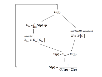
Figure 1: Schematic representation of the BDMC+DMFT protocol (see text for the details).

In this Letter, we show that, in addition to simply going from bare to skeleton expansion, a dramatic increase in performance can be reached by employing an exact series re-summation procedure which accounts for the summation of all local contributions to the self-energy. This approach amounts to embedding the dynamic mean-field theory (DMFT)DMFT1 solution into an exact diagrammatic method and avoids, in particular, any double counting or other uncontrollable errors. The gain in efficiency comes from two related observations: an impressive success of DMFT applications DMFT1 ; DMFT2 , and the fact that summation of local contributions can be done separately by a variety of highly efficient methods. The BDMC+DMFT approach thus involves two distinct but cross-linked numerical processes: (i) a problem-specific solver of the DMFT-type problem (to be referred to as ‘impurity solver’, in accordance with terminology accepted in literature), and (ii) a generic BDMC scheme simulating skeleton diagrams which cannot be reduced to the purely local ones. The protocol is illustrated in Fig. 1.

Below we start with the precise formulation of the combined scheme, and then proceed with its implementation for finding a disorder-averaged single-particle propagator (and thus the density of states) in the non-perturbative regime of the Anderson localization problem which is well suited for illustrating the idea because the efficiency gained by incorporating DMFT solutions within the BDMC is about $10^{4}$. In general, the gain will be problem and parameter specific, and will also depend on the efficiency of the impurity solver. [We stress that our goal in this article is to explain the new method and illustrate its implementation, not to solve the localization problem in its full complexity.]

Formalism. – The protocol of reformulating skeleton series to account for all local contributions to self-energy is conceptually straightforward. The Dyson equation relates the Green’s function, $G$, to the self-energy, $\Sigma$ (for clarity, we suppress below the frequency variable):

$$G({\mathbf{p}})\,=\,\frac{1}{G_{0}^{-1}({\mathbf{p}})-\Sigma({\mathbf{p}})}\,,$$ (1)

with $G_{0}$ standing for the non-perturbed Green’s function. The local propagator $G_{\rm loc}$ is defined by integrating over the Brillouin zone ‘BZ’

$$G_{\rm loc}\,=\,\int_{\rm BZ}\,G({\mathbf{p}})\,\frac{d{\mathbf{p}}}{(2\pi)^{d}}\;.$$ (2)

We now separate contributions to the self-energy into two parts

$$\Sigma({\mathbf{p}})=\Sigma_{\rm loc}+\Sigma^{\prime}({\mathbf{p}})\;,$$ (3)

where $\Sigma_{\rm loc}$ is given by irreducible skeleton diagrams which involve exclusively $G_{\rm loc}$ propagators. In other words, this local propagator has only purely momentum independent building blocks, while all the rest is put in $\Sigma^{\prime}$.

Numerically, one calculates the self-energy using current knowledge of the Green’s function and then uses it to permanently improve the knowledge of $G$ within the self-consistent process. This involves two steps. First, the current knowledge of $G_{\rm loc}$ serves as an input for the calculation of $\Sigma_{\rm loc}\equiv\Sigma_{\rm loc}[G_{\rm loc}]$ achieved by the impurity solver, and $G({\mathbf{p}})$ is used for the BDMC simulation of the remaining skeleton graphs. Second, self-energies $\Sigma_{\rm loc}$ and $\Sigma^{\prime}$ are combined into the total self-energy, Eq. (3), which is then used to find the updated $G$ by Eq. (1). This is illustrated in Fig. 1.

Technically, the crucial advantage of separating local contributions to the self-energy is that the corresponding momentum independent problem admits a variety of techniques for solving it very efficiently impurity_solvers . Treating the local physics non-perturbatively is very appealing from the physical viewpoint. In typical problems such as the Hubbard model, the diagrammatic technique expands around the non-interacting limit which is dominated by large hopping processes. The competing phase with large on-site interactions tends on the contrary to localize the particles. Hence, building diagrams on top of the solution capturing essential physics of the competing phase may be better suited for describing the difficult intermediate regime as well. Local physics is also dominant at high temperatures which can easily be understood in terms of Feynman’s path integrals.

From Eqs. (1)-(2) it is explicitly seen that BDMC+DMFT process builds an exact solution of the problem on top of the DMFT answer, which is crucial not only for improving the quality of the final result but also for reliable estimates of corrections to mean-field results.

One of the solvers for obtaining $\Sigma_{\rm loc}$ in terms of $G_{\rm loc}$ widely used in the standard DMFT approach is based on an implicit formulation of the problem in terms of the single-site (or impurity) effective action with a certain auxiliary (to be determined) ‘bare” propagator $\tilde{g}_{0}$. The advantage of this formulation is in the flexibility of designing efficient tools (impurity solvers) impurity_solvers for obtaining the $G_{\rm loc}[\tilde{g}_{0}]$ relation; the local self-energy readily follows from $\Sigma_{\rm loc}=\tilde{g}_{0}^{-1}-G_{\rm loc}^{-1}$. Iterations leading to the self-consistent solution consist of plugging the thus obtained self-energy in Eq. (2) to redefine the auxiliary propagator by $\tilde{g}_{0}^{-1}=G_{\rm loc}^{-1}[\Sigma]+\Sigma_{\rm loc}$. Solvers based on the effective action approach play a crucial part when the diagrammatic expansion of $\Sigma_{\rm loc}[G_{\rm loc}]$ cannot be used because of technical or convergence problems.

Illustration. – We illustrate the introduced concepts for Anderson’s model of particle localization on a disordered three-dimensional cubic lattice. We consider delta-correlated gaussian disorder in the chemical potential, for which the standard diagrammatic technique can be formulated AGD . The Hamiltonian, in standard lattice notation, reads

$$H=-J\sum_{\langle i,j\rangle}\,\hat{c}_{i}^{\dagger}\hat{c}_{j}\,+\,\sum_{i}\,\epsilon_{i}\,\hat{n}_{i}\,.$$ (4)

The random on-site potential $\epsilon_{i}$ is distributed with the gaussian probability density

$$P(\epsilon)=\frac{e^{-\epsilon^{2}/2V^{2}}}{\sqrt{2\pi V^{2}}}\,,$$ (5)

the dispersion $V$ characterizing the strength of the disorder. We choose $J=1$ as our unit. We work in the real-time representation where the Green function is defined as $G({\bf r},t^{\prime}\!-\!t)=-i\,\langle\,{\mathcal{T}}c(0,t)\,c^{\dagger}({\bf r},t^{\prime})\,\rangle$. We took a lattice of size $12\times 12\times 12$. Just like in conventional DMFT, larger lattices pose no problem at all; in fact, larger lattices would suppress revivals and make hence the simulations easier. The (local) density of states is given by the imaginary part of its Fourier transform for ${\bf r}=0$, ${\rm DOS}(\omega)=-\pi^{-1}{\rm Im}G({\bf r}=0,\omega)$, which can be compared with the exact diagonalizaton results of Refs. Kravtsov ; Wortis .

Evaluating the sum of all skeleton diagrams involviong local propagators only (i.e., the DMFT part Byczuk10 ) simplifies for Anderson’s localization since disorder lines have no time dependence. For a single-site problem, one does not even need to expand the gaussian exponential into the diagrammatic series, because averaging the Green’s function—in the frequency representation, the former is immediately found to be equal to $1/[1/\tilde{g}_{0}(\omega)-i\epsilon]$—over the disorder amounts to performing a simple one-dimensional integral:

$$G_{\rm loc}(\omega)=\frac{\tilde{g}_{0}(\omega)}{\sqrt{2\pi V^{2}}}\int\frac{e^{-\epsilon^{2}/2V^{2}}}{1-i\epsilon\tilde{g}_{0}(\omega)}\,d\epsilon\;.$$ (6)

The local self-energy then follows from $\Sigma_{\rm loc}(\omega)=\tilde{g}_{0}^{-1}(\omega)-G_{\rm loc}^{-1}(\omega)$ which accounts for the implicit (parametric) complex-number relation $\Sigma_{\rm loc}[G_{\rm loc}]$, i.e. the goal is achieved by the semi-analytic exact solution. In practice this is done by a parametrization of the above integral equation through $\tilde{g}_{0}[G_{\rm loc}]$ (inversion), and iterating until self-consistency is reached. This works fine here only because the interaction lines carry no time dependence. In Fig. 2 we show for various disorder strengths the local self-energy obtained for $\Sigma^{\prime}=0$ after convergence, i.e. the answer as predicted by the conventional DMFT approach.

The full calculation involves Monte Carlo sampling of all skeleton diagrams except those contributing to $\Sigma_{\rm loc}$ (which would otherwise consume about $90\%$ of the simulation time already for $V=\sqrt{2}$). In the real-space representation this means that only skeleton graphs which contain at least two vertices with different site indices are accounted for in $\Sigma^{\prime}$. The simulation itself was done using standard BDMC rules with the self-consistency loop implemented exactly as described in the introductory part of this Letter. It turns out that the diagrammatic series for Anderson’s localization problem constitutes the ‘worst case scenario’ in terms of convergence properties. Although for any finite time $t$ the series are convergent (allowing us to use Dyson’s equation and Eq. (6)), the required expansion order increases dramatically with the time $t$. Realistically, we were able to deal with skeleton graphs up to order $n_{\rm max}\sim 50$ which was limiting the accessible times in the simulation of $\Sigma^{\prime}$. We observe that the values of $\Sigma^{\prime}_{{\mathbf{r}}-{\mathbf{r}}^{\prime}}\equiv\Sigma^{\prime}_{\mathbf{n}}$ turn out to be extremely small, about two orders of magnitude smaller than $\Sigma_{\rm loc}$ even in the intermediate coupling regime $V=\sqrt{2}$, see Fig. 3. Since the complexity, and hence the relative error-bar, of the BDMC simulation is roughly the same for simulating $\Sigma$ or $\Sigma^{\prime}$, we conclude that the BDMC+DMFT scheme produces results which are two orders of magnitude (or a speedup of $\sim 10^{4}$ in CPU time) more accurate for the same simulation time in the region of parameter space where the series converges and error bars are under control. This constitutes the proof of principle for the proposed scheme. Final results for the density of states are indistinguishable from the exact diagonalization data.

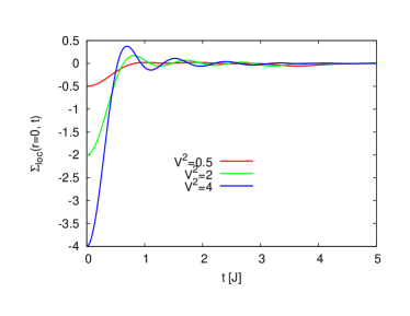
Figure 2: (Color online) Local self-energy calculated using local propagators ($\Sigma^{\prime}=0$) for disorder strengths $V=1/\sqrt{2},~{}\sqrt{2},~{}4$ on a lattice of size $12\times 12\times 12$.

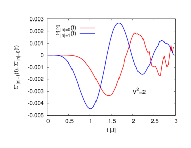
Figure 3: (Color online) Correction to local self-energy for $V=\sqrt{2}$ on a lattice of size $12\times 12\times 12$: $\Sigma^{\prime}_{|{\mathbf{n}}|=0}(t)$ (red line) and $\Sigma^{\prime}_{|{\mathbf{n}}|=1}(t)$ (blue line). The noise in the curve is indicative of the error bars. The sign problem and the high expansion orders put a limit on the accessible times.

Outlook and Conclusions. – We have introduced an approach that uses DMFT as an integral part of performing simulations of skeleton graphs in strongly interacting systems. It combines the power of solving impurity problems efficiently with the diagrammatic formalism that is unbiased and exact. Given the already good agreement between DMFT and diagrammatic Monte Carlo based on bare propagators for the Hubbard model at $U/J=4$ Kozik10 , we expect the present formalism to bring radical speed up and accuracy to studies of the Hubbard model at larger values of $U$ and lower temperatures.

We would also like to mention several generalizations of the simplest scheme introduced above. To begin with, the definition of momentum-independent propagator allows the use of an arbitrary function $f({\mathbf{p}})$ in the definition of $G_{\rm loc}$ such that $G_{\rm loc}=\int_{\rm BZ}\,G({\mathbf{p}})f({\mathbf{p}})\,d{\mathbf{p}}/(2\pi)^{d}$. The rest of the scheme remains intact: as before diagrams containing exclusively $G_{\rm loc}$ propagators are all summed up in the local self-energy while $\Sigma^{\prime}$ contains at least one line which is based on $G({\mathbf{p}})-G_{\rm loc}$. The freedom of choosing $f({\mathbf{p}})$ different from a constant may be used to optimize the subtraction of leading terms.

In the generic many-body skeleton diagram, any renormalized line whether it is the single-particle propagator $G({\mathbf{p}})$, the interaction line $W({\mathbf{q}})$, or the two-particle propagator $\Gamma$, can be split into momentum-independent and momentum-dependent parts (with the same freedom of defining the local part as described in the previous paragraph). Next, all diagrams based exclusively on momentum-independent lines can be dealt with using impurity solvers with BDMC accounting for the remaining graphs. Since the summation of certain geometric series such as ladder or screening diagrams can be done analytically to set up the original diagrammatic space, one can go even further beyond the purely local physics by doing so.

Our final remark is that nothing prevents one from extending the idea of subtracting diagrams with momentum-independent lines (and compensating them separately by impurity solvers) to subtracting diagrams with specific momentum-dependence and structure, (and compensating them by impurity solvers dealing with a few sites, similar to the ideas behind cluster-DMFT schemes). The diagrams to be summed up by the impurity solver are those with the connections of a compact cluster of sites. Similar extensions for real-space clusters are also possible.

This work was supported by the National Science Foundation grant PHY-1005543, the Swiss National Science Foundation under grant PZ00P2-131892/1, and by a grant from the Army Research Office with funding from the DARPA OLE program. We thank the Aspen Center of Physics, KITP Santa Barbara, and Casa Física at UMass for hospitality. Simulations were performed on the Brutus cluster at ETH Zurich and CM cluster at UMass, Amherst.

References

- (1) N. Prokof’ev, and B. Svistunov, Phys. Rev. Lett. 99, 250201 (2007); Phys. Rev. B 77, 125101 (2008).
- (2) K. Van Houcke, E. Kozik, N. Prokof’ev, and B. Svistunov, Diagrammatic Monte Carlo, [in Computer Simulation Studies in Condensed Matter Physics XXI, Eds. D.P. Landau, S.P. Lewis, and H.B. Schuttler (Springer Verlag, Heidelberg, Berlin 2008)], arXiv:0802.2923.
- (3) E. Kozik, K. Van Houcke, E. Gull, L. Pollet, N. Prokof’ev, B. Svistunov, and M. Troyer, Europhys. Lett. 90, 10004 (2010).
- (4) K. Van Houcke, et al. , in preparation.
- (5) A. Georges, G. Kotliar, W. Krauth, and M. J. Rozenberg, Rev. Mod. Phys. 68, 13 (1996).
- (6) G. Kotliar, S. Y. Savrasov, K. Haule, V. S. Oudovenko, O. Parcollet, and C. A. Marianetti, Rev. Mod. Phys. 78, 865 (2006).
- (7) E. Gull, A. J. Millis, A. I. Lichtenstein, A. N. Rubtsov, M. Troyer, and P. Werner, arXiv:1012:4474, to appear in Rev. Mod. Phys. (2010).
- (8) A. A. Abrikosov, L. P. Gor’kov, and I. E. Dzyaloshinski, Methods of Quantum Field Theory in Statistical Physics, Dover Publications Inc. (1975).
- (9) M. V. Feigel’man, L. B. Ioffe, V. E. Kravtsov, and E. Cuevas, Annals of Physics 325, 1368 (2010).
- (10) K. Byczuk, W. Hofstetter, and D. Vollhardt, in ”50 Years of Anderson Localization”, ed. E. Abrahams (World Scientific, Singapore, 2010), p. 473; reprinted in Int. J. Mod. Phys. B 24, 1727 (2010).
- (11) N. C. Murphy, R. Wortis, and W. A. Atkinson, arXiv:1011.0659 (2010).