High order weak approximation schemes for Lévy-driven SDEs

Abstract

We propose new jump-adapted weak approximation schemes for stochastic differential equations driven by pure-jump Lévy processes. The idea is to replace the driving Lévy process $Z$ with a finite intensity process which has the same Lévy measure outside a neighborhood of zero and matches a given number of moments of $Z$. By matching 3 moments we construct a scheme which works for all Lévy measures and is superior to the existing approaches both in terms of convergence rates and easiness of implementation. In the case of Lévy processes with stable-like behavior of small jumps, we construct schemes with arbitrarily high rates of convergence by matching a sufficiently large number of moments.

Key words: Lévy-driven stochastic differential equation, Euler scheme, high order discretization schemes, jump-adapted discretization, weak approximation.

2010 Mathematics Subject Classification: Primary 60H35, Secondary 65C05, 60G51.

1 Introduction

Let $Z$ be a $d$-dimensional Lévy process without diffusion component, that is,

$$Z_{t}=\gamma t+\int_{0}^{t}\int_{|y|\leq 1}y\widehat{N}(dy,ds)+\int_{0}^{t}\int_{|y|>1}yN(dy,ds),\quad t\in[0,1].$$

Here $\gamma\in\mathbb{R}^{d}$, $N$ is a Poisson random measure on $\mathbb{R}^{d}\times[0,\infty)$ with intensity $\nu$ satisfying $\int 1\wedge\|y\|^{2}\nu(dy)<\infty$ and $\widehat{N}(dy,ds)=N(dy,ds)-\nu(dy)ds$ denotes the compensated version of $N$. We study the case when $\nu(\mathbb{R}^{d})=\infty$, that is, there is an infinite number of jumps in every interval of nonzero length a.s. Further, let $X$ be an $\mathbb{R}^{n}$-valued adapted stochastic process, unique solution of the stochastic differential equation

$$X_{t}=X_{0}+\int_{0}^{t}h(X_{s-})dZ_{s},\quad t\in[0,1],$$ (1)

where $h$ is an $m\times d$ matrix.

In this article we are interested in the numerical evaluation of $E[f(X_{1})]$ for a sufficiently smooth function $f$ by Monte Carlo, via discretization and simulation of the process $X$. We propose new weak approximation algorithms for (1) and study their rate of convergence.

The traditional method to simulate $X$ is to use the Euler scheme with constant time step

$$\hat{X}^{n}_{\frac{i+1}{n}}=\hat{X}^{n}_{\frac{i}{n}}+h(\hat{X}^{n}_{\frac{i}{n}})(Z_{\frac{i+1}{n}}-Z_{\frac{i}{n}}).$$

This method has the convergence rate [9, 6]

$$|E[f(X_{1})]-E[f(\hat{X}^{n}_{1})]|\leq\frac{C}{n}$$

but suffers from two difficulties: first, for a general Lévy measure $\nu$, there is no available algorithm to simulate the increments of the driving Lévy process and second, a large jump of $Z$ occurring between two discretization points can lead to an important discretization error.

A natural idea due to Rubenthaler [11] (in the context of finite-intensity jump processes, this idea appears also in [2, 8]), is to approximate $Z$ with a compound Poisson process by replacing the small jumps with their expectation

$$Z^{\varepsilon}_{t}:=\gamma_{\varepsilon}t+\int_{0}^{t}\int_{|y|>\varepsilon}yN(dy,ds),\quad\gamma_{\varepsilon}=\gamma-\int_{\varepsilon<|y|\leq 1}y\nu(dy),$$

and then place discretization dates at all jump times of $Z^{\varepsilon}$.

The computational complexity of simulating a single trajectory using this method becomes a random variable, but the convergence rate may be computed in terms of the expected number of discretization dates, proportional to $\lambda_{\varepsilon}=\int_{|y|\geq\varepsilon}\nu(dy)$. When the jumps of $Z$ are highly concentrated around zero, however, this approximation is too rough and the convergence rates can be arbitrarily slow.

In [7], the authors proposed a scheme which builds on Rubenthaler’s idea of using the times of large jumps of $Z$ as discretization dates but achieves better convergence rates. Their idea is, first, to approximate the small jumps of $Z$ with a suitably chosen Brownian motion, in order to match not only the first but also the second moment of $Z$, and second, to construct an approximation to the solution of the continuous SDE between the times of large jumps. Similar ideas of Gaussian correction were recently used in [5] in the context of multilevel Monte Carlo methods for the problem (1). However, although diffusion approximation of small jumps improves the convergence rate, there are limits on how well the small jumps of a Lévy process can be approximated by a Brownian motion. In particular, the Brownian motion is a symmetric process, while a Lévy process may be asymmetric.

In this paper we develop new jump-adapted discretization schemes based on approximating the Lévy process $Z$ with a finite intensity Lévy process $Z^{\varepsilon}$ without diffusion part. Contrary to previous works, instead of simply truncating jumps smaller than $\varepsilon$, we construct efficient finite intensity approximations which match a given number of moments of $Z$. These approximations are superior to the existing approaches in two ways. First, given that $Z^{\varepsilon}$ is a finite intensity Lévy process, the solution to (1) with $Z$ replaced by $Z^{\varepsilon}$ is easy to compute, either explicitly or with a fast numerical method, making it straightforward to implement the scheme. Second, by choosing the parameters of $Z^{\varepsilon}$ in a suitable manner, one can, in principle, match an arbitrary number of moments of $Z$ and obtain a discretization scheme with an arbitrarily high convergence rate.

The paper is structured as follows. In Section 2, we present the main idea of moment matching approximations and provide a basic error bound for such schemes. In Section 3, we introduce our first scheme which is based on matching 3 moments of $Z$ and can be used for general Lévy processes. For Lévy processes with stable-like behavior of small jumps near zero, the scheme is shown to be rate-optimal. Finally, Section 4 shows how schemes of arbitrary order can be constructed by matching additional moments, once again, in the context of Lévy processes with stable-like behavior of small jumps.

2 Moment matching compound Poisson approximations

Let $Z^{\varepsilon}$ be a finite intensity Lévy process without diffusion part approximating $Z$ in a certain sense to be defined later:

$$Z^{\varepsilon}_{t}:=\gamma_{\varepsilon}t+\int_{0}^{t}\int_{\mathbb{R}^{d}}yN^{\varepsilon}(dy,ds),$$ (2)

where $N^{\varepsilon}$ is a Poisson random measure with intensity measure $dt\times\nu^{\varepsilon}$ such that $\lambda_{\varepsilon}:=\nu^{\varepsilon}(\mathbb{R}^{d})<\infty$.

In this paper we propose to approximate the process (1) by the solution to

$$d\hat{X}_{t}=h(\hat{X}_{t-})dZ^{\varepsilon}_{t},\quad\hat{X}_{0}=X_{0},$$ (3)

which can be computed by applying the Euler scheme at the jump times of $Z^{\varepsilon}$ and solving the deterministic ODE $d\hat{X}_{t}=h(\hat{X}_{t})\gamma_{\varepsilon}dt$ explicitly (or by a Runge-Kutta method) between these jump times. The following proposition provides a basic estimate for the weak error of such an approximation scheme. We impose the following alternative regularity assumptions on the functions $f$ and $h$:

$\mathbf{(H_{n})}$

$f\in C^{n}$, $h\in C^{n}$ $f^{(k)}$ and $h^{(k)}$ are bounded for $1\leq k\leq n$ and $\int z^{2n}\nu(dz)<\infty$.

$\mathbf{(H^{\prime}_{n})}$

$f\in C^{n}$, $h\in C^{n}$, $h^{(k)}$ are bounded for $1\leq k\leq n$, $f^{(k)}$ have at most polynomial growth for $1\leq k\leq n$ and $\int|z|^{k}\nu(dz)<\infty$ for all $k\geq 1$.

Proposition 1.

Let $Z$ and $\hat{Z}$ be Lévy processes with characteristic triplets $(0,\nu,\gamma)$ and $(0,\hat{\nu},\hat{\gamma})$ respectively, and let $X$ and $\hat{X}$ be the corresponding solutions of SDE (1). Assume $\hat{\gamma}=\gamma$, $\hat{\nu}=\nu$ on $\{\|x\|>1\}$, either $\mathbf{(H_{n})}$ or $\mathbf{(H^{\prime}_{n})}$ for $n\geq 3$ and

$$\int_{\mathbb{R}^{d}}x_{i_{1}}\dots x_{i_{k}}\nu(dx)=\int_{\mathbb{R}^{d}}x_{i_{1}}\dots x_{i_{k}}\hat{\nu}(dx),\quad 2\leq k\leq n-1,\quad 1\leq i_{k}\leq d.$$ (4)

Then

$$|E[f(\hat{X}_{1})-f(X_{1})]|\leq C\int_{\mathbb{R}^{d}}\|x\|^{n}|d\nu-d\hat{\nu}|,$$

where the constant $C$ may depend on $f$, $g$, $x$ and $\nu$ but not on $\hat{\nu}$.

Proof.

To simplify notation, we give the proof in the case $m=d=1$. Let $u(t,x)=E^{(t,x)}[f(X_{1})]$. By Lemma 13 in [7], $u\in C^{1,n}([0,1]\times\mathbb{R})$ and satisfies

$$\frac{\partial u}{\partial t}(t,x) +\gamma\frac{\partial u}{\partial x}(t,x)h(x)+\int_{|y|>1}\left(u(t,x+h(x)y)-u(t,x)\right)\nu\left(dy\right)$$

$$+\int_{|y|\leq 1}\left(u(t,x+h(x)y)-u(t,x)-\frac{\partial u}{\partial x}(t,x)h(x)y\right)\nu(dy)=0,$$ (5)

$$u(1,x) =f(x).$$

Applying Itô formula under the integral sign and using (5) and Lemma 11 in [7] (bounds on moments of $\hat{X}_{t}$) yields

$$E[f(\hat{X}_{1})-f(X_{1})]=E[u(1,\hat{X}_{1})-u(0,X_{0})]$$

$$=E\left[\int_{0}^{1}\int_{\mathbb{R}}\left\{u(t,\hat{X}_{t}+h(\hat{X}_{t})z)-u(t,\hat{X}_{t})-h(\hat{X}_{t})z\frac{\partial u}{\partial x}\right\}(d\nu_{\varepsilon}-d\nu)dt\right]$$

$$+E\left[\int_{0}^{1}\int_{\mathbb{R}}\left\{u(t,\hat{X}_{t-}+h(\hat{X}_{t-})z)-u(t,\hat{X}_{t-})\right\}\hat{N}(dz,dt)\right]$$

$$=E\left[\int_{0}^{1}\int_{\mathbb{R}}\sum_{k=2}^{n-1}\frac{\partial^{k}u(t,\hat{X}_{t})}{\partial x^{k}}h^{k}(\hat{X}_{t})z^{k}(d\nu_{\varepsilon}-d\nu)dt+\text{remainder}\right],$$

$$=E[\text{remainder}],$$

where in the last line we used the moment matching condition (17) and the remainder coming from the Taylor formula can be estimated as

$$|\text{remainder}| \leq\int_{0}^{1}\int_{\mathbb{R}}\sup_{0\leq s\leq 1}\left|\frac{\partial^{n}u(s,\hat{X}_{s})}{\partial x^{n}}\right||h(\hat{X}_{t})|^{n}|z|^{n}|d\nu_{\varepsilon}-d\nu|dt$$

$$\leq C\sup_{0\leq s\leq 1}\left|\frac{\partial^{n}u(s,\hat{X}_{s})}{\partial x^{n}}\right|\sup_{0\leq s\leq 1}|h(\hat{X}_{s})|^{n}\int_{\mathbb{R}}|z|^{n}|d\nu_{\varepsilon}-d\nu|$$

From the Lipschitz property of $h$ and Lemma 13 in [7],

$$\sup_{0\leq s\leq 1}\left|\frac{\partial^{n}u(s,\hat{X}_{s})}{\partial x^{n}}\right|\sup_{0\leq s\leq 1}|h(\hat{X}_{s})|^{n}\leq C(1+\sup_{0\leq t\leq 1}|\hat{X}_{t}|^{p})$$

for some $C<\infty$, where $p=n$ under $\mathbf{(H_{n})}$ and $p>n$ under $\mathbf{(H^{\prime}_{n})}$. Following the arguments in the proof of Lemma 11 in [7], we get

$$E[\sup_{0\leq t\leq 1}|\hat{X}_{t}|^{p}]\leq C(1+|x|^{p})\exp\left[c\left(|\bar{\gamma}|^{p}+\int_{\mathbb{R}}|z|^{p}\hat{\nu}(dz)+\left(\int_{\mathbb{R}}z^{2}\hat{\nu}(dz)\right)^{p/2}\right)\right]$$

for different constants $C$ and $c$, where

$$\bar{\gamma}=\hat{\gamma}+\int_{|z|>1}z\hat{\nu}(dz)=\gamma+\int_{|z|>1}z\nu(dz)$$

by our assumptions. Since $\int_{\mathbb{R}}z^{2}\hat{\nu}(dz)=\int_{\mathbb{R}}z^{2}\nu(dz)$ by assumption, and

$$\int_{\mathbb{R}}|z|^{p}\hat{\nu}(dz)\leq\int_{|z|>1}|z|^{p}\hat{\nu}(dz)+\int_{|z|\leq 1}|z|^{2}\hat{\nu}(dz)=\int_{|z|>1}|z|^{p}\nu(dz)+\int_{|z|\leq 1}|z|^{2}\nu(dz),$$

it is clear that $E[\sup_{0\leq t\leq 1}|\hat{X}_{t}|^{p}]\leq C$ for some constant $C$ which does not depend on $\hat{\nu}$.

∎

3 The 3-moment scheme

Our first scheme is based on matching the first 3 moments of the process $Z$. Let $S^{d-1}$ be the unit sphere in the $d$-dimensional space, and $\nu(dr\times d\theta)$ be a Lévy measure on $\mathbb{R}^{d}$ written in spherical coordinates $r\in[0,\infty)$ and $\theta\in S^{d-1}$ and satisfying $\int_{[0,\infty)\times S^{d-1}}r^{3}\nu(dr,d\theta)<\infty$. Denote by $\bar{\nu}$ the reflection of $\nu$ with respect to the origin defined by $\bar{\nu}(B)=\nu(\{x:-x\in B\})$. We introduce two measures on $S^{d-1}$:

$$\bar{\lambda}(d\theta) =\frac{1}{2}\int_{|r|\leq\varepsilon}\frac{r^{3}}{\varepsilon^{3}}\left(\nu(dr,d\theta)-\bar{\nu}(dr,d\theta)\right)$$

$$\lambda(d\theta) =\frac{1}{2}\int_{|r|\leq\varepsilon}\frac{r^{2}}{\varepsilon^{2}}\left(\nu(dr,d\theta)+\bar{\nu}(dr,d\theta)\right).$$

The 3-moment scheme is defined by

$$\nu_{\varepsilon}(dr,d\theta) =\nu(dr,d\theta)1_{r>\varepsilon}+\delta_{\varepsilon}(dr)\{\lambda(d\theta)+\bar{\lambda}(d\theta)\}$$ (6)

$$\gamma_{\varepsilon} =\gamma-\int_{[0,1]\times S^{d-1}}r\theta\,\nu_{\varepsilon}(dr,d\theta),$$ (7)

where $\delta_{\varepsilon}$ denotes a point mass at $\varepsilon$.

Proposition 2 (Multidimensional 3-moment scheme).

For every $\varepsilon>0$, $\nu_{\varepsilon}$ is a finite positive measure satisfying

$$\int_{\mathbb{R}^{d}}x_{i}x_{j}\nu(dx) =\int_{\mathbb{R}^{d}}x_{i}x_{j}\nu_{\varepsilon}(dx)$$ (8)

$$\int_{\mathbb{R}^{d}}x_{i}x_{j}x_{k}\nu(dx) =\int_{\mathbb{R}^{d}}x_{i}x_{j}x_{k}\nu_{\varepsilon}(dx),\quad 1\leq i,j,k\leq d$$ (9)

$$\lambda_{\varepsilon}:=\int_{\mathbb{R}^{d}}\nu_{\varepsilon}(dx) =\int_{\|x\|>\varepsilon}\nu(dx)+\varepsilon^{-2}\int_{\|x\|\leq\varepsilon}\|x\|^{2}\nu(dx)$$ (10)

$$\int_{\mathbb{R}^{d}}\|x\|^{4}|d\nu-d\nu_{\varepsilon}|\leq \int_{\|x\|\leq\varepsilon}\|x\|^{4}\nu(dx)+\varepsilon^{2}\int_{\|x\|\leq\varepsilon}\|x\|^{2}\nu(dx),$$ (11)

where the last inequality is an equality if $\nu(\{x:\|x\|=\varepsilon\})=0$.

Proof.

The positivity of $\nu_{\varepsilon}$ being straightforward, let us check (8). Let $\{e_{i}\}_{i=1}^{d}$ be the coordinate vectors. Then,

$$\int_{\mathbb{R}^{d}}x_{i}x_{j}\nu_{\varepsilon}(dx)=\int_{[0,\infty)\times S^{d-1}}r^{2}\langle\theta,e_{i}\rangle\langle\theta,e_{j}\rangle\nu_{\varepsilon}(dr,d\theta)$$

$$=\int_{(\varepsilon,\infty)\times S^{d-1}}r^{2}\langle\theta,e_{i}\rangle\langle\theta,e_{j}\rangle\nu(dr,d\theta)+\int_{S^{d-1}}\varepsilon^{2}\langle\theta,e_{i}\rangle\langle\theta,e_{j}\rangle\{\lambda(d\theta)+\bar{\lambda}(d\theta)\}$$

$$=\int_{(\varepsilon,\infty)\times S^{d-1}}r^{2}\langle\theta,e_{i}\rangle\langle\theta,e_{j}\rangle\nu(dr,d\theta)+\int_{S^{d-1}}\varepsilon^{2}\langle\theta,e_{i}\rangle\langle\theta,e_{j}\rangle\lambda(d\theta)$$

$$=\int_{(0,\infty)\times S^{d-1}}r^{2}\langle\theta,e_{i}\rangle\langle\theta,e_{j}\rangle\nu(dr,d\theta)=\int_{\mathbb{R}^{d}}x_{i}x_{j}\nu(dx).$$

The other equations can be checked in a similar manner. ∎

Corollary 1.

Let $d=1$. Then the 3-moment scheme can be written as

$$\nu_{\varepsilon}(dx) =\nu(dx)1_{|x|>\varepsilon}+\lambda_{+}\delta_{\varepsilon}(dx)+\lambda_{-}\delta_{-\varepsilon}(dx)$$

$$\lambda_{\pm} =\frac{1}{2}\left\{\int_{|x|\leq\varepsilon}\frac{x^{2}}{\varepsilon^{2}}\nu(dx)\pm\int_{|x|\leq\varepsilon}\frac{x^{3}}{\varepsilon^{3}}\nu(dx)\right\}$$

Corollary 2 (Worst-case convergence rate).

Assume $\mathbf{(H_{4})}$ or $\mathbf{(H^{\prime}_{4})}$. Then the solution $\hat{X}$ of (3) with the characteristics of $Z^{\varepsilon}$ given by (6)–(7) satisfies

$$|E[f(\hat{X}_{1})-f(X_{1})]|=o(\lambda_{\varepsilon}^{-1}).$$

as $\varepsilon\to 0$.

Proof.

By Proposition 1 we need to show that

$$\lim_{\varepsilon\downarrow 0}\lambda_{\varepsilon}\int_{\mathbb{R}^{d}}\|x\|^{4}|d\nu-d\nu_{\varepsilon}|=0.$$

By Proposition 2,

$$\lim_{\varepsilon\downarrow 0}\lambda_{\varepsilon}\int_{\mathbb{R}^{d}}\|x\|^{4}|d\nu-d\nu_{\varepsilon}|$$

$$\leq\lim_{\varepsilon\downarrow 0}\left\{\int_{\|x\|>\varepsilon}\nu(dx)+\varepsilon^{-2}\int_{\|x\|\leq\varepsilon}\|x\|^{2}\nu(dx)\right\}$$

$$\qquad\qquad\times\left\{\int_{\|x\|\leq\varepsilon}\|x\|^{4}\nu(dx)+\varepsilon^{2}\int_{\|x\|\leq\varepsilon}\|x\|^{2}\nu(dx)\right\}$$

$$\leq 2\lim_{\varepsilon\downarrow 0}\varepsilon^{2}\left\{\int_{\|x\|>\varepsilon}\nu(dx)+\varepsilon^{-2}\int_{\|x\|\leq\varepsilon}\|x\|^{2}\nu(dx)\right\}\int_{\|x\|\leq\varepsilon}\|x\|^{2}\nu(dx)$$

$$=2\lim_{\varepsilon\downarrow 0}\varepsilon^{2}\int_{\|x\|>\varepsilon}\nu(dx)\int_{\|x\|\leq\varepsilon}\|x\|^{2}\nu(dx)$$

$$\leq 2\int_{\mathbb{R}^{d}}\|x\|^{2}\nu(dx)\lim_{\varepsilon\downarrow 0}\varepsilon^{2}\int_{\|x\|>\varepsilon}\nu(dx)=0,$$

where in the last line the dominated convergence theorem was used. ∎

In many parametric or semiparametric models, the Lévy measure has a singularity of type $\frac{1}{|x|^{1+\alpha}}$ near zero. This is the case for stable processes, tempered stable processes [10], normal inverse Gaussian process [1], CGMY [3] and other models. Stable-like behavior of small jumps is a standard assumption for the analysis of asymptotic behavior of Lévy processes in many contexts, and in our problem as well, this property allows to obtain a more precise estimate of the convergence rate. We shall impose the following assumption, which does not require the Lévy measure to have a density:

$\mathbf{(H-\alpha)}$

There exist $C>0$ and $\alpha\in(0,2)$ such that

$$l(r)\sim Cr^{-\alpha}\quad\text{as}\quad r\to 0$$ (12)

where $l(r):=\int_{\|x\|>r}\nu(dx)$.

Corollary 3 (Stable-like behavior).

Assume $\mathbf{(H-\alpha)}$ and $\mathbf{(H_{4})}$ or $\mathbf{(H^{\prime}_{4})}$. Then the solution $\hat{X}$ of (3) with the characteristics of $Z^{\varepsilon}$ given by (6)–(7) satisfies

$$|E[f(\hat{X}_{1})-f(X_{1})]|=O\left(\lambda_{\varepsilon}^{1-\frac{4}{\alpha}}\right).$$

Proof.

Under $\mathbf{(H-\alpha)}$, by integration parts we get that for all $n\geq 2$,

$$\int_{\|x\|\leq r}\|x\|^{n}\nu(dx)\sim\frac{C\alpha}{n-\alpha}r^{n-\alpha}\quad\text{as $r\to 0$.}$$

Therefore, under this assumption,

$$\lambda_{\varepsilon}\sim\frac{2C}{2-\alpha}\varepsilon^{-\alpha}\quad\text{and}\quad\int_{\mathbb{R}^{d}}\|x\|^{4}|d\nu-d\nu_{\varepsilon}|\lesssim\frac{C\alpha(6-2\alpha)}{(2-\alpha)(4-\alpha)}\varepsilon^{4-\alpha}\quad\text{as $\varepsilon\to 0$,}$$

from which the result follows directly. ∎

Rate-optimality of the 3-moment scheme

From Proposition 1 we know that under the assumption $\mathbf{(H_{4})}$ or $\mathbf{(H^{\prime}_{4})}$, the approximation error of a scheme of the form (2)–(3) can be measured in terms of the $4$-th absolute moment of the difference of Lévy measures. We introduce the class of Lévy measures on $\mathbb{R}^{d}$ with intensity bounded by $N$:

$$\mathcal{M}^{N}=\{\nu\ \text{L\'{e}vy measure on $\mathbb{R}^{d}$,}\ \nu(\mathbb{R}^{d})\leq N\}.$$

The class of Lévy measures with intensity bounded by $\lambda_{\varepsilon}$ is then denoted by $\mathcal{M}^{\lambda_{\varepsilon}}$, and the smallest possible error achieved by any measure within this class is bounded from below by a constant times $\inf_{\nu^{\prime}\in\mathcal{M}^{\lambda_{\varepsilon}}}\int_{\mathbb{R}^{d}}\|x\|^{4}|d\nu-d\nu^{\prime}|$. The next result shows that as $\varepsilon\to 0$, the error achieved by the 3-moment scheme $\nu_{\varepsilon}$ differs from this lower bound by at most a constant multiplicative factor .

Proposition 3.

Assume $\mathbf{(H-\alpha)}$ and let $\nu_{\varepsilon}$ be given by (6). Then,

$$\limsup_{\varepsilon\downarrow 0}\frac{\int_{\mathbb{R}^{d}}\|x\|^{4}|d\nu-d\nu_{\varepsilon}|}{\inf_{\nu^{\prime}\in\mathcal{M}^{\lambda_{\varepsilon}}}\int_{\mathbb{R}^{d}}\|x\|^{4}|d\nu-d\nu^{\prime}|}<\infty.$$

Proof.

Step 1. Let us first compute

$$\mathcal{E}_{N}:=\inf_{\nu^{\prime}\in\mathcal{M}^{N}}\int_{\mathbb{R}^{d}}\|x\|^{4}|d\nu-d\nu^{\prime}|.$$ (13)

For $\nu^{\prime}\in\mathcal{M}^{N}$, let $\nu^{\prime}=\nu^{\prime}_{c}+\nu^{\prime}_{s}$ where $\nu^{\prime}_{c}$ is absolutely continuous with respect to $\nu$ and $\nu^{\prime}_{s}$ is singular. Then $\nu^{\prime}_{c}(\mathbb{R}^{d})\leq N$ and

$$\int_{\mathbb{R}^{d}}\|x\|^{4}|d\nu-d\nu^{\prime}|=\int_{\mathbb{R}^{d}}\|x\|^{4}|d\nu-d\nu^{\prime}_{c}|+\int_{\mathbb{R}^{d}}\|x\|^{4}d\nu^{\prime}_{s}.$$

Therefore, the minimization in (13) can be restricted to measures $\nu^{\prime}$ which are absolutely continuous with respect to $\nu$, or, in other words,

$$\mathcal{E}_{N}=\inf\int_{\mathbb{R}^{d}}\|x\|^{4}|1-\lambda(x)|\nu(dx),$$

where the $\inf$ is taken over all measurable functions $\lambda:\mathbb{R}^{d}\to\mathbb{R}^{+}$ such that $\int_{\mathbb{R}^{d}}\lambda(x)\nu(dx)\leq N$. By a similar argument, one can show that it is sufficient to consider only functions $\lambda:\mathbb{R}^{d}\to[0,1]$. Given such a function $\lambda(r,\theta)$, the spherically symmetric function

$$\hat{\lambda}(r):=\frac{\int_{S^{d-1}}\lambda(r,\theta)\nu(dr,d\theta)}{\int_{S^{d-1}}\nu(dr,d\theta)}$$

leads to the same values of the intensity and the minimization functional. Therefore, letting $\hat{\nu}(dr):=\int_{S^{d-1}}\nu(dr,d\theta)$,

$$\mathcal{E}_{N}=\inf_{0\leq\hat{\lambda}\leq 1}\int_{0}^{\infty}r^{4}(1-\hat{\lambda}(r))\hat{\nu}(dr)\quad\text{s.~{}t.}\quad\int_{0}^{\infty}\hat{\lambda}(r)\hat{\nu}(dr)\leq N.$$ (14)

For every $e>0$,

$$\mathcal{E}_{N}\geq\inf_{0\leq\hat{\lambda}\leq 1}\left\{\int_{0}^{\infty}r^{4}(1-\hat{\lambda}(r))\hat{\nu}(dr)+e^{4}\left(\int_{0}^{\infty}\hat{\lambda}(r)\hat{\nu}(dr)-N\right)\right\}.$$

The $\inf$ in the right-hand side can be computed pointwise and is attained by $\hat{\lambda}(r)=1_{r>e}+\mu 1_{r=e}$ for any $\mu\in[0,1]$. Let $e(N)$ and $\mu(N)$ be such that

$$\hat{\nu}((e(N),\infty))+\mu(N)\hat{\nu}(\{e(N)\})=N.$$

Such a $e(N)$ can always be determined uniquely and $\mu(N)$ is determined uniquely if $\nu(\{e(N)\})>0$. It follows that $\hat{\lambda}(r)=1_{r>e(N)}+\mu(N)1_{r=e(N)}$ is a minimizer for (14) and therefore

$$\mathcal{E}_{N}=\int_{\|x\|<e}\|x\|^{4}\nu(dx)+(1-\mu)e^{4}\nu(\{x:\|x\|=e\}),$$

where $e$ and $\mu$ are solutions of

$$\nu(\{x:\|x\|>e\})+\mu\nu(\{x:\|x\|=e\})=N.$$

Step 2. For every $\varepsilon>0$, let $e(\varepsilon)$ and $\mu(\varepsilon)$ be solutions of

$$\nu(\{x:\|x\|>e(\varepsilon)\})+\mu(\varepsilon)\nu(\{x:\|x\|=e(\varepsilon)\})=\lambda_{\varepsilon}.$$

It is clear that $e(\varepsilon)\to 0$ as $\varepsilon\to 0$ and after some straightforward computations using the assumption $\mathbf{(H-\alpha)}$ we get that

$$\lim_{\varepsilon\to 0}\frac{e(\varepsilon)}{\varepsilon}=\left(\frac{2-\alpha}{2}\right)^{1/\alpha}.$$

Then,

$$\lim_{\varepsilon\downarrow 0}\frac{\int_{\mathbb{R}^{d}}\|x\|^{4}|d\nu-d\nu_{\varepsilon}|}{\mathcal{E}_{\lambda_{\varepsilon}}}=\lim_{\varepsilon\downarrow 0}\frac{\int_{\mathbb{R}^{d}}\|x\|^{4}|d\nu-d\nu_{\varepsilon}|}{\varepsilon^{4-\alpha}}\lim_{\varepsilon\downarrow 0}\frac{\varepsilon^{4-\alpha}}{e(\varepsilon)^{4-\alpha}}$$

$$\qquad\times\lim_{\varepsilon\downarrow 0}\frac{e(\varepsilon)^{4-\alpha}}{\int_{\|x\|<e(\varepsilon)}\|x\|^{4}\nu(dx)+(1-\mu(\varepsilon))e(\varepsilon)^{4}\nu(\{x:\|x\|=e(\varepsilon)\})}$$

Under $\mathbf{(H-\alpha)}$ the three limits are easily computed and we finally get

$$\lim_{\varepsilon\downarrow 0}\frac{\int_{\mathbb{R}^{d}}\|x\|^{4}|d\nu-d\nu_{\varepsilon}|}{\mathcal{E}_{\lambda_{\varepsilon}}}=(3-\alpha)\left(\frac{2}{2-\alpha}\right)^{4/\alpha}.$$ (15)

∎

Remark 1.

The constant $(3-\alpha)\left(\frac{2}{2-\alpha}\right)^{4/\alpha}>1$ appearing in the right-hand side of (15) cannot be interpreted as a “measure of suboptimality” of the 3-moment scheme, but only as a rough upper bound, because in the optimization problem (13) the moment-matching constraints were not imposed (if they were, it would not be possible to solve the problem explicitly). On the other hand, the fact that this constant is unbounded as $\alpha\to 2$ suggests that such a rate-optimality result cannot be shown for general Lévy measures without imposing the assumption $\mathbf{(H-\alpha)}$.

Numerical illustration

We shall now illustrate the theoretical results on a concrete example of a SDE driven by a normal inverse Gaussian (NIG) process [1], whose characteristic function is

$$\phi_{t}(u):=E[e^{iuZ_{t}}]=\exp\left\{-\delta t\left(\sqrt{\alpha^{2}-(\beta-iu)^{2}}-\sqrt{\alpha^{2}-\beta^{2}}\right)\right\},$$

where $\alpha>0$, $\beta\in(-\alpha,\alpha)$ and $\delta>0$ are parameters. The Lévy density is given by

$$\nu(x)=\frac{\delta\alpha}{\pi}\frac{e^{\beta x}K_{1}(\alpha|x|)}{|x|},$$

where $K$ is the modified Bessel function of the second kind. The NIG process has stable-like behavior of small jumps with $\nu(x)\sim\frac{const}{|x|^{2}}$, $x\to 0$ (which means that $\mathbf{(H-\alpha)}$ is satisfied with $\alpha=1$), and exponential tail decay. The increments of the NIG process can be simulated explicitly (see [4, algorithms 6.9 and 6.10]), which enables us to compare our jump-adapted algorithm with the classical Euler scheme.

For the numerical example we solve the one-dimensional SDE

$$dX_{t}=\sin(aX_{t})dZ_{t},$$

where $Z$ is the NIG Lévy process (with drift adjusted to have $E[Z_{t}]=0$). The solution of the corresponding deterministic ODE

$$dX_{t}=\sin(aX_{t})dt,\quad X_{0}=x$$

is given explicitly by

$$X_{t}=\theta(t;x)=\frac{1}{a}\arccos\frac{1+\cos(ax)-e^{2at}(1-\cos(ax))}{1+\cos(ax)+e^{2at}(1-\cos(ax))}$$

Figure 1 presents the approximation errors for evaluating the functional $E[(X_{1}-1)^{+}]$ by Monte-Carlo using the 3-moment scheme described in this section (marked with crosses), the diffusion approximation of [7] (circles) and the classical Euler scheme (diamonds). The parameter values are $\sigma=0.5$, $\theta=0.4$, $\kappa=0.6$, $a=5$ and $X_{0}=1$. For each scheme we plot the logarithm of the approximation error as function of the logarithm of the computational cost (time needed to simulate $10^{6}$ trajectories). The curves are obtained by varying the truncation parameter $\varepsilon$ for the two jump-adapted schemes and by varying the discretization time step for the Euler scheme.

The approximation error for the Euler scheme is a straight line with slope corresponding to the theoretical convergence rate of $\frac{1}{n}$. The graph for the 3-moment scheme seems to confirm the theoretical convergence rate of $\lambda_{\varepsilon}^{-3}$; the scheme is much faster than the other two and the corresponding curve quickly drops below the dotted line which symbolizes the level of the statistical error.

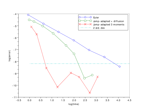
Figure 1: Approximation errors for the 3-moment scheme (crosses), the scheme of [7] (circles) and the Euler scheme (diamonds). The horizontal dotted line corresponds to the logarithm of the two standard deviations of the Monte Carlo estimator (the standard deviation is about the same for the three schemes and independent of the discretization step); everything that is below the dotted line is Monte Carlo noise.

4 High order schemes for stable-like Lévy processes

In this section, we develop schemes of arbitrary order for Lévy processes with stable-like behavior of small jumps. Throughout this section, we take $d=1$ and let $Z$ be a Lévy process with characteristic triplet $(0,\nu,\gamma)$ satisfying the following refined version of $\mathbf{(H-\alpha)}$:

$\mathbf{(H^{\prime}-\alpha)}$

There exist, $c_{+}\geq 0$, $c_{-}\geq 0$ with $c_{+}+c_{-}>0$ and $\alpha\in(0,2)$ such that

$$\int_{\varepsilon}^{\infty}\nu(dx)\sim c_{+}\varepsilon^{-\alpha}\quad\text{and}\quad\int_{-\infty}^{-\varepsilon}\nu(dx)\sim c_{-}\varepsilon^{-\alpha}\quad\text{as}\quad\varepsilon\downarrow 0$$

Introduce the probability measure

$$\mu^{*}(x):=\frac{(2-\alpha)|x|^{1-\alpha}(c_{+}1_{0\leq x\leq 1}+c_{-}1_{-1\leq x\leq 0})}{c_{+}+c_{-}}.$$ (16)

Let $n\geq 0$ and $\varepsilon>0$. The high-order scheme for the stochastic differential equation (1) based on $n+2$ moments and truncation level $\varepsilon$ is constructed as follows:

1. Find a discrete probability measure $\bar{\mu}=\sum_{i=0}^{n}a^{*}_{i}\delta_{x_{i}}$ with

   $$\int_{\mathbb{R}}x^{k}\bar{\mu}(dx)=\int_{\mathbb{R}}x^{k}\mu^{*}(dx),\quad 1\leq k\leq n,$$ (17)

   such that $x_{0}<x_{1}<\dots<x_{n}$, $x_{i}\neq 0$ for all $i$ and $a^{*}_{i}>0$ for all $i$.

2. Compute the coefficients $\{a^{\varepsilon}_{i}\}$ by solving the linear system

   $$\sigma^{2}_{\varepsilon}\sum_{i=0}^{n}a^{\varepsilon}_{i}x_{i}^{k}\varepsilon^{k}=\int_{|x|\leq\varepsilon}x^{2+k}\nu(dx),\ k=0,\dots,n,\ \sigma_{\varepsilon}^{2}=\int_{|x|\leq\varepsilon}x^{2}\nu(dx).$$

3. The high-order scheme is defined by

   $$\nu_{\varepsilon}(dx)=\nu(dx)1_{|x|>\varepsilon}+\sigma^{2}_{\varepsilon}\sum_{i=0}^{n}\frac{a^{\varepsilon}_{i}\delta_{\varepsilon x_{i}}(dx)}{x_{i}^{2}\varepsilon^{2}},\qquad\gamma_{\varepsilon}=\gamma-\int_{|z|\leq 1}z\nu_{\varepsilon}(dz).$$ (18)

Remark 2.

The first step in implementing the scheme is to solve the moment-matching problem (17) for measure $\mu^{*}$. The existence of at least one solution to this problem with $x_{0}<x_{1}<\dots x_{n}$ and $a^{*}_{i}\geq 0$ for all $i$ is guaranteed by the classical Caratheodory’s theorem, but this problem admits, in general, an infinite number of solutions. Here we impose the additional condition $x_{i}\neq 0$ and $a^{*}_{i}>0$ for all $i$, which should be checked on a case by case basis in concrete realizations of the scheme (see Example 1).

Remark 3.

It is easy to see that the measure

$$\nu^{*}_{\varepsilon}(dx):=(\sigma^{*}_{\varepsilon})^{2}\sum_{i=0}^{n}\frac{a^{*}_{i}\delta_{\varepsilon x_{i}}(dx)}{x_{i}^{2}\varepsilon^{2}},\quad(\sigma^{*}_{\varepsilon})^{2}:=\int_{|x|\leq\varepsilon}x^{2}\nu^{*}(z)dz.$$

matches the moments of orders $2,\dots,n+2$ of $\nu^{*}(x)1_{|x|\leq\varepsilon}$, where $\nu^{*}$ is the measure given by

$$\nu^{*}(x)=\frac{\alpha c_{+}1_{x>0}+\alpha c_{-}1_{x<0}}{|x|^{1+\alpha}},\quad$$

that is, $\nu^{*}$ satisfies the assumption $\mathbf{(H^{\prime}-\alpha)}$ with equalities instead of equivalences. The idea of the method is to replace the coefficients $\{a^{*}_{i}\}$ with a different set of coefficients while keeping the same points $\{x_{i}\}$ to obtain a measure which matches the moments of $\nu(x)1_{|x|\leq\varepsilon}$. Therefore, the points $\{x_{i}\}$ do not depend on the truncation parameter $\varepsilon$ while the coefficients $\{a^{\varepsilon}_{i}\}$ depend on it.

Example 1.

As an example we provide a possible solution of the moment matching problem for $n=3$, which leads to a 5-moment scheme (matching 3 moments of $\mu^{*}$ or $5$ moments of the Lévy process). We assume that $\mu^{*}$ has mass both on the positive and the negative half-line: $c_{+}c_{-}>0$.

The moments of $\mu^{*}$ are given by

$$m_{k}=\frac{2-\alpha}{k+2-\alpha}(\rho+(-1)^{k}(1-\rho)),\quad\rho:=\frac{c_{+}}{c_{+}+c_{-}}.$$

It is then convenient to look for the discrete measure matching the first 3 moments of $\mu^{*}$ in the form

$$\bar{\mu}=(1-\rho)(p\delta_{-\varepsilon_{2}}+(1-p)\delta_{-\varepsilon_{1}})+\rho((1-p)\delta_{\varepsilon_{1}}+p\delta_{\varepsilon_{2}}),$$ (19)

where $p\in(0,1)$, $0<\varepsilon_{1}<\varepsilon_{2}$ are parameters to be identified from the moment conditions

$$(1-p)\varepsilon_{1}^{k}+p\varepsilon_{2}^{k}=\frac{2-\alpha}{k+2-\alpha},\quad k=1,2,3.$$

For the purpose of solving this system of equations, let $\mathcal{E}$ be a random variable such that $P[\mathcal{E}=\varepsilon_{2}]=p=1-P[\mathcal{E}=\varepsilon_{1}]$. From the moment conditions, we get:

$$\bar{\varepsilon} :=E[\mathcal{E}]=\frac{2-\alpha}{3-\alpha},\qquad\sigma^{2}:=\text{Var}\,\mathcal{E}=\frac{(2-\alpha)}{(4-\alpha)(3-\alpha)^{2}},$$ (20)

$$s :=\frac{E[(\mathcal{E}-E[\mathcal{E}])^{3}]}{\sigma^{3}}=2\frac{\alpha-1}{5-\alpha}\sqrt{\frac{4-\alpha}{2-\alpha}}.$$ (21)

On the other hand, the skewness $s$ can be directly linked to the weight $p$:

$$s=\frac{1-2p}{\sqrt{p(1-p)}}\quad\Rightarrow\quad p=\frac{1}{2}-\frac{1}{2}\text{sign}\,(s)\sqrt{\frac{s^{2}}{s^{2}+4}},$$ (22)

and the parameters $\varepsilon_{1}$ and $\varepsilon_{2}$ can be linked to $\bar{\varepsilon},\sigma$ and $p$:

$$\varepsilon_{1}=\bar{\varepsilon}-\sigma\sqrt{\frac{p}{1-p}},\quad\varepsilon_{2}=\bar{\varepsilon}+\sigma\sqrt{\frac{1-p}{p}}.$$ (23)

The dependence of $\varepsilon_{1}$, $\varepsilon_{2}$ and $p$ on $\alpha$ is shown in Figure 2: it is clear from the graph that the constraints $p\in(0,1)$ and $0<\varepsilon_{1}<\varepsilon_{2}$ are satisfied for all $\alpha\in(0,2)$: therefore, equations (19–23) define a $4$-atom probability measure which matches the first 3 moments of $\mu^{*}$.

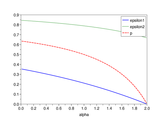
Figure 2: Solution of the moment matching problem for 3 moments (see Example 1).

Proposition 4.

Let $\{x_{i}\}$ be fixed according to (17). There exists $\varepsilon_{0}>0$ such that for all $\varepsilon<\varepsilon_{0}$, $\nu_{\varepsilon}$ is a positive measure satisfying

$$\int_{\mathbb{R}}x^{k}\nu(dx)=\int_{\mathbb{R}}x^{k}\nu_{\varepsilon}(dx),\quad 2\leq k\leq n+2$$ (24)

There exist positive constants $C_{1}$ and $C_{2}$ such that

$$\lambda_{\varepsilon}=\nu_{\varepsilon}(\mathbb{R})\sim C_{1}\varepsilon^{-\alpha},\qquad\int_{\mathbb{R}}|x|^{n+3}|d\nu-d\nu_{\varepsilon}|\lesssim C_{2}\varepsilon^{n+3-\alpha}\quad\text{as $\varepsilon\to 0$}.$$

Corollary 4.

Assume $(\mathbf{H_{n+3}})$ or $\mathbf{(H^{\prime}_{n+3})}$. Then the solution $\hat{X}$ of (3) with characteristics of $Z^{\varepsilon}$ given by (18) satisfies

$$|E[f(\hat{X}_{1})-f(X_{1})]|=O\left(\lambda_{\varepsilon}^{1-\frac{n+3}{\alpha}}\right).$$

of Proposition 4.

The moment conditions (24) hold by construction. Using integration by parts, we compute

$$\int_{|z|\leq\varepsilon}z^{2+k}\nu(dz)\sim\frac{(c_{+}+(-1)^{k}c_{-})\alpha\varepsilon^{2+k-\alpha}}{2+k-\alpha}\quad\text{as $\varepsilon\to 0$ for $k\geq 0$.}$$

Therefore,

$$\lim_{\varepsilon\to 0}\frac{1}{\sigma^{2}_{\varepsilon}\varepsilon^{k}}\int_{|z|\leq\varepsilon}z^{2+k}\nu(dz)=\frac{(2-\alpha)(c_{+}+(-1)^{k}c_{-})}{(2+k-\alpha)(c_{+}+c_{-})}=\int_{\mathbb{R}}x^{k}\mu^{*}(dx).$$

Since the matrix $M_{ij}=(x_{j})^{i}$, $0\leq i\leq n$, $0\leq j\leq n$ is invertible (Vandermonde matrix), this implies that $\lim_{\varepsilon\to 0}a^{\varepsilon}_{i}=a^{*}_{i}$. Therefore, there exists $\varepsilon_{0}>0$ such that for all $\varepsilon<\varepsilon_{0}$, $a^{\varepsilon}_{i}>0$ for all $i$ and $\nu_{\varepsilon}$ is a positive measure.

We next compute:

$$\nu_{\varepsilon}(\mathbb{R}) =\int_{|x|>\varepsilon}\nu(dx)+\frac{\sigma_{\varepsilon}^{2}}{\varepsilon^{2}}\sum_{i=0}^{n}\frac{a_{i}^{\varepsilon}}{x_{i}^{2}}\sim\int_{|x|>\varepsilon}\nu(dx)+\frac{\sigma_{\varepsilon}^{2}}{\varepsilon^{2}}\sum_{i=0}^{n}\frac{a_{i}^{*}}{x_{i}^{2}}$$

$$\sim\varepsilon^{-\alpha}(c_{+}+c_{-})\left\{1+\frac{\alpha}{2-\alpha}\sum_{i=0}^{n}\frac{a_{i}^{*}}{x_{i}^{2}}\right\},$$

$$\int_{\mathbb{R}}|x|^{n+3}|d\nu-d\nu_{\varepsilon}| \leq\int_{|x|\leq\varepsilon}|x|^{n+3}d\nu+\sigma_{\varepsilon}^{2}\varepsilon^{n+1}\sum_{i=0}^{n}{a_{i}^{\varepsilon}}{|x_{i}|^{n+1}}$$

$$\sim\varepsilon^{n+3-\alpha}(c_{+}+c_{-})\left\{\frac{\alpha}{3+k-\alpha}+\frac{\alpha}{2-\alpha}\sum_{i=0}^{n}{a_{i}^{*}}{|x_{i}|^{n+1}}\right\}.$$

∎

References

- [1] Barndorff-Nielsen, O.: Processes of normal inverse Gaussian type. Finance Stoch. 2, 41–68 (1998)
- [2] Bruti-Liberati, N., Platen, E.: Strong approximations of stochastic differential equations with jumps. J. Comput. Appl. Math. 205(2), 982–1001 (2007)
- [3] Carr, P., Geman, H., Madan, D., Yor, M.: The fine structure of asset returns: An empirical investigation. J. Bus. 75(2), 305–332 (2002)
- [4] Cont, R., Tankov, P.: Financial Modelling with Jump Processes. Chapman & Hall / CRC Press (2004)
- [5] Dereich, S.: Multilevel Monte Carlo algorithms for Lévy-driven SDEs with Gaussian correction. Ann. Appl. Probab. 21(1), 283–311 (2011)
- [6] Jacod, J., Kurtz, T.G., Méléard, S., Protter, P.: The approximate Euler method for Lévy driven stochastic differential equations. Ann. Inst. H. Poincaré Probab. Statist. 41(3), 523–558 (2005)
- [7] Kohatsu-Higa, A., Tankov, P.: Jump-adapted discretization schemes for Lévy-driven SDEs. Stoch. Proc. Appl. 120, 2258–2285 (2010)
- [8] Mordecki, E., Szepessy, A., Tempone, R., Zouraris, G.E.: Adaptive weak approximation of diffusions with jumps. SIAM J. Numer. Anal. 46(4), 1732–1768 (2008)
- [9] Protter, P., Talay, D.: The Euler scheme for Lévy driven stochastic differential equations. Ann. Probab. 25(1), 393–423 (1997)
- [10] Rosiński, J.: Tempering stable processes. Stoch. Proc. Appl. 117, 677–707 (2007)
- [11] Rubenthaler, S.: Numerical simulation of the solution of a stochastic differential equation driven by a Lévy process. Stoch. Proc. Appl. 103(2), 311–349 (2003)