Towards the Capacity Region of Multiplicative Linear Operator Broadcast Channels

Abstract

Recent research indicates that packet transmission employing random linear network coding can be regarded as transmitting subspaces over a linear operator channel (LOC). In this paper we propose the framework of linear operator broadcast channels (LOBCs) to model packet broadcasting over LOCs, and we do initial work on the capacity region of constant-dimension multiplicative LOBCs (CMLOBCs), a generalization of broadcast erasure channels. Two fundamental problems regarding CMLOBCs are addressed–finding necessary and sufficient conditions for degradation and deciding whether time sharing suffices to achieve the boundary of the capacity region in the degraded case.

I Introduction

Random linear network coding [1] is an efficient alternative to achieve the network capacity proposed in [2]. In a random linear network coding channel packets are transmitted in generations and are regarded as $n$-dimensional row vectors over some finite field $\mathbb{F}_{q}$. Due to the subspace preserving property, packet transmission over an acyclic noisy network may be thought of as conveying subspaces over a linear operator channel (LOC) [3], whose input and output symbols are taken from the set of all subspaces of $\mathbb{F}_{q}^{m}$ (referred to as “ambient space”). In [4] Silva et al. investigated the capacity of a random linear network coding channel with matrices as input/output symbols. Later, by regarding a LOC as a particular DMC, Uchôa-Filho and Nóbrega [5] studied the capacity of constant dimension multiplicative LOCs. Yang et al. [6, 7] considered general non-constant multiplicative LOC capacity. In [8] the rate region of multiple source access LOCs was investigated.

We will denote the set of all $i$-dimensional subspaces of $\mathbb{F}_{q}^{m}$ by $\mathcal{P}(\mathbb{F}_{q}^{m},i)$. The following notation will be used in the sequel. Symbols $\mathsf{X}$, $\mathsf{Y}$ and $\mathsf{U}$ denote random variables with values from subspace alphabets $\mathfrak{X}$, $\mathfrak{Y}$, respectively $\mathfrak{U}$. The symbols $X$, $Y$ and $U$ denote subspaces in $\mathfrak{X}$, $\mathfrak{Y}$ and $\mathfrak{U}$, respectively.

Constant-dimension multiplicative LOCs (CMLOCs) deserve our interest, since they capture most packet transmission scenarios. A precise definition of CMLOCs from the information theory point-of-view is the following.

Definition 1.

A constant-dimension multiplicative LOC (CMLOC) of constant dimension $l$ is a discrete memoryless channel (DMC) with input alphabet $\mathfrak{X}=\mathcal{P}(\mathbb{F}_{q}^{m},l)$ , output alphabet $\mathfrak{Y}=\bigcup_{i=0}^{l}\mathcal{P}(\mathbb{F}_{q}^{m},i)$ and transfer probabilities $p(Y|X)=p_{\mathsf{Y}|\mathsf{X}}(Y|X)=p(\mathsf{Y}=Y|\mathsf{X}=X)$ ($X\in\mathfrak{X}$, $Y\in\mathfrak{Y}$) satisfying

$$p(Y|X)=\begin{cases}\frac{\epsilon_{\text{dim}(Y)}}{\binom{l}{\text{dim}(Y)}_{q}}&\text{if}\,\,Y\subseteq X,\\ 0&\text{otherwise}.\end{cases}$$ (1)

Here $\epsilon_{i}$, $0\leq i\leq l$, denotes the probability of receiving an $i$-dimensional subspace, and $\binom{l}{i}_{q}$ is the familiar Gaussian binomial coefficient.

Our definition of a CMLOC is slightly different from that in [5], where instead of $\boldsymbol{\mathbf{\epsilon}}$ the rank deficiency distribution $p_{\rho}(i)_{0\leq i\leq l}$ (related to our distribution by $p_{\rho}(i)=\epsilon_{l-i}$) occurs. In our case the total erasure probability is $\epsilon_{0}+\epsilon_{1}+\dots+\epsilon_{l-1}=1-\epsilon_{l}$, and $\epsilon_{l}$ is the probability of error-free transmission. The capacity of a CMLOC is given in [5, Th. 4].

As we know, only packet multicasting benefits from network coding and on the other hand multicasting at a constant rate would either starve receivers with high band-width or overwhelm those with a poor connection. This provides our motivation to investigate broadcasting over LOCs.

Basic knowledge on broadcast channels can be found in [9, 10, 11]. Recent work showed that the computation of the capacity region of a discrete memoryless degraded broadcast channel is a non-convex DC problem [12]. Later Yasui et al.[13] applied the Arimoto-Blahut algorithm [14, 15] for numerically computing the channel capacity.

The framework of general Linear Operator Broadcast Channels (LOBCs) is presented in Section II with emphasis on constant-dimension multiplicative LOBCs (CMLOBCs), a generalization of the well-known binary erasure broadcast channel (BEBC). Two fundamental questions about CMLOBCs are addressed: First, when will a CMLOBC be stochastically degraded? While for BEBCs the solution is quite obvious, for CMLOBCs the rich structure of possible erasures makes the problem quite intriguing. Our solution is discussed in Section III. Second, in the case of a degraded CMLOBC is time sharing sufficient to exhaust the capacity region?—for BEBCs the answer is “yes” and is again fairly obvious [16]. In Section IV, we prove that for CMLOBCs this is not always true and further discuss the shape of the capacity region of CMLOBCs with subspaces taken from the projective plain $\operatorname{PG}(2,2)$. Plenty of numerical analysis are shown on different cases of CMLOBCs over $\operatorname{PG}(2,2)$ , via Arimoto-Blahut type algorithm in [13]. Section V concludes the paper. Proofs can be found in the appendix (Section VII).

II Linear Operator Broadcast Channels (LOBCs)

II-A LOBC Module

We consider the case of a multiple user LOC where a sender communicates with $K$ receivers $u_{1}$, $u_{2}$,…,$u_{K}$ simultaneously. The subchannels from the sender to $u_{k}$, $k=1,2,...,K$, are linear operator channels with input and output alphabets $\mathfrak{X},\mathfrak{Y}\subseteq\bigcup_{i=0}^{m}\mathcal{P}(\mathbb{F}_{q}^{m},i)$, where $m$ and $q$ are fixed. Let $\mathsf{X},\mathsf{Y}_{1},\dots,\mathsf{Y}_{k}$ be the corresponding random variables. The output at every receiver is taken subject to some joint transfer probability distribution $p(Y_{1},Y_{2},\dots,Y_{k}|X)=p_{\mathsf{Y_{1}},\mathsf{Y}_{2},\dots,\mathsf{Y}_{k}|\mathsf{X}}(Y_{1},Y_{2},\dots,Y_{k}|X)=p(\mathsf{Y}_{1}=Y_{1},\mathsf{Y}_{2}=Y_{2},\dots,\mathsf{Y}_{k}=Y_{k}|\mathsf{X}=X)$. Such a channel is called Linear Operator Broadcast Channel (LOBC). For simplicity we restrict ourselves to a LOBC with two receivers and let $\mathfrak{M}_{1}$, $\mathfrak{M}_{2}$ be the alphabets of private messages for user $u_{1}$ and $u_{2}$, respectively.

Definition 2.

A broadcast (multishot) subspace code of length $n$ for the LOBC consists of a set $\mathfrak{C}\subseteq\mathfrak{X}^{n}$ of codewords and a corresponding encoder/decoder pair. The LOBC encoder $\gamma\colon\mathfrak{M}_{1}\times\mathfrak{M}_{2}\to\mathfrak{C}$ maps a message pair $(M_{1},M_{2})$ to a codeword $\mathbf{X}=(X_{1},\dots,X_{n})\in\mathfrak{C}$ (for every transmission generation). The LOBC decoder $\delta=(\delta_{1},\delta_{2})$ consists of two decoding functions $\delta_{i}\colon\mathfrak{Y}^{n}\to\mathfrak{M}_{i}$ ($i=1,2$) and maps the corresponding pair $(Y_{1},Y_{2})\in\mathfrak{Y}^{n}\times\mathfrak{Y}^{n}$ of received words to the message pair $(\hat{M}_{1},\hat{M}_{2})=\bigl{(}\delta_{1}(Y_{1}),\delta_{2}(Y_{2})\bigr{)}$

The rate pair $(R_{1},R_{2})$, in unit of $q$-ary symbols per subspace transmission, of the broadcast subspace code is defined as

$$R_{1}=\frac{\log_{q}|\mathfrak{M}_{1}|}{n},\quad R_{2}=\frac{\log_{q}|\mathfrak{M}_{2}|}{n}.$$ (2)

As in [9, Ch. 14.6] we can rewrite the encoding map as

$$\gamma\colon(1,2,...,q^{nR_{1}})\times(1,2,...,q^{nR_{2}})\rightarrow\mathfrak{C}$$

and associate with the broadcast subspace code the parameters $((q^{nR_{1}},q^{nR_{2}}),n)$.

Definition 3.

A rate pair $(R_{1},R_{2})$ is said to be achievable if there exists a sequence of $((q^{nR_{1}},q^{nR_{2}}),n)$ broadcast subspace codes, for which the corresponding probabilities $p_{n}=p_{n}(\hat{M}_{1}\neq M_{1}\vee\hat{M}_{2}\neq M_{2})$ of decoding error satisfy $p_{n}\to 0$ when $n\rightarrow\infty$. The capacity region (or rate region) of a LOBC is defined as the closure of the set of all achievable rate pairs.

II-B CMLOBCs

If every subchannel in a LOBC is a CMLOC (necessarily with the same $l$, cf. Def. 1), we call it a constant-dimension multiplicative LOBC (CMLOBC). For CMLOBCs with ambient space $\mathbb{F}_{q}^{m}$ and constant dimension $l$ the normalized rate pair $(\bar{R}_{1},\bar{R}_{2})$ can be defined in accordance with (2) as

$$\bar{R}_{1}=\frac{\log_{q}|\mathfrak{M}_{1}|}{lmn},\quad\bar{R}_{2}=\frac{\log_{q}|\mathfrak{M}_{2}|}{lmn}.$$ (3)

By the principle of time division, it is clear that the capacity region of a CMLOBC should be at least the triangle area with three corner points–$(0,0)$, $(C_{2},0)$ and $(0,C_{1})$ on the $(R_{1},R_{2})$ plane, where $C_{i}$ refers to the channel capacity of $\mathsf{X}\rightarrow\mathsf{Y}_{i}$, and all points $(R_{1},R_{2})$ satisfy $R_{1}/C_{1}+R_{2}/C_{2}=1\wedge R_{1},R_{2}\geq 0$ constitute the so called time sharing line.

III Degradation Theorem for CMLOBCs

The following definition of degraded broadcast channels is taken from [11].

Definition 4.

A CMLOBC with transfer probabilities $p(Y_{1},Y_{2}|X)$ is said to be (stochastically) degraded if the conditional marginals $p(Y_{1}|X)$, $p(Y_{2}|X)$ are related by $p(Y_{2}|X)=\sum_{Y_{1}}p(Y_{1}|X)p^{\prime}(Y_{2}|Y_{1})$ for some conditional distribution $p^{\prime}(Y_{2}|Y_{1})$.

From Def. 1 it is obvious that CMLOBCs with $(m,q,l)=(2,2,1)$ (the smallest nontrivial examples) are equivalent to ternary erasure broadcast channels with erasure probabilities $\epsilon_{0}^{(1)}$, $\epsilon_{0}^{(2)}$ for the two subchannels. Like a BEBC such broadcast channels are always degraded. In general, however, CMLOBCs are not degraded. Theorem 6 in this section gives a necessary and sufficient condition for a CMLOBC to be degraded. For its proof we need several lemmas.

Lemma 1.

Let $\boldsymbol{\mathbf{\epsilon}}^{(1)}=(\epsilon_{0}^{(1)},\epsilon_{1}^{(1)},...,\epsilon_{l}^{(1)})$ and $\boldsymbol{\mathbf{\epsilon}}^{(2)}=(\epsilon_{0}^{(2)},\epsilon_{1}^{(2)},...,\epsilon_{l}^{(2)})$ be probability vectors. Then the following two statements are equivalent:

(i)     $\sum_{j=0}^{i}\epsilon_{j}^{(1)}\leq\sum_{j=0}^{i}\epsilon_{j}^{(2)}$ for $0\leq i\leq l$;

(ii)     There exists a lower triangular stochastic matrix $\boldsymbol{\Lambda}=(\lambda_{ij})$ such that $\boldsymbol{\epsilon}^{(1)}\boldsymbol{\Lambda}=\boldsymbol{\epsilon}^{(2)}$.

Proof.

See Appendix VII-A. ∎

For $0\leq l,s\leq m$ let $\mathcal{D}_{ls}$ be the incidence structure “$l$-dimensional vs. $s$-dimensional subspaces of $\mathbb{F}_{q}^{m}$ with respect to set inclusion”. Relative to suitable orderings of the input and output alphabet, the channel matrix of the CMLOC of constant dimension $l$ with probability vector $\boldsymbol{\epsilon}=(\epsilon_{0},\epsilon_{1},\dots,\epsilon_{l})$ can be partitioned as

$$\mathbf{S}=\bigl{(}\epsilon_{0}\mathbf{S}_{l0}\mid\epsilon_{1}\mathbf{S}_{l1}\mid\dots\mid\epsilon_{l}\mathbf{S}_{ll}\bigr{)},$$ (4)

where $\mathbf{S}_{ls}$ (“stochastic incidence matrix” of $\mathcal{D}_{ls}$) denotes an appropriate scalar multiple of the incidence matrix of $\mathcal{D}_{ls}$, determined by the requirement that $\mathbf{S}_{ls}$ be a (row) stochastic matrix.

Lemma 2.

For integers $l,s,t\in\{0,1,\dots,m\}$ with $l\geq s\geq t$ we have $\mathbf{S}_{ls}\mathbf{S}_{st}=\mathbf{S}_{lt}$.

Proof.

See Appendix VII-B. ∎

A CMLOBC with subchannels having channel matrices $\mathbf{S}^{(1)}$, $\mathbf{S}^{(2)}$ is degraded if and only if there exists a stochastic matrix $\mathbf{T}\in\mathbb{R}^{M\times M}$ (where $M=\sum_{s=0}^{l}\binom{m}{s}_{q}$) such that $\mathbf{S}^{(2)}=\mathbf{S}^{(1)}\mathbf{T}$ (see [9, Ch. 14.6]). Partitioning $\mathbf{S}^{(1)}$, $\mathbf{S}^{(2)}$ as in (4) and $\mathbf{T}$ accordingly, we can write this as

$$\bigl{(}\epsilon_{0}^{(1)}\mathbf{S}_{l0} \mid\epsilon_{1}^{(1)}\mathbf{S}_{l1}\mid\dots\mid\epsilon_{l}^{(1)}\mathbf{S}_{ll}\bigr{)}\begin{pmatrix}\mathbf{T}_{00}&\mathbf{T}_{01}&\cdots&\mathbf{T}_{0l}\\ \mathbf{T}_{10}&\mathbf{T}_{11}&\cdots&\mathbf{T}_{0l}\\ \vdots&\vdots&\ddots&\vdots\\ \mathbf{T}_{l0}&\mathbf{T}_{l1}&\cdots&\mathbf{T}_{ll}\end{pmatrix}$$

$$=\bigl{(}\epsilon_{0}^{(2)}\mathbf{S}_{l0}\mid\epsilon_{1}^{(2)}\mathbf{S}_{l1}|\dots\mid\epsilon_{l}^{(2)}\mathbf{S}_{ll}\bigr{)}$$ (5)

With these preparations it is possible to prove

Theorem 1.

Let $\boldsymbol{\epsilon}^{(1)}$ and $\boldsymbol{\epsilon}^{(2)}$ be probability vectors associated with the two subchannels $\mathsf{X}\to\mathsf{Y}_{1}$ and $\mathsf{X}\to\mathsf{Y}_{2}$, respectively, of a CMLOBC with ambient space $\mathbb{F}_{q}^{m}$ and constant dimension $l<m$. The CMLOBC is degraded (in the sense that $\mathsf{Y}_{2}$ is a degraded version of $\mathsf{Y}_{1}$) if and only if $\epsilon^{(1)}$ and $\epsilon^{(2)}$ satisfy

$$\sum_{j=0}^{i}\epsilon_{j}^{(1)}\leq\sum_{j=0}^{i}\epsilon_{j}^{(2)}\quad\text{for $0\leq i\leq l$}.$$ (6)

Proof.

See Appendix VII-C∎

The excluded case $l=m$ is indeed exceptional: In this case there is only one input subspace, so that the channel matrices reduce to probability vectors $\mathbf{s}^{(1)},\mathbf{s}^{(2)}$ of length $M$, where $M=\sum_{i=0}^{m}\binom{m}{i}_{q}$ is the total number of subspaces of $\mathbb{F}_{q}^{m}$. However any two probability vectors $\mathbf{s}^{(1)},\mathbf{s}^{(2)}$ are related by $\mathbf{s}^{(1)}\mathbf{T}=\mathbf{s}^{(2)}$ for some stochastic matrix $\mathbf{T}$ of the appropriate size. (The matrix $\mathbf{T}=\mathbf{j}\mathbf{s}^{(2)}$, where $\mathbf{j}$ is the all-one column vector of the same dimension as $\mathbf{s}$, does the job.) This shows that in the case $l=m$ the broadcast channel is degraded for all choices of $\boldsymbol{\epsilon}^{(1)}$, $\boldsymbol{\epsilon}^{(2)}$.

Corollary 1.

Under the assumptions of Th. 6, suppose that $\boldsymbol{\epsilon}^{(1)}$ and $\boldsymbol{\epsilon}^{(2)}$ satisfy

$$\epsilon_{i}^{(1)}\leq\epsilon_{i}^{(2)}\quad\text{for every}\quad i\in\{0,1,2,...,l-1\}.$$ (7)

(and consequently $\epsilon_{l}^{(1)}\geq\epsilon_{l}^{(2)}$) Then the CMLOBC is degraded (in the sense that $\mathsf{Y}_{2}$ is a degraded version of $\mathsf{Y}_{1}$) .

IV The Capacity Region of Degraded CMLOBCs over the Projective Plane $\operatorname{PG}(2,2)$

IV-A Degraded CMLOBCs over the Projective Plane $\operatorname{PG}(2,2)$

Let $q=2$, $m=3$, $l=2$ and $p(Y_{i}|X)$, $i=1,2$, be defined through the channel matrices

$$\mathbf{S}^{(i)}=\bigl{(}\epsilon_{0}^{(i)}\mathbf{J}_{7\times 1}\mid\epsilon_{1}^{(i)}\mathbf{S}_{21}\mid\epsilon_{2}^{(i)}\mathbf{I}_{7\times 7}\bigr{)},$$ (8)

where $\mathbf{J}_{7\times 1}$, $\mathbf{I}_{7\times 7}$ denote the all-one, respectively, the identity matrix of the indicated sizes and $\mathbf{S}_{21}$ is a stochastic incidence matrix of $2$-dimensional vs. $1$-dimensional subspaces of $\mathbb{F}_{2}^{3}$ (in other words, an incidence matrix of the smallest projective plane $\operatorname{PG}(2,2)$). For example, we can take

$$\mathbf{S}_{21}=\frac{1}{3}\left(\begin{array}[]{ccccccc}1&1&0&1&0&0&0\\ 1&0&1&0&1&0&0\\ 0&1&1&0&0&1&0\\ 0&0&1&1&0&0&1\\ 0&1&0&0&1&0&1\\ 1&0&0&0&0&1&1\\ 0&0&0&1&1&1&0\end{array}\right).$$ (9)

By Th. 6 the CMLOBC is degraded if and only if $\epsilon_{0}^{(1)}\leq\epsilon_{0}^{(2)}\wedge\epsilon_{0}^{(1)}+\epsilon_{1}^{(1)}\leq\epsilon_{0}^{(2)}+\epsilon_{1}^{(2)}$ or, equivalently, $\epsilon_{0}^{(1)}\leq\epsilon_{0}^{(2)}\wedge\epsilon_{2}^{(1)}\geq\epsilon_{2}^{(2)}$.

Taking into account symmetry properties and keeping in mind the example of binary symmetric broadcast channels discussed in [9, Ch. 14.6], one might conjecture that the boundary of the rate region is obtained by taking the joint distribution $p(U,X)$ which arises from a $7$-ary symmetric channel $\mathsf{U}\to\mathsf{X}$ and the uniform input distribution on $\mathfrak{U}$. This one-parameter family of distributions can be written in matrix form as

$$\bigl{(}p(U_{i},X_{j})\bigr{)} =\tfrac{1}{7}\left(\tfrac{\sigma}{6}\mathbf{J}_{7\times 7}+\left(1-\tfrac{7\sigma}{6}\right)\mathbf{I}_{7\times 7}\right),\quad 0\leq\sigma\leq\tfrac{6}{7}.$$ (10)

Lemma 3.

For the degraded CMLOBCs described by (8), let $p_{\mathsf{U},\mathsf{X}}(U,X)$ be chosen as in (10), and with $R_{1}(\sigma)=I(\mathsf{X},\mathsf{Y}_{1}|\mathsf{U})$, $R_{2}(\sigma)=I(\mathsf{U},\mathsf{Y}_{2})$ let $\Gamma=\{\bigl{(}R_{1}(\sigma),R_{2}(\sigma)\bigr{)}\mid\sigma\in[0,6/7]\}$. Then the curve $\Gamma$, considered as a function $R_{2}=f(R_{1})$ is defined on $[0,C_{1}]$, strictly decreasing, and satisfies $f(0)=C_{2}$, $f(C_{1})=0$. Further we have:

(i) $f$ is strictly concave ($\cap$) when $\epsilon_{1}^{(1)}\epsilon_{2}^{(2)}>\epsilon_{1}^{(2)}\epsilon_{2}^{(1)}$;

(ii) $f$ is strictly convex ($\cup$) when $\epsilon_{1}^{(1)}\epsilon_{2}^{(2)}<\epsilon_{1}^{(2)}\epsilon_{2}^{(1)}$;

(iii) $f$ is linear (i.e. $\Gamma$ coincides with the time-sharing line) when $\epsilon_{1}^{(1)}\epsilon_{2}^{(2)}=\epsilon_{1}^{(2)}\epsilon_{2}^{(1)}$.

Proof.

See Appendix VII-D.∎

Remark 1.

If Case (i) holds for a degraded CMLOBC, then there exist superposition coding schemes which are superior to time sharing with respect to channel throughput. On the other hand, the family of joint distributions (10) does not necessarily determine the boundary of the capacity region. In particular we cannot conclude that in Case (ii) or (iii) of Lemma 3 the boundary is the time-sharing line.

IV-B Numerical Analysis

In each figure about the capacity region of some CMLOBC, we use a “filter” to delete points located below the time sharing line on the rate region plane and we always display two subfigures “before filter” and “after filter” at the same time. All the figures have enough pixel information to allow enlarging details. Relevant M-files can be found at [17]. Our analysis was done using MATLAB on a Linux system.

Example 1.

Let $\boldsymbol{\epsilon}^{(1)}=(0.05,0.24,0.71)$, $\boldsymbol{\epsilon}^{(2)}=(0.30,0.15,0.55)$. Then the condition of Case (i) is satisfied. Numerical results obtained by using the Arimoto-Blahut type algorithm from [13] are shown in Fig. 1.

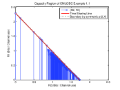
(a) before filter

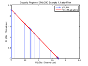
(b) after filter

Figure 1: Capacity region of Example 1, $\boldsymbol{\epsilon}^{(1)}=(0.05,0.24,0.71)$, $\boldsymbol{\epsilon}^{(2)}=(0.30,0.15,0.55)$.

Example 2.

Let $\boldsymbol{\epsilon}^{(1)}=(0.05,0.20,0.75)$, $\boldsymbol{\epsilon}^{(2)}=(0.30,0.15,0.55)$, the condition of case (ii) is satisfied. Numerical results are shown in Fig. 2 indicating that time sharing might be sufficient to exhaust the capacity region.

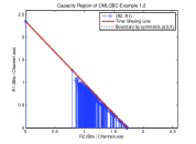
(a) before filter

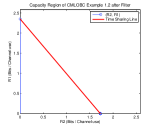
(b) after filter

Figure 2: Capacity region of Example 2, $\boldsymbol{\epsilon}^{(1)}=(0.05,0.20,0.75)$, $\boldsymbol{\epsilon}^{(2)}=(0.30,0.15,0.55)$.

Example 3.

Let $\boldsymbol{\epsilon}^{(1)}=(\rho_{1}^{2},\rho_{1},1-\rho_{1}-\rho_{1}^{2})$, $\boldsymbol{\epsilon}^{(2)}=(\rho_{2}^{2},\rho_{2},1-\rho_{2}-\rho_{2}^{2})$, where $0\leq\rho_{1}\leq\rho_{2}\leq(-1+\sqrt{5})/2$. This corresponds to Case (ii). Numerical results are shown in Fig. 3, for the particular case $\rho_{1}=0.1$, $\rho_{2}=0.3$ indicating that time sharing might be sufficient to exhaust the capacity region.

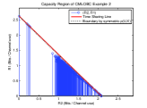
(a) before filter

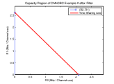
(b) after filter

Figure 3: Capacity Region of Example 3, $\boldsymbol{\epsilon}^{(1)}=(0.01,0.1,0.89)$, $\boldsymbol{\epsilon}^{(2)}=(0.09,0.3,0.61)$

Example 4.

let $q=2$, $m=3$, $l=2$, and define $\boldsymbol{\epsilon}^{(1)}=(0,\rho_{1},1-\rho_{1})$, $\boldsymbol{\epsilon}^{(2)}=(0,\rho_{2},1-\rho_{2})$. with $0\leq\rho_{1}\leq\rho_{2}\leq 1$, the condition of case (ii) is satisfied. Numerical results are shown in Fig. 4 for the particular case $\rho_{1}=0.1$, $\rho_{2}=0.3$ indicating that time sharing is suffice to exhaust the capacity region.

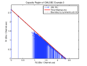
(a) before filter

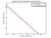
(b) after filter

Figure 4: Capacity Region of Example 4, $\boldsymbol{\epsilon}^{(1)}=(0,0.1,0.9)$, $\boldsymbol{\epsilon}^{(2)}=(0,0.3,0.7)$

IV-C A Conjecture on the Convexity of Capacity Region

Overall the analysis supports the conclusion that superposition coding on CMLOBCs has no benefit over simple time-sharing unless we are in Case (i). However, proving the conjecture in full generality seems to be difficult.

Conjecture.

For the degraded CMLOBCs described by (8), the capacity region is strictly concave ($\cap$) if and only if $\epsilon_{1}^{(1)}\epsilon_{2}^{(2)}>\epsilon_{1}^{(2)}\epsilon_{2}^{(1)}$.

IV-D A special example–The 7-ary erasure broadcast channel

Example 5.

Let $\boldsymbol{\epsilon}^{(1)}=(\rho_{1},0,1-\rho_{1})$, $\boldsymbol{\epsilon}^{(2)}=(\rho_{2},0,1-\rho_{2})$, where $0\leq\rho_{1}\leq\rho_{2}\leq 1$. Then the condition of Case (iii) is satisfied. Since (apart from unused output subspaces) there is now only one erasure symbol (the output subspace $\{\mathbf{0}\}$), the subchannels of the CMLOBC become $7$-ary erasure channels.

The capacity region of this broadcast channel, more generally of any CMLOBC with $\boldsymbol{\epsilon}^{(i)}=(\rho_{i},0,...,0,1-\rho_{i})$ for $i=1,2$, where $0\leq\rho_{1}\leq\rho_{2}\leq 1$, is determined by the next theorem. For the proof we need the following lemma.

Lemma 4.

Let $\mathsf{U}$, $\mathsf{X}$ and $\mathsf{Y}$ be random variables with alphabets $\mathfrak{U}$, $\mathfrak{X}$ and $\mathfrak{Y}$, respectively, forming a Markov chain $\mathsf{U\rightarrow\mathsf{X}\rightarrow\mathsf{Y}}$. Suppose that $\mathsf{X}\rightarrow\mathsf{Y}$ is described by

$$\bigl{(}p(Y_{j}|X_{i})\bigr{)}=\left(\begin{array}[]{ccc}\rho\mathbf{J}_{|\mathfrak{X}|\times 1}&|&(1-\rho)\mathbf{I}_{|\mathfrak{X}|\times|\mathfrak{X}|}\end{array}\right).$$ (11)

Then we have the relationships

$$I(\mathsf{U};\mathsf{Y})=(1-\rho)I(\mathsf{U};\mathsf{X}),$$ (12)

$$I(\mathsf{X};\mathsf{Y}|\mathsf{U})=(1-\rho)I(\mathsf{X};\mathsf{X}|U).$$ (13)

This follows from linearity of mutual information with respect to the decomposition (11) and $I(\mathsf{X};\mathsf{Y}|\mathsf{U})=I(\mathsf{X};\mathsf{Y})-I(\mathsf{U};\mathsf{Y})$.

Theorem 2.

Suppose that the two subchannels of a CMLOBC are described by

$$\mathbf{S}^{(i)}=\bigl{(}\rho_{i}\mathbf{J}_{|\mathfrak{X}|\times 1}\mid(1-\rho_{i})\mathbf{I}_{|\mathfrak{X}|\times|\mathfrak{X}|}\bigr{)},$$ (14)

where $\mathfrak{X}=\mathcal{P}(\mathbb{F}_{q}^{m},l)$ and $0\leq\rho_{1}\leq\rho_{2}\leq 1$. Then its capacity region is the set of all pairs of $(R_{1},R_{2})$ satisfying $R_{1},R_{2}\geq 0$ and

$$\frac{R_{1}}{(1-\rho_{1})\log|\mathfrak{X}|}+\frac{R_{2}}{(1-\rho_{2})\log|\mathfrak{X}|}\leq 1.$$ (15)

Proof.

See Appendix VII-E.∎

V Conclusion

In this paper, we have set up the framework of linear operator broadcast channels. We characterized degraded CMLOBCs by a set of inequalities for their associated probability vectors. Necessary and sufficient conditions for a CMLOBC being degraded were obtained. The work on CMLOBCs over $\operatorname{PG}(2,2)$ shows that time sharing schemes do not always exhaust the capacity region.

We conclude with some open problems arising from our work.

• In the case of more general CMLOBCs (i.e. less noisy, more capable), whose rate region is not exhausted by superposition coding, investigate whether other coding technologies (dirty paper coding, etc.) are suitable for approaching the boundary.

• How does the rate region of additive LOBCs or even more general LOBCs look like? The example of the binary symmetric broadcast channel suggests that in the generic case the nontrivial boundary curve $R_{2}=f(R_{1})$ is given by a strictly concave ($\cap$) function.

• Construct good (multishot) superposition subspace codes for degraded LOBCs in the case, where rate splitting is needed to approach the boundary of the rate region.

VI Acknowledgments

We wish to thank Prof. Ning Cai, Xidian University, Xi’an, China for helpful discussions and valuable suggestions for the proof of the outer bound of CMLOBCs. We are indebted to Kensuke Yasui, Hitachi Ltd., Japan for mailing us a Java script implementing the Arimoto-Blahut type algorithm.

VII Appendix

VII-A Proof of Lemma 1

Proof.

Suppose first that (ii) holds. Postmultiplying the equation $\boldsymbol{\epsilon}^{(1)}\boldsymbol{\Lambda}=\boldsymbol{\epsilon}^{(2)}$ by the matrix

$$\mathbf{L}=\left(\begin{array}[]{cccc}1&0&\cdots&0\\ 1&1&\cdots&0\\ \vdots&\vdots&\ddots&0\\ 1&1&\cdots&1\end{array}\right)$$ (16)

we obtain $\boldsymbol{\epsilon}^{(1)}\boldsymbol{\Lambda}\mathbf{L}=\boldsymbol{\epsilon}^{(2)}\mathbf{L}$. The matrix $\boldsymbol{\Delta}=\boldsymbol{\Lambda}\mathbf{L}=(\delta_{ij})$ is lower triangular with entries $\delta_{ij}\leq 1$. (This follows from $\delta_{ij}=\sum_{k=0}^{l}\lambda_{ik}l_{kj}=\sum_{k=j}^{l}\lambda_{ik}\leq\sum_{k=0}^{l}\lambda_{ik}=1$.) Hence we have

$$\sum_{i=j}^{l}\epsilon_{i}^{(2)} =(\boldsymbol{\epsilon}^{(2)}\mathbf{L})_{j}=(\boldsymbol{\epsilon}^{(1)}\boldsymbol{\Delta})_{j}$$

$$=\sum_{i=j}^{l}\epsilon_{i}^{(1)}\delta_{ij}\leq\sum_{i=j}^{l}\epsilon_{i}^{(1)}\,\,\,\,\,(0\leq j\leq l).$$

Then

$$\sum_{i=0}^{j}\epsilon_{i}^{(1)}=1-\sum_{i=j}^{l}\epsilon_{i}^{(1)}\leq 1-\sum_{i=j}^{l}\epsilon_{i}^{(2)}=\sum_{i=0}^{j}\epsilon_{i}^{(2)}$$

which implies (i).

Now suppose that (i) holds. First we consider the special case where $\boldsymbol{\epsilon}^{(1)}$ and $\boldsymbol{\epsilon}^{(2)}$ are related in the following way: There exist $0\leq i<j\leq l$ and a real number $0\leq\lambda\leq 1$ such that $\epsilon_{i}^{(2)}=\epsilon_{i}^{(1)}+\lambda\epsilon_{j}^{(1)}$, $\epsilon_{j}^{(2)}=(1-\lambda)\epsilon_{j}^{(1)}$ and $\epsilon_{k}^{(1)}=\epsilon_{k}^{(2)}$ for $k\in\{0,1,\dots,l\}\setminus\{i,j\}$. In this case we have $\boldsymbol{\epsilon}^{(1)}\boldsymbol{\Lambda}=\boldsymbol{\epsilon}^{(2)}$, where $\boldsymbol{\Lambda}$ differs from the identity matrix only in the submatrix corresponding to rows and columns No. $i$, $i+1$, …, $j$. The corresponding submatrix of $\boldsymbol{\Lambda}$ is

$$\begin{pmatrix}1\\ &\ddots\\ &&1\\ \lambda&&&1-\lambda\end{pmatrix},$$ (17)

so that $\boldsymbol{\Lambda}$ is clearly lower triangular and stochastic. In general, as is easily proved by induction, a new $\boldsymbol{\epsilon}^{(2)}$ can be updated from $\boldsymbol{\epsilon}^{(1)}$ and last $\boldsymbol{\epsilon}^{(2)}$ by a sequence of transformations of the above form (i.e., add $\lambda$ times the $j$-th component to the $i$-th component and subtract it from the $j$-th component for some $0\leq i<j\leq l$ and $0\leq\lambda\leq 1$). Since the set of lower triangular stochastic matrices is closed under matrix multiplication, the result follows. ∎

VII-B Proof of Lemma 2

Proof.

Working with the ordinary incidence matrices $\mathbf{D}_{ls}$, $\mathbf{D}_{st}$, $\mathbf{D}_{lt}$, the $(i,j)$-entry of $\mathbf{D}_{ls}\mathbf{D}_{st}$ is equal to the number of subspaces $V\in\mathcal{P}(\mathbb{F}_{q}^{m},s)$ satisfying $U_{i}\supseteq V\supseteq W_{j}$, where $U_{i}\in\mathcal{P}(\mathbb{F}_{q}^{m},l)$ and $W_{j}\in\mathcal{P}(\mathbb{F}_{q}^{m},t)$ denote the $i$-th resp. $j$-th subspace in the given ordering on $\mathcal{P}(\mathbb{F}_{q}^{m},l)$ resp. $\mathcal{P}(\mathbb{F}_{q}^{m},t)$. Thus

$$(\mathbf{D}_{ls}\mathbf{D}_{st})_{ij}=\begin{cases}\binom{l-t}{s-t}_{q}&\text{if $U_{i}\supseteq W_{j}$},\\ 0&\text{if $U_{i}\nsupseteq W_{j}$}.\end{cases}$$ (18)

This shows that $\mathbf{D}_{ls}\mathbf{D}_{st}=\binom{l-t}{s-t}_{q}\mathbf{D}_{lt}$ is a scalar multiple of $\mathbf{D}_{lt}$. Obviously we then also have $\mathbf{S}_{ls}\mathbf{S}_{st}=\lambda\mathbf{S}_{lt}$ for some scalar $\lambda$. Since $\mathbf{S}_{ls}\mathbf{S}_{st}$ as well as $\mathbf{S}_{lt}$ are stochastic, we must have $\lambda=1$, proving the lemma. ∎

VII-C Proof of Theorem 6

Proof.

Suppose first that Condition (6) is satisfied. In (5) we choose $\mathbf{T}_{ij}=\lambda_{ij}\mathbf{S}_{ij}$ with $\lambda_{ij}\in\mathbb{R}$ (where it is understood that $\mathbf{S}_{ij}=\mathbf{0}$ whenever $i<j$). Using Lemma 2 we obtain

$$\mathbf{S}^{(1)}\mathbf{T} =\bigl{(}\epsilon_{0}^{(1)}\mathbf{S}_{l0}\mid\epsilon_{1}^{(1)}\mathbf{S}_{l1}\mid\dots\mid\epsilon_{l}^{(1)}\mathbf{S}_{ll}\bigr{)}\times$$

$$\begin{pmatrix}\lambda_{00}\mathbf{S}_{00}&0&0&0\\ \lambda_{10}\mathbf{S}_{10}&\lambda_{11}\mathbf{S}_{11}&\cdots&0\\ \vdots&\vdots&\ddots&\vdots\\ \lambda_{l0}\mathbf{S}_{l0}&\lambda_{l1}\mathbf{S}_{l1}&\cdots&\lambda_{ll}\mathbf{S}_{ll}\end{pmatrix}$$ (19)

$$=\bigl{(}(\epsilon_{0}^{(1)}\lambda_{00}+\epsilon_{1}^{(1)}\lambda_{10}+\dots+\epsilon_{l}^{(1)}\lambda_{l0})\mathbf{S}_{l0},$$

$$\,\,\,\,\,\,\,\,(\epsilon_{1}^{(1)}\lambda_{11}+\epsilon_{1}^{(1)}\lambda_{21}\dots+\epsilon_{l}^{(1)}\lambda_{l1})\mathbf{S}_{l1},\dots,\epsilon_{l}^{(1)}\lambda_{ll}\mathbf{S}_{ll}\bigr{)}$$ (20)

By Lemma 1 we can further choose $\boldsymbol{\Lambda}=(\lambda_{ij})$ as a lower triangular stochastic matrix satisfying $\boldsymbol{\epsilon}^{(1)}\boldsymbol{\Lambda}=\boldsymbol{\epsilon}^{(2)}$. Then the resulting matrix $\mathbf{T}=(\lambda_{ij}\mathbf{S}_{ij})$ is stochastic and satisfies (5). Hence in this case the broadcast channel is degraded.

Conversely suppose the broadcast channel is degraded, so that (5) holds for some stochastic (block) matrix $\mathbf{T}=(\mathbf{T}_{ij})$. First we will show that we can assume (without loss of generality) that $\mathbf{T}_{ij}=0$ for $i<j$. (5) says

$$\sum_{i=0}^{l}\epsilon_{i}^{(1)}(\mathbf{S}_{li}\mathbf{T}_{ij})=\epsilon_{j}^{(2)}\mathbf{S}_{lj}\quad\text{for $0\leq j\leq l$}$$

If $\epsilon_{i}^{(1)}=0$ then we can replace each block $\mathbf{T}_{ij}$, $0\leq j\leq l$, by the corresponding all-zero matrix. Hence the assertion is true in this case. On the other hand, if $\epsilon_{i}^{(1)}>0$ then every positive entry in $\mathbf{S}_{li}\mathbf{T}_{ij}$ forces a positive entry of $\mathbf{S}_{lj}$ in the same position. Now suppose $\mathbf{T}_{ij}$ has a nonzero (i.e. positive) entry in a position indexed by some subspaces $V\in\mathcal{P}(\mathbb{F}_{q}^{m},i)$, $W\in\mathcal{P}(\mathbb{F}_{q}^{m},j)$. Then $\mathbf{S}_{li}\mathbf{T}_{ij}$ has a positive entry in each position indexed by the same subspace $W$ (as a column index) and any subspace $U\in\mathcal{P}(\mathbb{F}_{q}^{m},l)$ which contains $V$ (as a row index).

If $i<j$ then we can find a subspace $U\in\mathcal{P}(\mathbb{F}_{q}^{m},l)$ which contains $V$ but not $W$. This can be seen as follows: The space $\overline{W}=(W+V)/V$ is a nonzero subspace of $\mathbb{F}_{q}^{m}/V$. Hence there exists a subspace $\overline{U}$ of $\mathbb{F}_{q}^{m}/V$ of dimension $l-i<m-i$ which does not contain $\overline{W}$. Then the preimage $U$ of $\overline{U}$ in $\mathbb{F}_{q}^{m}$ has the required property. (The assumption $l<m$ is essential here!)

Since $U$ contains $V$ but not $W$, the matrix $\mathbf{S}_{li}\mathbf{T}_{ij}$ has an entry $>0$ in the position corresponding to $(U,W)$ and $\mathbf{S}_{lj}$ has a zero in this position. This contradiction shows that $\epsilon_{i}^{(1)}>0$ implies $\mathbf{T}_{ij}=0$ for $i<j$, so that from now on we can indeed assume $\mathbf{T}_{ij}=0$ for all $i<j$.

Now we postmultiply (5) by

$$\mathbf{L}=\begin{pmatrix}\mathbf{S}_{00}&0&\cdots&0\\ \mathbf{S}_{10}&\mathbf{S}_{11}&\cdots&0\\ \vdots&\vdots&\ddots&\vdots\\ \mathbf{S}_{l0}&\mathbf{S}_{l1}&\cdots&\mathbf{S}_{ll}\end{pmatrix}.$$ (21)

Using Lemma 2 on the left-hand side and setting $\boldsymbol{\Delta}=\mathbf{TL}=(\boldsymbol{\Delta}_{ij})$ on the right-hand side we obtain

$$\sum_{i=j}^{l}\epsilon_{i}^{(1)}\mathbf{S}_{li}\boldsymbol{\Delta}_{ij}=\left(\sum_{i=j}^{l}\epsilon_{i}^{(2)}\right)\mathbf{S}_{lj}\quad(0\leq j\leq l).$$ (22)

Applying these matrix equations to the all-one column vectors $\mathbf{j}$ of the appropriate dimensions gives, in view of $\mathbf{S}_{lj}\mathbf{j}=\mathbf{j}$ and $(\mathbf{S}_{li}\boldsymbol{\Delta}_{ij})\mathbf{j}=\mathbf{S}_{li}(\boldsymbol{\Delta}_{ij}\mathbf{j})\leq\mathbf{S}_{li}\mathbf{j}=\mathbf{j}$, the required inequalities $\sum_{i=j}^{l}\epsilon_{i}^{(2)}\leq\sum_{i=j}^{l}\epsilon_{i}^{(1)}$ ($0\leq j\leq l$), which completes the proof of the theorem. ∎

VII-D Proof of Lemma 3

Proof.

During the proof we write $\mathsf{Y}^{(i)}$, $i=1,2$, for the subchannel outputs (here $\mathsf{Y}^{(i)}$ corresponds to the probability vector $\epsilon^{(i)}$) and $\mathsf{Y}_{s}$, $s=0,1,2$, for the dimension $s$ component of $\mathsf{Y}^{(i)}$ (corresponding to the $s$-th block in the decomposition (8)), which is independent of $i$. We will use the (easily established) fact that mutual information is linear in the following sense:

$$I(\mathsf{X};\mathsf{Y}^{(1)}|\mathsf{U}) =\sum_{s=0}^{2}\epsilon_{s}^{(1)}I(\mathsf{X};\mathsf{Y}_{s}|\mathsf{U}),$$

$$I(\mathsf{U};\mathsf{Y}^{(2)}) =\sum_{s=0}^{2}\epsilon_{s}^{(2)}I(\mathsf{U};\mathsf{Y}_{s}),$$

which generalizes to arbitrary decompositions of the form (4).

Clearly $I(\mathsf{X};\mathsf{Y}_{0})=I(\mathsf{U};\mathsf{Y}_{0})=0$. The (symmetric) channels $\mathsf{X}\to\mathsf{Y}_{1}$, $\mathsf{X}\to\mathsf{Y}_{2}$, $\mathsf{U}\to\mathsf{Y}_{2}$ have channel matrices $\mathbf{S}_{21}$, $\mathbf{I}_{7\times 7}$, $\tfrac{\sigma}{6}\mathbf{J}_{7\times 7}+\left(1-\tfrac{7\sigma}{6}\right)\mathbf{I}_{7\times 7}$, respectively. The channel $\mathsf{U}\to\mathsf{Y}_{1}$ has channel matrix

$$\left(\tfrac{\sigma}{6}\mathbf{J}_{7\times 7}+\left(1-\tfrac{7\sigma}{6}\right)\mathbf{I}_{7\times 7}\right)\mathbf{S}_{21}=\tfrac{\sigma}{6}\mathbf{J}_{7\times 7}+\left(1-\tfrac{7\sigma}{6}\right)\mathbf{S}_{21}$$

The input distribution on $\mathfrak{U}$ (and hence the distribution on $\mathfrak{X}$ as well) is uniform, this gives

$$R_{2}(\sigma) =I(\mathsf{U};\mathsf{Y}^{(2)})$$

$$=\epsilon_{1}^{(2)}\left(-H\left(\tfrac{2\sigma}{3}\right)+\log\tfrac{7}{3}-\tfrac{2\sigma}{3}\log\tfrac{4}{3}\right)$$

$$\quad+\epsilon_{2}^{(2)}\left(-H(\sigma)+\log 7-\sigma\log 6\right),$$

$$R_{1}(\sigma) =I(\mathsf{X};\mathsf{Y}^{(1)}|\mathsf{U})$$

$$=\epsilon_{1}^{(1)}\left(H\left(\tfrac{2\sigma}{3}\right)+\tfrac{2\sigma}{3}\log\tfrac{4}{3}\right)$$

$$\quad+\epsilon_{2}^{(1)}\left(H(\sigma)+\sigma\log 6\right),$$

where $H(x)=-x\log x-(1-x)\log(1-x)$ denotes the binary entropy function. To simplify the expressions below, we will take $\log$ as the natural logarithm, for which $H^{\prime}(x)=\log\frac{1-x}{x}$, $H^{\prime\prime}(x)=-\frac{1}{x(1-x)}$. We have further

$$R_{2}^{\prime}(\sigma) =\epsilon_{1}^{(2)}\left(-\tfrac{2}{3}\log\tfrac{1-2\sigma/3}{2\sigma/3}-\tfrac{2}{3}\log\tfrac{4}{3}\right)$$

$$\quad+\epsilon_{2}^{(2)}\left(-\log\frac{1-\sigma}{\sigma}-\log 6\right)$$

$$=-\epsilon_{1}^{(2)}\tfrac{2}{3}\log\tfrac{2(1-2\sigma/3)}{\sigma}-\epsilon_{2}^{(2)}\log\tfrac{6(1-\sigma)}{\sigma},$$

$$R_{1}^{\prime}(\sigma) =\epsilon_{1}^{(1)}\tfrac{2}{3}\log\tfrac{2(1-2\sigma/3)}{\sigma}+\epsilon_{2}^{(1)}\log\tfrac{6(1-\sigma)}{\sigma}.$$

From this one verifies at once that $R_{1}^{\prime}(\sigma)>0$, $R_{2}^{\prime}(\sigma)<0$ for $0<\sigma<\frac{6}{7}$ (and $R_{1}^{\prime}(\frac{6}{7})=R_{2}^{\prime}(\frac{6}{7})=0$). Hence, by results from standard calculus, $f$ is well-defined and $f^{\prime}\bigl{(}R_{1}(\sigma)\bigr{)}=\frac{R_{2}^{\prime}(\sigma)}{R_{1}^{\prime}(\sigma)}<0$, so that $f$ is strictly decreasing. Moreover, since $R_{1}(0)=0$, $R_{2}(0)=\epsilon_{1}^{(2)}\log\tfrac{7}{3}+\epsilon_{2}^{(2)}\log 7=C_{2}$, $R_{1}(\tfrac{6}{7})=\epsilon_{1}^{(1)}\log\tfrac{7}{3}+\epsilon_{2}^{(1)}\log 7=C_{1}$, $R_{2}(\tfrac{6}{7})=0$, we have $f\colon[0,C_{1}]\to[0,C_{2}]$, $f(0)=C_{2}$, and $f(C_{1})=0$.

In order to decide whether $f$ is convex/concave/linear, we use the second derivative test from standard calculus. We have to determine the sign of

$$f^{\prime\prime}\bigl{(}R_{1}(\sigma)\bigr{)}=\frac{R_{2}^{\prime\prime}(\sigma)R_{1}^{\prime}(\sigma)-R_{1}^{\prime\prime}(\sigma)R_{2}^{\prime}(\sigma)}{R_{1}^{\prime}(\sigma)^{3}}$$

for $\sigma\in(0,\frac{6}{7})$, which is the same as the sign of

$$R_{2}^{\prime\prime}(\sigma)R_{1}^{\prime}(\sigma)-R_{1}^{\prime\prime}(\sigma)R_{2}^{\prime}(\sigma)=$$

$$=\frac{2(\epsilon_{1}^{(2)}\epsilon_{2}^{(1)}-\epsilon_{1}^{(1)}\epsilon_{2}^{(2)})}{\sigma(1-\sigma)(3-2\sigma)}\left((1-\sigma)\log\tfrac{6(1-\sigma)}{\sigma}\right.$$

$$\left.-\left(1-\tfrac{2\sigma}{3}\right)\log\tfrac{2(1-\tfrac{2\sigma}{3})}{\sigma}\right).$$ (23)

It may be verified that the right-hand factor

$$g(\sigma) =(1-\sigma)\log(1-\sigma)-\left(1-\tfrac{2\sigma}{3}\right)\log\left(1-\tfrac{2\sigma}{3}\right)$$

$$\quad+\tfrac{1}{3}\sigma\log\sigma+(1-\sigma)\log 6-\left(1-\tfrac{2\sigma}{3}\right)\log 2$$

satisfies $g(0)=g(\frac{6}{7})=0$ and

$$g^{\prime\prime}(\sigma)=-\frac{1}{\sigma(1-\sigma)(3-2\sigma)}<0\quad\text{for $0<\sigma<\tfrac{6}{7}$},$$

from which it follows that $g(\sigma)$ is positive in $(0,\frac{6}{7})$. Hence the sign of $f^{\prime\prime}$ in $(0,\frac{6}{7})$ is constant and equal to that of $\epsilon_{1}^{(2)}\epsilon_{2}^{(1)}-\epsilon_{1}^{(1)}\epsilon_{2}^{(2)}$. This concludes the proof.∎

VII-E Proof of Theorem 15

Proof.

It is clear from Lemma 13 that the capacities of the subchannels are $C_{i}=(1-\rho_{i})\log|\mathfrak{X}|$ ($i=1,2$). Further, for an arbitrary joint distribution $p(U,X)$ Lemma 13 gives

$$C_{2}I(\mathsf{X}; \mathsf{Y}_{1}|\mathsf{U})+C_{1}I(\mathsf{U};\mathsf{Y}_{2})$$

$$=(1-\rho_{2})\log|\mathfrak{X}|(1-\rho_{1})I(\mathsf{X};\mathsf{X}|\mathsf{U})$$

$$\quad+(1-\rho_{1})\log|\mathfrak{X}|(1-\rho_{2})I(\mathsf{U};\mathsf{X})$$

$$=\frac{C_{1}C_{2}}{\log|\mathfrak{X}|}\cdot I(\mathsf{X};\mathsf{X})$$

$$=\frac{C_{1}C_{2}}{\log|\mathfrak{X}|}\cdot H(\mathsf{X})\leq C_{1}C_{2},$$

which implies (15).∎

References

• [1] T. Ho, M. Medard, R. Koetter, D. Karger, M. Effros, J. Shi, and B. Leong, “A random linear network coding approach to multicast,” Information Theory, IEEE Transactions on, vol. 52, no. 10, pp. 4413 –4430, Oct. 2006.
• [2] R. Ahlswede, N. Cai, S.-Y. Li, and R. Yeung, “Network information flow,” Information Theory, IEEE Transactions on, vol. 46, no. 4, pp. 1204 –1216, Jul 2000.
• [3] R. Koetter and F. Kschischang, “Coding for errors and erasures in random network coding,” Information Theory, IEEE Transactions on, vol. 54, no. 8, pp. 3579 –3591, Aug. 2008.
• [4] D. Silva, F. Kschischang, and R. Kotter, “Communication over finite-field matrix channels,” Information Theory, IEEE Transactions on, vol. 56, no. 3, pp. 1296 –1305, Mar. 2010.
• [5] B. Uchôa-Filho and R. Nóbrega, “The capacity of random linear coding networks as subspace channels,” Arxiv preprint arXiv:1001.1021, 2010.
• [6] S. Yang, S. Ho, J. Meng, and E. hui Yang, “Optimality of subspace coding for linear operator channels over finite fields,” in Proc. IEEE Information Theory Workshop, 2010.
• [7] S. Yang, S. Ho, J. Meng, and E. Yang, “Linear operator channels over finite fields,” Arxiv preprint arXiv:1002.2293, 2010.
• [8] M. Jafari, S. Mohajer, C. Fragouli, and S. Diggavi, “On the capacity of non-coherent network coding,” in Proceedings of the 2009 IEEE international conference on Symposium on Information Theory-Volume 1.   Institute of Electrical and Electronics Engineers Inc., The, 2009, pp. 273–277.
• [9] T. Cover and J. Thomas, “Elements of information theory,” Wiley Series In Telecommunications, p. 542, 1991.
• [10] E. van der Meulen, “A survey of multi-way channels in information theory: 1961-1976,” Information Theory, IEEE Transactions on, vol. 23, no. 1, pp. 1 – 37, Jan. 1977.
• [11] T. Cover, “Comments on broadcast channels,” Information Theory, IEEE Transactions on, vol. 44, no. 6, pp. 2524 –2530, Oct 1998.
• [12] E. Calvo, D. Palomar, J. Fonollosa, and J. Vidal, “The computation of the capacity region of the discrete degraded bc is a nonconvex DC problem,” in Information Theory, 2008. ISIT 2008. IEEE International Symposium on, 2008, pp. 1721 –1725.
• [13] K. Yasui and T. Matsushima, “Toward computing the capacity region of degraded broadcast channel,” in Information Theory Proceedings (ISIT), 2010 IEEE International Symposium on, 2010, pp. 570 –574.
• [14] S. Arimoto, “An algorithm for computing the capacity of arbitrary discrete memoryless channels,” vol. 18, no. 1, pp. 14–20, Jan. 1972.
• [15] R. E. Blahut, “Computation of channel capacity and rate-distortion functions,” vol. 18, no. 4, pp. 460–473, Jul. 1972.
• [16] A. Dana and B. Hassibi, “The capacity region of multiple input erasure broadcast channels,” in Information Theory, 2005. ISIT 2005. Proceedings. International Symposium on, 4-9 2005, pp. 2315 –2319.
• [17] Y. Pang and T. Honold, “M-files to compute the capacity region of degraded CMLOBCs,” 2010. [Online]. Available: http://rapidshare.com/files/439653424/DegradedCMLOBCs.zip