Directed transport driven by the transverse wall vibration

Abstract

Directed transport of overdamped Brownian particles in an asymmetrically periodic tube is investigated in the presence of the tube wall vibration. From the Brownian dynamics simulations we can find that the perpendicular wall vibration can induce a net current in the longitudinal direction when the tube is asymmetric. The direction of the current at low frequency is opposite to that at high frequency. One can change the direction of the current by suitably tailoring the frequency of the wall vibration.

I Introduction

Stochastic transport on periodic asymmetric substrates far from equilibrium has raised widespread interest in the recent literature a1 . In these spatially periodic structures, directed motion of particles can induced by zero-mean nonequilibrium fluctuations and noise. These come from the desire to understand molecular motorsa2 , nanoscale frictiona3 , surface smoothinga4 , coupled Josephson junctionsa5 , optical ratchets and directed motion of laser-cooled atomsa6 , and mass separation and trapping schemes at the microscalea7 . The fundamental condition for directed transport to occur is that either the spatial reflection symmetry of the system is broken or fluctuations are statistically asymmetric. Several models have been proposed to explain this transport mechanism under various nonequlibrium situations. Typical examples are rocking ratchets a8 , flashing ratchetsa9 , diffusion ratchetsa10 , correlation ratchetsa11 .

Most studies have revolved around the energy barrier. The nature of the barrier depends on which thermodynamic potential varies when passing from one well to the other, and its presence plays an important role in the dynamics of the system. However, in many transport phenomenaa12 , such as those taking place in micro- and nano-pores, zeolites, biological cells, ion channels, nanoporous materials and microfluidic devices etched with grooves and chambers, Brownian particles, instead of diffusing freely in the host liquid phase, undergo a constrained motion. In these cases the entropic barriers may appear when coarsening the description of a complex system in order to simplify its dynamics. Reguera and coworkersa13 used the mesoscopic nonequilibrium thermodynamics theory to derive the general kinetic equation of the motor system and analyzed in detail the case of diffusion in a domain of irregular geometry in which the presence of the boundaries induces an entropy barrier when approaching the dynamics by a coarsening of the description. In their recent work a14 they studied the current and the diffusion of a Brownian particle moving in a symmetric channel with a biased external force. In our previous worka15 , we studied the transport of overdamped particles in a three dimensional tube in the presence of unbiased external forces and the motion of particles can indeed be rectified, with a sign that depends on the details of the wall profile. In the present work, we study the directed transport of overdamped Brownian particles moving in asymmetric tube in the presence of the tube wall vibration. We emphasized on finding whether the transverse wall vibration can induce a longitudinal net current and how the parameters of the system affect the transport.

II Model and Methods

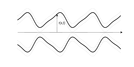
Figure 1: Schematic diagram of a tube with periodicity $L$. The vibrating wall is described by its time dependent half width $r(x,t)=a[\sin(\frac{2\pi x}{L})+\frac{\Delta}{4}\sin(\frac{4\pi x}{L})]+b+b_{0}\sin(\omega t)$. $\Delta$ is the asymmetric parameter of the tube shape and $\Delta=-1.0$ in the diagram. The solid line describes the original shape of the tube and the dotted line shows its vibrating shape.

In this study, we study the transport of the particles in an asymmetrically periodic tube driven by the tube wall vibration [Fig. 1]. Since most of the molecular transport occurs in the overdamped regime, we can safely neglect inertial effects. The overdamped dynamics can be described by the following Langevin equations written in a dimensionless form a14 ; a15 ,

$$\eta\frac{dx}{dt}=\sqrt{\eta k_{B}T}\xi_{x}(t),$$ (1)

$$\eta\frac{dy}{dt}=\sqrt{\eta k_{B}T}\xi_{y}(t),$$ (2)

where $x$, $y$, are the two-dimensional (2D) coordinates, $\eta$ is the friction coefficient of the particles, $k_{B}$ is the Boltzmann constant, $T$ is the absolute temperature and $\xi_{x,y}(t)$ is the Gaussian white noise with zero mean and correlation function: $<\xi_{i}(t)\xi_{j}(t^{{}^{\prime}})>=2\delta_{i,j}\delta(t-t^{{}^{\prime}})$ for $i,j=x,y$. $<...>$ denotes an ensemble average over the distribution of noise. $\delta(t)$ is the Dirac delta function. Imposing reflecting boundary conditions in the transverse direction ensures the confinement of the dynamics within the tube, while periodic boundary conditions are enforced along the longitudinal direction for the reasons noted above. The vibrating wall is described by its time dependent half width

$$r(x)=a[\sin(\frac{2\pi x}{L})+\frac{\Delta}{4}\sin(\frac{4\pi x}{L})]+b+b_{0}\sin(\omega t),$$ (3)

where $a$ is the parameter that controls the slope of the tube and $\Delta$ is the asymmetric parameter of the tube shape. $b$ is the parameter that determines the half width at the bottleneck. $b_{0}$ and $\omega$ are the amplitude and frequency of the vibration, respectively.

In this case, no general valid analytical expressions are possible. However, the study of these transport phenomena is in many respects equivalent to an investigation of geometrically constrained Brownian dynamicsb1 . The behavior of the quantities of interest have been corroborated by Brownian dynamic simulations performed by integration of the Langevin equation using the standard stochastic Euler algorithm. The average particle velocity in the $x$-direction has been derived from an ensemble average of about $3\times 10^{4}$ trajectories according to the following expression. From Eq. (1-2) and the standard stochastic Euler algorithm, the single integration steps read b1 :

$$x_{new}=x_{old}+\sqrt{2k_{B}T\Delta t}R_{1},$$ (4)

$$y_{new}=y_{old}+\sqrt{2k_{B}T\Delta t}R_{2},$$ (5)

if $|y_{new}|<|r(x_{new})|$, the modification positions of $x,y$-coordinate are

$$x_{old}=x_{new},\indent y_{old}=y_{new},$$ (6)

if $|y_{new}|\geq|r(x_{new})|$, the particles will meet the wall. In this case, we use a simple way to simulate the movement of particles near the wall: When the particles meet the wall, it will return to its previous position and the time step is incremented, namely,

$$x_{old}=x_{old},\indent y_{old}=y_{old},$$ (7)

where $x_{old}$, $y_{old}$ are the original positions and $x_{new}$, $y_{new}$ are the new positions. $R_{1}$, $R_{2}$ are two Gaussian distributed random numbers with unit variance. $\Delta t$ is the integration step time. The average particle velocity along the $x$-direction,

$$\nu=\langle\dot{x}\rangle=\lim_{t\rightarrow\infty}\frac{\langle x(t)\rangle}{t}.$$ (8)

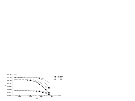
Figure 2: Dependence of the mean velocity $v$ on time step $\Delta t$. (a)for different values of temperature at $\Delta=-1.0$, $\omega=11.0$, $a=0.5$, $b=0.9$, $b_{0}=0.3$, and $L=1.0$. The full symbols depict the present algorithm and the empty symbols indicate the strict reflection algorithm. (b) for different parameters at $\Delta=-1.0$, $a=0.5$, $b_{0}=0.3$, and $L=1.0$.

In order to check the validity of the present Brwonian dynamics algorithm, it is necessary to compare the present results with a real reflecting boundary condition on the wall. From Fig. 2(a), we can find that the results from the present algorithm well agree with that from the strict reflection algorithm for very small time step. Moreover, the present algorithm takes much less CPU time than the strict reflection one. We have also checked the convergence of the algorithm in a large range of the system parameters. From Fig. 2 we can see that the algorithm is convergent and the numerical results will not depend on the time step for very small time step. Therefore, our algorithm will give well approximate results with respect to the strict reflection algorithm. In order to provide the requested accuracy of the system dynamics time step was chosen to be smaller than $10^{-4}$.

We must point that the extension of our scheme to three-dimension with rotational symmetry along the transport axis is possible as well. This will consume more computation time, but the over results remain qualitatively robust.

III Numerical results and discussion

Our emphasis is on finding the asymptotic mean velocity which is defined as the average of the velocity over the time and thermal fluctuations. In order to obtain the mean velocity, we carried out extensive numerical simulations based on Eq. (4-8). For simplicity we set $\eta=1$ and $k_{B}=1$ throughout the work.

Figure 3: The mean velocity $v$ as a function of vibrating frequency $\omega$ for different values of asymmetric parameter $\Delta=-1.0$, $0.0$, and $1.0$ at $T=0.05$, $a=0.5$, $b=0.9$, $b_{0}=0.3$, and $L=1.0$. $\omega_{L}$ is the frequency for the left peak, $\omega_{C}$ is the cross-over frequency and $\omega_{R}$ denotes the frequency for the right valley.

.

Figure 3 shows the mean velocity $v$ as a function of the vibrating frequency $\omega$. From the Fig. 3, we can see that for low frequencies the current is positive for $\Delta<0$, zero at $\Delta=0$, and negative for $\Delta>0$. The phenomenon will be opposite to that for high frequencies. It is obvious that the symmetry between the curve $\Delta=1.0$ and $\Delta=-1.0$ is due to the symmetry of geometry. Now we will focus on the case of $\Delta=-1.0$, namely, the right side is steeper than the left one. In the adiabatic limit $\omega\rightarrow 0$, the vibration can be expressed by two opposite static driving $-b_{0}$ and $b_{0}$ and the nonequilibrium system reduces to the system with two equilibrium states, namely, $v=\frac{1}{2}[v(-b_{0})+v(b_{0})]=0$. For low frequencies, the particles get enough time to reach the whole area and the wall will act on the particles. In this case, the probability of the particles acting on the slanted wall (the left wall) is larger than that on the steeper wall (the right wall), resulting in a positive current. On increasing the frequency $\omega$, due to high frequency, the Brownian particles do not get enough time to reach the slanted wall (The area of the slanted side is larger than that of the steep one). Therefore, the probability of the particles acting on the slanted wall is smaller than that on the steep wall, yielding a negative current. When the vibration changes very fast $\omega\rightarrow\infty$, the particles can not experience the changes of the wall and the system reduces to a equilibrium system, so the current goes to zero. Therefore, the direction of the current can be controlled by changing the vibrating frequencies.

In order to give more detail insight into the characteristic frequencies $\omega_{L}$, $\omega_{C}$, and $\omega_{R}$, we corroborate the numerical estimates of the frequencies for a larger range of parameter values. The numerical estimates are shown in Fig 4. We find that the characteristic frequencies increase with temperature $T$ and the length of the period $L$ and decrease with the vibrating amplitude $b_{0}$. The estimated exponential relations are also shown in the figure. From the figure we can obtain the approximate scaling results for $\omega_{L}\propto T^{0.64}b_{0}^{-1.57}L^{-0.95}$, $\omega_{C}\propto T^{0.71}b_{0}^{-1.31}L^{-1.32}$, and $\omega_{R}\propto T^{0.72}b_{0}^{-1.07}L^{-1.41}$. It is obvious that these characteristic frequencies will shift to large values for high temperature and to small values for large amplitude of the vibration.

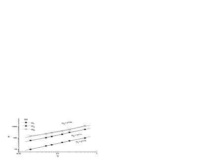
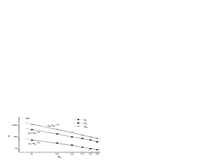
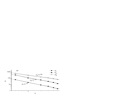
Figure 4: Dependence of characteristic frequencies $\omega_{L}$, $\omega_{C}$, and $\omega_{R}$ on the different parameters. (a)On temperature $T$ at $a=0.5$, $b=0.9$, $b_{0}=0.3$, $\Delta=-1.0$, and $L=1.0$. (b)On the vibrating amplitude $b_{0}$ at $T=0.05$, $a=0.5$, $b=0.9$,$\Delta=-1.0$, and $L=1.0$. (c)On the period $L$ at $T=0.05$, $a=0.5$, $b=0.9$,$b_{0}=0.3$, and $\Delta=-1.0$. The solid lines are the fitting lines.

Figure 5: (a)The mean velocity $v$ as a function of temperature $T$ at $a=0.5$, $b=0.9$, $b_{0}=0.3$, $\Delta=-1.0$, $\omega=10.0$, and $L=1.0$. $T_{C}$ is the optimized value of temperature for the peak. (b)Dependence of $T_{C}$ on the driving frequency $\omega$ at $a=0.5$, $b=0.9$, $b_{0}=0.3$, and $\Delta=-1.0$. (c)Dependence of $T_{C}$ on the driving amplitude $b_{0}$ at $a=0.5$, $b=0.9$, $\omega=10.0$, and $\Delta=-1.0$. The solid lines are the fitting lines.

In order to investigate how the temperature affects the transport, we also show the mean velocity as a function of temperature in Fig. 5(a) at $\Delta=-1.0$ and $\omega=10.0$. The diffusion from the temperature has two roles: jumping from one cell to another in longitudinal direction and making the particles acting on the wall in transverse direction. When $T\rightarrow 0$, the particles cannot reach the wall and the effect of wall disappears and there is no current. When $T\rightarrow\infty$, the effect of the wall vibration disappears and the current goes to zero, also. Therefore, there is an optimized value of $T$ at which the mean velocity $v$ takes its maximum value, which indicates that the thermal noise may facilitate the particles transport. In order to give a feeling of the generality of the optimized value of temperature, we also study the dependence of $T_{C}$ on the vibrating frequency and amplitude. From Fig. 5 (b) and (c), we can obtain the approximate scaling results for the optimized temperature $T_{C}\propto b_{0}^{0}\omega^{0.86}$. The value of the optimized temperature will become larger for high driving frequency. Remarkably, the optimized temperature is independent of the driving amplitude.

Figure 6: (a)The mean velocity $v$ as a function of parameter $b$ at $a=0.5$, $b_{0}=0.3$, $\Delta=-1.0$, $\omega=10.0$, $T=0.05$, and $L=1.0$. $b_{C}$ denotes the optimized value of $b$ for the peak. (b)Dependence of $b_{C}$ on temperature $T$ at $a=0.5$, $b_{0}=0.3$, $\Delta=-1.0$, $\omega=10.0$, and $L=1.0$. (b)Dependence of $b_{C}$ on the driving frequency $\omega$ at $a=0.5$, $b_{0}=0.3$, $\Delta=-1.0$, $T=0.05$, and $L=1.0$. The solid lines are the fitting lines.

Figure 6 (a) shows the mean velocity $v$ as a function of the controlling parameter $b$. The parameter $b$ determines the radius at the bottleneck. The tube may be close for too small values of $b$. If the radius at the bottleneck is small few particles can pass from one cell to another, so the mean velocity is small. When the bottleneck has infinite radius ($b\rightarrow\infty$), the tube reduces to a straight one and the effect of tube shape disappears, so the current goes to zero. Therefore, there exists a value of $b_{C}$ at which the mean velocity takes its maximum. We also study how the temperature $T$ and the vibrating frequency $\omega$ affect the optimized value $b_{C}$. From the numerical simulations, we also find the approximate scaling results for $b_{C}\propto T^{-0.16}\omega^{0.11}$. It is found that $b_{C}$ decreases with temperature $T$ and increases wit the vibrating frequency $\omega$.

Figure 7: The mean velocity $v$ as a function of vibrating amplitude $b_{0}$ at $a=0.5$,$b=0.9$, $\Delta=-1.0$, $\omega=10.0$, $T=0.05$, and $L=1.0$.

Figure 7 gives the mean velocity $v$ as a function of the vibrating amplitude $b_{0}$. When $b_{0}\rightarrow 0$, the particles can not experience the wall vibrating, so the current goes to zero. On increasing the vibrating amplitude $b_{0}$, the mean velocity increases. However, for large values of $b_{0}$, the tube may be close at some time, then the current decreases. We must point out that for very large value of $b_{0}$, the profiles of tube wall may be exchanged, this is not true for a real system.

IV Concluding Remarks

In this paper, we study the transport of overdamped Brownian particles moving in an asymmetrically periodic tube with the wall vibration. From the numerical simulation we can find that the transverse wall vibration can induce a net longitudinal current in an asymmetrically periodic tube. We can have current reversals by changing the sign of $\Delta$, the asymmetry of the tube. The sign of mean velocity for low frequencies is opposite to that for high frequencies. Therefore, we can change the direction of the current by suitably tailoring the vibrating frequency. Thus, varying the asymmetry of the tube and the vibrating frequency are the two ways of inducing current reversals. These peculiar reversals are due to different strength and asymmetry of relaxation processes. The symmetry of relaxation processes changes with the system parameters, so the current may changes its direction when the parameters are changed. In addition, there exists an optimized value of temperature at which the mean velocity takes its maximum value, which indicates that the thermal noise may facilitate the particles transport.

Clearly, the model is too simple to provide a realistic description of real systems, however, the results we have presented have a wide application in may processes, such as diffusion of ions and macromolecular solutes through the channels in biological membranesc1 , transport in zeolitesc2 and nanostructures of complex geometry c3 , controlled drug releasec4 , and diffusion in man-made periodic porous materialsa12 . It is very important to understand the novel properties of these confined geometries, zeolites, biological channels, nanoporous materials, and microfluidic devices, as well as the transport behavior of species in these systems.

The author is very grateful to the two anonymous reviewers for the valuable comments and suggestions. This work was supported in part by National Natural Science Foundation of China with Grant No. 30600122 and GuangDong Provincial Natural Science Foundation with Grant No. 06025073.

References

- (1) P. Reimann, Phys. Rep.361, 57 (2002); P. Hanggi and F. Marchesoni, Rev. Mod. Phys. 81, 387 (2009).
- (2) R. D. Astumian, Science 176, 917 (1997); J. Maddox, Nature (London) 368 287(1994).
- (3) C. Daly, J. Krim, Phys. Rev. Lett. 76, 803(1996) 803; J. Krim, D.H. Solina, R. Chiarello, Phys. Rev. Lett. 66 ,181(1991); L. Daikhin, M. Urbakh, Phys. Rev. E 49,1424(1994).
- (4) I. Derenyi, C. Lee, and A. L. Barabasi, Phys. Rev. Lett. 80, 1473(1998).
- (5) I. Zapata, R. Bartussek, F. Sols, P. Hanggi, Phys. Rev. Lett. 77, 2292 (1996).
- (6) C. Mennerat-Robilliard, D. Lucas, S. Guibal, J. Tabosa, C. Jurczak, J.-Y. Courtois, G. Grynberg, Phys. Rev. Lett. 82, 851(1999); L.P. Faucheux, L.S. Bourdieu, P.D. Kaplan, A.J. Libchaber, Phys. Rev. Lett. 74,1504 (1995).
- (7) T. A. J. Duke, R. H. Austin, Phys. Rev. Lett. 80, 1552 (1998); L. Gorre-Talini, J.P. Spatz, P. Silberzan, Chaos 8, 650 (1998); I. Derenyi, R.D. Astumian, Phys. Rev. E 58, 7781 (1998); D. Ertas, Phys. Rev. Lett. 80, 1548 (1998).
- (8) R. D. Astumian and M. Bier, Phys. Rev. Lett. 72, 1766 (1994); M. O. Magnasco, Phys. Rev. Lett. 71, 1477 (1993).
- (9) P. Reimann, Phys. Rep. 290, 149(1997); J. D. Bao and Y. Z. Zhuo, Phys. Lett. A 239, 228 (1998); B. Q. Ai, L. Q. Wang, and L. G. Liu, Chaos, Solitons Fractals 34, 1265 (2007).
- (10) P. Reimann, R. Bartussek, R. Haussler, and P. Hanggi, Phys. Lett. A 215, 26 (1994).
- (11) C. R. Doering, W. Horsthemke, and J. Riordan, Phys. Rev. Lett. 72, 2984 (1994).
- (12) T. Chou and D. Lohse, Phys. Rev. Lett. 82, 3552 (1999); L. Liu, P. Li, and S.A. Asher, Nature 397, 141 (1999); S. Matthias and F. M uller, Nature 424, 53 (2003).
- (13) D. Reguera and J. M. Rubi, Phys. Rev. E 64, 061106 (2001).
- (14) D. Reguera, G. Schmid, P. S. Burada, J. M. Rubi, P. Reimann, and P. Hanggi, Phys. Rev. Lett. 96, 130603 (2006); P. S. Burada, G. Schmid, P. Talkner, P. Hanggi, D. Reguera, and J. M. Rubi, BioSystems 93, 16 (2008).
- (15) B. Q. Ai and L. G. Liu, Phys. Rev. E 74, 051114 (2006); B. Q. Ai, Phys. Rev. E 80, 011113 (2009); B. Q. Ai and L. G. Liu, J. Chem. Phys. 126, 204706 (2007).
- (16) P. S. Burada, P. Hanggi, F. Marchesoni, G. Schmid, and P. Talkner,ChemPhysChem 10, 45 (2009); P. S. Burada, G. Schmid, D. Reguera, J. M. Rubi, and P. Hanggi, Phys. Rev. E 75, 051111 (2007); A. M. Berezhkovskii, M. A. Pustovoit, and S. M. Bezrukov, J. Chem. Phys. 126, 134706 (2007).
- (17) B. Hille, Ion Channels in Excitable Membranes (Sinauer Associates, Sunderland, MA, 2001).
- (18) J. Karger and D. M. Ruthven, Diffusion in Zeolites and Other Microporous Solids (Wiley, New York, 1992).
- (19) N. F. Sheppard, D. J. Mears, and S. W. Straks, J. Controlled Release 42, 15 (1996).
- (20) J. T. Santini, Jr., M. J. Cima, and R. Langer, Nature (London) 397, 335 (1999); R. A. Siegel, J. Controlled Release 69, 109 (2000).