The complex universe: recent observations and theoretical challenges

Abstract

The large scale distribution of galaxies in the universe displays a complex pattern of clusters, super-clusters, filaments and voids with sizes limited only by the boundaries of the available samples. A quantitative statistical characterization of these structures shows that galaxy distribution is inhomogeneous in these samples, being characterized by large-amplitude fluctuations of large spatial extension. Over a large range of scales, both the average conditional density and its variance show a nontrivial scaling behavior: at small scales, $r<20$ Mpc/h, the average (conditional) density scales as $r^{-1}$. At larger scales, the density depends only weakly (logarithmically) on the system size and density fluctuations follow the Gumbel distribution of extreme value statistics. These complex behaviors are different from what is expected in a homogeneous distribution with Gaussian fluctuations. The observed density inhomogeneities pose a fundamental challenge to the standard picture of cosmology but it also represent an important opportunity which points to new directions with respect to many cosmological puzzles. Indeed, the fact that matter distribution is not uniform, in the limited range of scales sampled by observations, rises the question of understanding how inhomogeneities affect the large-scale dynamics of the universe. We discuss several attempts which try to model inhomogeneities in cosmology, considering their effects with respect to the role and abundance of dark energy and dark matter.

1 Introduction

Cosmological observations are usually interpreted within a theoretical framework based on the simplest conceivable class of solutions of Einstein’s law of gravitation. Namely, by using the assumptions that the universe is homogeneous and isotropic, one is able to work out, from the Einstein’s field equations, the dynamics of space-time. The Friedmann-Robertson-Walker (FRW) geometry is derived under these two assumptions and it describes the geometry of the universe in terms of a single function, the scale factor, which obeys to the Friedmann equations [1]. In this situation, the matter density is constant in a spatial hyper-surface. On the top of the constant matter density one can consider a statistically homogeneous and isotropic small-amplitude fluctuations field. These fluctuations furnish the seeds of gravitational clustering which will eventually give rise to the structures we observe in the present universe. Evolution of fluctuations is not considered to have a sensible effect on the evolution of the space-time which is instead driven by the uniform mean field.

While the simplicity of this scenario has its own appeal, in the standard model of cosmology one has to conjecture the existence of two fundamental constituents, if observational constraints are met, that both have yet unknown origin: first, a dominant repulsive component is thought to exist that can be modeled, for instance, by a positive cosmological constant. The physical nature of this component, named Dark Energy, is yet unknown and its abundance cannot be inferred from a-priori principles, whilst it is widely believed that dark energy is the biggest puzzle in standard cosmology today; e.g., the value of the cosmological constant in cosmology seems absurdly small in the context of quantum physics [2].

There is, secondly, a non-baryonic component that should considerably exceed the contribution by luminous and dark baryons and massive neutrinos. This component, named non-baryonic Dark Matter, is thought to be provided by exotic forms of matter, not yet detected in laboratory experiments. The main peculiar property of this matter component is that of weakly interacting with radiation in order to met the observational constraints given by observations [3]. According to the concordance model of standard cosmology, the contribution of the former converges to about 3/4 and that for the latter to about 1/4 of the total source of the standard cosmological equations (Friedmann equations), while up to a few percent has to be attributed to what is instead directly measurable by observations, namely ordinary baryonic matter, radiation and neutrinos.

If the underlying cosmological model is not a perturbation of an exact flat FRW solution, the conventional data analysis and their interpretation is not necessarily valid and thus the estimations of Dark Matter and Dark Energy can be questionable. The breaking of the FRW solution can be caused, for instance, by strong inhomogeneities of large spatial extension in the matter distribution. If this were the case, the theoretical problem would then concern of whether inhomogeneous properties of the Universe can be described by the strong FRW idealization and/or in which limit this would be so.

The question of whether observations of galaxy structures satisfy, on some scales, the assumptions used to derive the FRW metric is thus central. Surprisingly enough, studies of the large scale distribution of matter in the universe, as sampled by galaxy structures, seem not to be trivially compatible with such a theoretical scenario. Indeed, more and more structures on larger and larger scales have been discovered in the course of the last two decades with the advent of the three dimensional maps of the large scale universe. There structures were unexpected both because two-dimensional (angular) surveys were rather uniform and because theoretical models were unable to predict the existence of them. In many cases it was concluded that the particular three-dimensional survey under consideration had picked up a particularly “rare” fluctuation: this was in respect to the Gaussian distribution of fluctuations predicted by theoretical models. The statistical characterization of these structures, determining the range of correlations and the amplitudes and sizes of inhomogeneities, has thus posed a fundamental challenge to the standard picture of cosmology. The key-problem would be then to include these large fluctuations in the cosmological dynamics in a coherent way.

As long as structures are limited to small sizes, and fluctuations have low amplitude, one can just treat fluctuations as small-amplitude perturbations to the leading order FRW approximation. However if structures have “large enough” sizes and “high enough” amplitudes, a perturbation approach may loose its validity and a more general treatment of inhomogeneities needs to be developed. From the theoretical point of view, it is then necessary to understand how to treat inhomogeneities in the framework of General Relativity. In this context the first issue is whether inhomogeneities can be described by the FRW idealization at least on average, by postulating that on large enough scales uniformity is eventually reached. In other words, the key-question is: does an inhomogeneous model of the Universe at relatively small scales and, uniform at large scales, evolves on average like a homogeneous solution of Einstein’s law of gravitation ? Currently there is a wide discussion in the literature on this issue because, in the framework of averaged cosmological equations that has been provided by Buchert [4], it was found that a potential way to explain Dark Energy (and possibly also Dark Matter) can be, partially or fully, given by an effect of structure formation in an inhomogeneous cosmology. Inhomogeneities may mimic the effect of Dark Energy [5].

Thus, while observations of galaxy structures have given an impulse to the search for more general solution of Einstein’s equations than the Friedmann one, it is now under an intense investigation whether such a more general framework may provide a different explanation to the various effects that, within the standard FRW model, have been interpreted as Dark Energy and Dark Matter.

In these proceedings we first review in Sect.2 the situation with respect to galaxy structures: their observations and the analysis of their statistical properties. We then discuss in Sect.3 the implications of the results on galaxy distribution with respect to the standard theoretical assumptions of the FRW model. This allows us to properly frame the problem of inhomogeneities from the point of view of theoretical modeling. We then draw, in Sect.4, our main conclusions.

2 Size and amplitude of galaxy structures

In one of his seminal papers, Gerard de Vaucouleurs [6] put into an historical perspective the problem of galaxy large scale structures and the question about the scale where galaxy distribution turns to uniformity (where by uniformity it is meant the absence of structures of large amplitude or, in other words, of the absence voids — see below). He pointed out that observations have firstly found that galaxies are not randomly distributed. Then, that in the fifties the same property was assigned to cluster centers. Finally that at the end of the sixties the discovery of super-clusters has still enlarged the scale of structures in the universe thus pushing to larger and larger scales the scale where the approach to uniformity occurs. In the last twenty years many observations have been dedicated to the study of the three-dimensional large-scale distributions of galaxies [7, 8, 9, 10, 11]. In particular during the last decade two ambitious observational programs have measured the redshift of more than one million objects [12, 13]. All these surveys have detected larger and larger structures, thus finding that galaxies are organized in a complex network of clusters, super-clusters, filaments and voids.

For instance the famous “slice of the Universe”, that represented the first set of observations done for the CfA Redshift Survey in 1985 [14], mapped spectroscopic observations of about 1100 galaxies in a strip on the sky 6 degrees wide and about 130 degrees long. This initial map was quite surprising, showing that the distribution of galaxies in space was anything but random, with galaxies actually appearing to be distributed on surfaces, almost bubble like, surrounding large empty regions, or “voids.”. The structure running all the way across the survey between 50 and 100 Mpc/h was called the “Great Wall” and at the time of the discovery was the largest single structure detected in any redshift survey. Its dimensions, limited only by the sample size, are about $200\times 80\times 10$ Mpc/h, a sort of like a giant quilt of galaxies across the sky [15]. More and more galaxy large scale structures were identified in the other redshift surveys such as the Perseus-Pisces super-cluster [9] which is one of two dominant concentrations of galaxies in the nearby universe. This long chain of galaxies lies next to the the so-called Taurus void, which is a large circular void bounded by walls of galaxies on either side of it. The void has a diameter of about 30 Mpc/h. Few years ago, in the larger sample provided by the Sloan Digital Sky Survey (SDSS) [13], it has been discovered the Sloan Great Wall [16], which is a giant wall of galaxies and which is the largest known structure in the Universe, being nearly three times longer than the Great Wall.

2.1 A characteristic scale for galaxy clustering ?

Despite the fact that large scale galaxy structures, of size of the order of several hundreds of Mpc/h, have been observed to be the typical feature of the distribution of visible matter in the local universe, the statistical analysis measuring their properties has identified a characteristic scale which has only slightly changed since its discovery fourthy years ago in angular catalogs. Surprisingly enough in these samples, where only the angular coordinates of galaxies were measured, it was not evident at all the complex network of structures subsequently discovered with the advent of redshift surveys.

Indeed, the characteristic scale $r_{0}$, defined to be the one at which fluctuations in the galaxy density field are about twice the value of the sample density, was measured to be $r_{0}\approx$ 5 Mpc/h in the Shane and Wirtanen angular catalog [17]. More recent measurements of this scale [18, 19, 20, 21, 22, 23, 24, 25] in the three dimensional catalogs found that $r_{0}$ fluctuates in the range $r_{0}\approx 5-15$ Mpc/h . This variation was then ascribed to a luminosity dependent effect — see e.g. [19, 20, 21, 24]. The small value of the scale $r_{0}$ seems not to characterize the spatial extension of structures, which can be even two orders of magnitude larger. Indeed, $r_{0}$ is a scale related to a specific value of the amplitude of density fluctuations relative to the average density and not to their spatial extension.

To simply understand this situation we recall some elementary concepts [26]. For stationary density fields the quantity $\langle\rho(\vec{r}_{1})\rho(\vec{r}_{2})\rangle$ is called the complete 2-point correlation function (where $\langle...\rangle$ is to mean the ensemble average). If the field is statistically homogeneous and isotropic then this function depends on the scalar distance between points $r_{12}=|\vec{r}_{1}-\vec{r}_{2}|$. For a spatially uniform density field, for which the ensemble average density is $\rho_{0}>0$, it is useful to consider the reduced correlation function

$$C_{2}(r_{12})=\langle(\rho(\vec{r}_{1})-\rho_{0})(\rho(\vec{r}_{2})-\rho_{0})\rangle\;.$$ (1)

This is the main function used to study spatial correlations between fluctuations from the average. The dimensionless two-point correlation function usually considered in the analysis of galaxy distributions is defined as

$$\xi(r)=\frac{C_{2}(r_{12})}{\rho_{0}^{2}}\equiv\frac{\langle\rho(\vec{r}_{1})\rho(\vec{r}_{2})\rangle}{\rho_{0}^{2}}-1\;.$$ (2)

Note that this well-defined only when $\rho_{0}>0$. This function is simply related to the normalized mass variance in a volume $V(R)$ of linear size $R$

$$\sigma^{2}(R)=\frac{\langle M(R)^{2}\rangle-\langle M(R)\rangle^{2}}{\langle M(R)\rangle^{2}}$$ (3)

by the following relation [26]

$$\sigma^{2}(R)=\frac{1}{V^{2}(R)}\int_{V(R)}d^{3}r_{1}\int_{V(R)}d^{3}r_{2}\xi(r_{12})\;.$$ (4)

For a spatially uniform density field, the scale $r_{*}$ at which fluctuations are of the order of mean, i.e.

$$\sigma(r_{*})=1\;,$$ (5)

is proportional to the scale $r_{0}$ at which $\xi(r_{0})=1$.

Consider now the case in which correlations have a finite range so that

$$\xi(r)=A\exp(-r/r_{c})$$ (6)

where $r_{c}$ is the correlation length of the distribution and $A$ is a constant. Structures of fluctuations have a size determined by $r_{c}$. This length scale does not depend on the amplitude $A$ of the correlation function but only on its rate of decay. On the other hand the scale at which $\xi(r_{0})=1$ is

$$r_{0}=r_{c}\cdot\log(A)\;,$$ (7)

and it depends on the amplitude $A$ of the correlation function. Thus the two scales $r_{*}$ and $r_{c}$ have a completely distinct meaning: the former marks the crossover from large to small fluctuation while the latter quantifies the typical size of clusters of small amplitude fluctuations. When $\xi(r)$ is a power-law function of separation (with an exponent in the range $0<\gamma<3$) then the correlation length $r_{c}$ is infinite and there are clusters of all sizes [26].

In a finite sample, to give a physical meaning to $r_{0}$ or to $r_{*}$ one needs to verify that the average density is a well-defined concept. Indeed, if the ensemble density is asymptotically zero the normalization of the amplitudes of correlations to this value is not possible. Nevertheless, in such a situation, in a finite sample, one estimates the average density to be positive, with its precise value depending on the sample size [26]. This estimation is however biased by the finite size of the sample. Thus, prior to the analysis of fluctuations with statistical quantities like those defined in Eq.2 and Eq.3 it is necessary to carefully investigate whether the average density is stable “enough” in the available samples. Note that there has been an intense debate in the last decade concerning the statistical methods employed to characterize galaxy structures [27, 28, 29, 26, 30, 31, 32, 32, 33, 34]. This was originated when it was realized [35, 36] that the normalization of two-point correlations to the sample average, as usually done in the field, can be problematic.

We thus face two distinct questions: What is the typical size of structures ? What is the amplitude of fluctuations at a given scale ? The extension of structures can be statistically measured by the range of positive correlations. The characterization of the amplitude of fluctuations can be instead achieved by study their (conditional) PDF as we discuss below. The key-question we face concerns the quantification of absolute fluctuations and not of relative ones normalized to a sample estimation of the average density. the distinction between these two cases becomes especially relevant when the distribution is dominated by a few structures as in such a situation the concept of average density may loose its statistical meaning [26].

A simple way to perform this measurement consists in the comparison of galaxy counts in different angular regions . Many authors found that there are fluctuations of the order of $\sim 30\%$ on scales of the order of $200$ Mpc in a number of different three dimensional and angular catalogs [38, 39, 40, 41, 42, 43] implying that there is more excess large-scale power than detected by the standard correlation function analysis [33, 34]. As we discuss below, large scale structures and wide fluctuations at scales of the order of 100 Mpc/h or more are at odds both the small value of the characteristic length scale $r_{0}$ and with the predictions of the concordance model of galaxy formation [39, 40, 41].

To clarify this puzzling situation, i.e. the coexistence of the small typical length scales measured by the two-point correlation function analysis with the large fluctuations in the galaxy density field on large scales as measured by the simple galaxy counts, one needs to consider in detail the assumptions and the limits of a statistical analysis by which the quantitative characterization of structures is performed. Before entering in such a discussion let us briefly review the main predictions of structure formation models in the standard cosmological scenarios.

2.2 Predictions from structure formation models

In structure formation models gravitational clustering drives non-linear structures formation from an initially uniform density field. Due to the small initial velocity dispersion, structure formation occurs in a bottom-up manner and thus fluctuations remain of small amplitude at large enough scales while they acquire, as time evolves, a large relative amplitude on some small scales. In this situation, given that the large-scale uniformity is preserved, the average density is a well defined concept at all times and the length-scale $r_{0}$ does identify the typical size of non-linear structures. This scale represents one of the main predictions of theoretical models which must be confronted with observations.

Theoretical models of galaxy formation, like the Cold Dark Matter (CDM) one — see e.g. [44] —, are able to predict the scale $r_{0}$ once it is given the amplitude and correlation properties of the density field fluctuations in the early universe. Note that in a CDM model the main dynamical role is played by non-baryonic dark matter and the addition of dark-energy modifies mainly the global dynamical properties of the cosmology. In other words, as mentioned in the introduction, a CDM universe with a cosmological constant (i.e., a $\Lambda$CDM model) is made of about 1/4 of non-baryonic dark matter and 3/4 of dark energy, with a small fraction of ordinary baryonic matter. The theoretical motivation for these dark substances, as mentioned in the introduction, finds its roots in the needs for an exotic matter which weakly interacts with radiation and in the repulsive substance required to satisfy by constraints imposed by a series of cosmological observations [45].

Indeed, in these models, density fluctuations in the early universe are coupled with radiation. Therefore one may obtain the normalization of the initial conditions by measuring the amplitude and correlation properties of the anisotropies of the Cosmic Microwave Background Radiation (CMBR). Then by calculating the evolution of small density fluctuations in the linear perturbation analysis of a self-gravitating fluid in an expanding universe, it is possible to predict the scale $r_{0}$ today. This turns out, in current models as the $\Lambda$CDM ones, to be $r_{0}\approx 5$ Mpc/h [46]. On scales $r<r_{0}$ models are unable to make precise predictions on the shape of the correlation function because gravitational clustering in the non-linear regime is difficult to be treated. Gravitational N-body simulations are then used to investigate structure formation in the non-linear phase.

In addition models predict that, for $r>r_{0}$, a precise type of small amplitude fluctuations. It is thus possible to simply relate, for $r>r_{0}$, by using the linear perturbation analysis mentioned above, the properties of fluctuations in the present matter density field to those in the early universe. CDM models predict that for $r_{0}<r<r_{c}$, fluctuations have very small amplitude and weak positive correlations. The situation in this range of scales is well-approximated by Eq.6 (see [47] for details). The length-scale $r_{c}$ thus represents the cut-off in the size of weak amplitude (positively correlated) structures in standard models. In addition, for $r>r_{c}$ models predict that the matter density field presents a specific type of anti-correlations [48]. In particular, in these models correlations and anti-correlations are finely balanced in such a way that

$$\int_{0}^{\infty}d^{3}r\xi(r)=0\;,$$ (8)

which is a global constraint on the behavior of the two-point correlation function $\xi(r)$ corresponding to the super-homogeneous properties of cosmological density fields. In brief, this is global condition on the correlation properties of the matter density field, which can be understood as a consistency constraint in the framework of FRW cosmology, and it corresponds to a very fine tuned balance between negative and positive correlations of density fluctuations and to the fastest possible decay of the normalized mass variance on large scales (see [48, 26, 49] for a discussion on this topic).

The fundamental tests for current models of galaxy formation then concern: (i) whether density fluctuations at large scales (i.e. $r>10$ Mpc/h) have small amplitude or not and (ii) whether there are anti-correlations on scales $r>r_{c}\approx 100$ Mpc/h [47]. The primary problem to be considered in this respect concerns the statistical methods used to measure the amplitude of fluctuations and the range of correlations.

2.3 Spatial homogeneity and self-averaging properties

The problem of the statistical characterization these structures in a finite sample, of volume $V$ containing $M$ galaxies, can be rephrased as the problem of measuring volume averaged statistical quantities. The basic issue concerns whether these are meaningful descriptors, i.e. whether they give or not stable statistical estimations of ensemble averaged quantities [31]. This problem is particularly important when only a few large scale structures are present in a sample, a situation that occurs when correlations are long-ranged.

In general it is assumed that galaxy distribution is an ergodic stationary stochastic process [26], which means that it is statistically translationally and rotationally invariant, thus avoiding special points or directions. Stationary stochastic distributions satisfy these conditions also when they have zero asymptotic average density in the infinite volume limit [26]. The assumption of ergodicity implies that in a single realization of the microscopic number density field $n(\vec{r})$ the average density $n_{0}$ in the infinite volume is well defined and equal to the ensemble average density [26]. The constant $n_{0}$ is strictly positive for homogeneous distributions and can be asymptotically zero for infinite inhomogeneous ones [26]. The infinite volume limit must be considered in the definition of probabilistic properties, but in any real samples, one is concerned only with finite volumes and statistical determinations.

In inhomogeneous systems, like fractals, unconditional quantities are not well defined as these distributions are characterized by having a (conditional) average density which scales with the sample size and tends to zero as a power-law [26]. In this situation only conditional quantities can be well-defined from a statistical point of view. In addition, by studying conditional properties one is able to make reliable tests to determine whether a distribution is spatially uniform.

The simplest one is the conditional density [26]: its ensemble average can be defined as

$$\langle n(r)\rangle_{p}=\frac{\langle n(r)n(0)\rangle}{\langle{n}\rangle}\;.$$ (9)

It measures the density of points at distance $r$ from a point of the distribution. For a fractal object one has $\langle n(r)\rangle_{p}\propto r^{D-3}$, where $0<D<3$, so that it tends to zero in the infinite volume limit making the definition of the correlation function in Eq.2 meaningless. The statistical estimator of this latter statistics, in a finite sample, can be written as

$$\overline{\xi(r)}=\frac{\langle n(r)\rangle_{p}}{n_{S}}-1$$ (10)

where $n_{S}=\langle n(R_{s})\rangle_{p}$ is the estimation of the average density at the scale $R_{s}$ of the sample itself. It is clear when $\langle n(r)\rangle_{p}$ has a power-law behavior, $\overline{\xi(r)}$ is dependent on the sample size, resulting in an intrinsic bias of this function [26].

Given that the finite sample estimation of the average mass density is positive (unless the sample is empty), for inhomogeneous distributions the relative error with respect to the ensemble value (i.e., zero) can be arbitrarily large [26]. This situation occurs as long as the sample size is smaller than the scale $\lambda_{0}$ at which the distribution eventually turns to homogeneity, i.e. beyond which density fluctuations are small and the conditional density becomes flat

$$\langle n(r)\rangle_{p}\approx const.\;,$$

so that $D=3$ for $r>\lambda_{0}$ [26]. In the finite sample analysis it is then necessary to study the conditional scaling properties of statistical quantities, by an analysis of fluctuations and correlations which explicitly considers whether a distribution can be or not spatially homogeneous.

There is however an additional problem to be carefully considered when dealing with inhomogeneous distributions in finite samples. Indeed, one has to test whether local sample fluctuations allow the determination of average conditional quantities [32, 31, 50]. Indeed, statistical properties are determined by making averages over the whole sample volume [26]. In doing so one implicitly assumes that a certain quantity measured in different regions of the sample is statistically stable, i.e., that fluctuations in different sub-regions are described by the same PDF. However it may happen that measurements in different sub-regions show systematic (i.e., not statistical) differences, which depend, for instance, on the spatial position of the specific sub-regions. In this case the considered statistic is not statistically stationary in space, the fluctuations systematically differ in different sub-regions and whole-sample average values are not meaningful descriptors [26, 31]. For a stationary stochastic point process this situations corresponds to the lack of self-averaging properties [31]. On the other hand a systematic dependence of the PDF on the specific position of the sample volume may correspond to the lack of stationarity (i.e., lack of statistical translational invariance) of the distribution, a situation that occurs, for instance, when there is a center breaking overall translational invariance [50].

In order to define a quantitative test for self-averaging, let us remind that a crucial assumption usually used is that stochastic fields are required to satisfy spatial ergodicity. Let us take a generic observable

$${\cal F}={\cal F}(\rho(\vec{r}_{1}),\rho(\vec{r}_{2}),...)$$

function of the mass distribution $\rho(\vec{r})$ at different points in space $\vec{r}_{1},\vec{r}_{2},...$. Ergodicity implies that

$$\left<{\cal F}\right>=\overline{{\cal F}}=\lim_{V\rightarrow\infty}\overline{{\cal F}}_{V}\;,$$ (11)

where $\overline{{\cal F}}_{V}$ is the spatial average in a finite volume $V$ [26]. When considering a finite sample realization of a stochastic process, and thus statistical estimators of asymptotic quantities, the first question to be sorted out concerns whether a certain observable is self-averaging in a given finite volume [51, 31]. In general a stochastic variable $\cal{F}$ is self-averaging if ${\cal F}=\left<{\cal F}\right>$ (see [31] for a more detailed discussion). Thus if this is ergodic, $\overline{{\cal F}}=\left<{\cal F}\right>$, then it is also self-averaging as $\overline{{\cal F}}=\left<\overline{{\cal F}}\right>$: finite sample spatial averages must be self-averaging in order to satisfy spatial ergodicity.

A simple test to determine whether a distribution is stationary and self-averaging in a given sample of linear size $L$ consists in studying the probability density function (PDF) of conditional quantities ${\cal G}$ (which contains, in principle, all information about moments of any order) in sub-samples of linear size $L^{\prime}<L$ placed in different and non-overlapping spatial regions of the sample (i.e., $S_{1},S_{2},...S_{N}$). That the self-averaging property holds is shown by the fact that $P({\cal G},L^{\prime};S_{i})$ is the same, modulo statistical fluctuations, in the different sub-samples, i.e.,

$$P({\cal G},L^{\prime};S_{i})\approx P({\cal G},L^{\prime};S_{j})\;\forall i\neq j\;.$$ (12)

On the other hand, if determinations of $P({\cal G},L^{\prime};S_{i})$ in different sample regions $S_{i}$ show systematic differences, then there are two different possibilities: (i) the lack of the property of stationarity or (ii) the breaking of the property of self-averaging due to a finite-size effect related to the presence of long-range correlated fluctuations. Therefore while the breaking of statistical homogeneity and/or isotropy imply the lack of self-averaging property the reverse is not true. However, if the determinations of the spatial averages give sample-dependent results, this implies that those statistical quantities do not represent the asymptotic properties of the given distribution [31].

As mentioned above, to test statistical and spatial homogeneity it is necessary to employ statistical quantities that do not require the assumption of spatial homogeneity inside the sample and thus avoid the normalization of fluctuations to the estimation of the sample average [31]. We therefore consider the statistical properties of the stochastic variable defined by number of points $N_{i}(r)$ contained in a sphere of radius $r$ centered on the $i^{th}$ point. This depends on the scale $r$ and on the spatial position of the $i^{th}$ sphere’s center, namely its radial distance $R_{i}$ from a given origin and its angular coordinates $\vec{\alpha}_{i}$. Integrating over $\vec{\alpha}_{i}$ for fixed radial distance $R_{i}$, we obtain that $N_{i}(r)=N(r;R_{i})$ [31, 32].

2.4 Results in galaxy catalogs

The analysis of $N_{i}(r;R)$ is found to be very efficient in mapping large scale structures which manifest themselves as large fluctuations in the $N_{i}(r;R)$ distributions for different positions $i$ and spheres radii $r$. For instance by studying this random variable in various three-dimensional slices of the SDSS samples we identify a giant filament covering, in the largest contiguous volume of the survey, more than 400 Mpc/h at a distance $R\sim 500$ Mpc/h from us. In different sub-samples this analysis reveals a variety of structures, showing that large density fluctuations are quite typical. An example is shown in Fig.2 which displays the behavior of $N(r;R_{i})$ in three different regions of a sample extracted from the SDSS.

One may note that this analysis is more powerful in tracing large scale galaxy structures than the simple counting as a function of radial distance. Indeed, one may precisely describe the sequence of structures and voids characterizing the samples and, by changing the sphere radius $r$, one may determine the situation at different spatial resolutions. For instance the distribution in a certain region (see the bottom panel of Fig.2) is dominated by a single large scale structure, which is known as the SDSS Great Wall [16]. (In Fig.1 we show the projection on the $x-z$ plane of a sample where the SDSS Great Wall is placed in the middle). In some regions, which cover a small enough sky area, one is a able to well isolate structures at different distances, while the largest contiguous region, which covers a solid angle about six times larger than the other two sky areas, the signal is determined by the superposition of many structures of different amplitude and at different scales. By the simple visual comparison of the profile in the different regions we can conclude that, although the Great Wall is a particularly long filament of galaxies, it represents a typical persistent fluctuation.

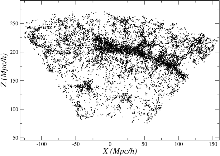
Figure 1: Projection on the $X-Z$ plane of a SDSS sample in which the Sloan Great Wall appears as a long filament of galaxies. (From [31]).

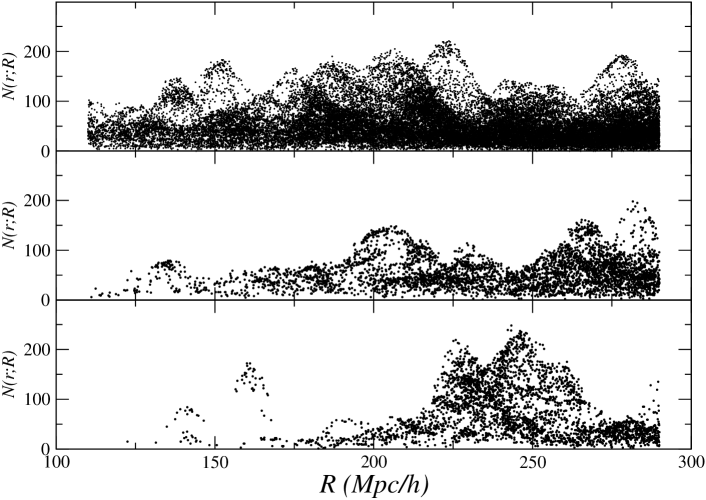
Figure 2: Behavior of $N(r;R_{i})$ in a SDSS sample and in the three different regions for $r=10$ Mpc/h (R1 top, R2 Middle and R3 bottom). (From [31]).

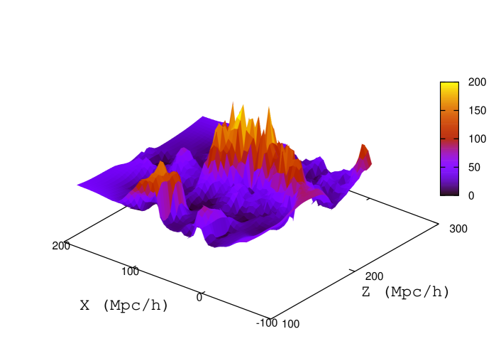
Figure 3: Three dimensional representation of the SL analysis with $r=10$ Mpc/h for R3VL2. The $x,z$ coordinates of the sphere center define the bottom plane and on the vertical axis we display the intensity of the structures, the conditional number of galaxies $N_{i}(r)$ contained in the sphere of radius $r$. The SDSS Great Wall is clearly visible as a coherent structure of large amplitude, similar to a mountain chain, extending all over the sample. (From [31]).

More information about structures amplitude and location is provided by the full $N_{i}(r)=N(r;x_{i},y_{i},z_{i})$ data, where $(x_{i},y_{i},z_{i})$ are the Cartesian coordinates of the $i^{th}$ center. In order to illustrate this point, we have chosen in Fig.3 a three dimensional representation where on the bottom plane we use the $x,z$ Cartesian coordinates of the sphere center and on the vertical axis we display the intensity of the structures, i.e. the conditional number of galaxies contained in the sphere of radius $r$. (On the $y$ direction the thickness of the sample is small, i.e. $\Delta y\approx 15$ Mpc/h). One may note that that the SDSS Great Wall is clearly visible as a coherent structure similar to a mountain chain, extending all over the sample. It is worth noticing that profiles similar to those shown in Fig.2 and Fig.3 have been found also in the 2dFGRS [33, 34] supporting the fact that these fluctuations are quite typical of galaxy distribution (see Fig.4).

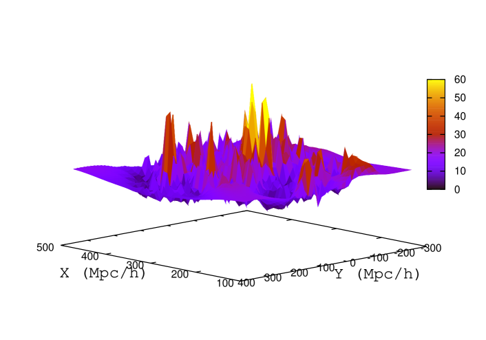
Figure 4: Analysis similar to that shown in Fig.3 but for a sample of the 2dFGRS. On the $X$ and $Y$ axes the coordinate of the center of a sphere of radius $r=10$ Mpc/h (centered on a galaxy) is reported and on the $Z$ axis the number of galaxies inside it. The mean thickness of this slice is about 50 Mpc/h. Large fluctuations in the density field are located in the correspondence of large-scale structures. (From [34]).

We now pass to the determination of the PDF of the conditional galaxy counts in spheres $P(N;r)$, at different resolution $r$, separately in two independent regions of a given sample placed at different radial distances. In a first case (left panels of Fig.5), at small scales ($r=10$ Mpc/h), the distribution is self-averaging both in the earlier data release of the SDSS (DR6 sample [52], that covers a solid angle $\Omega_{DR6}=0.94$ sr.) than in the sample extracted from the final data release (DR7 [53] with $\Omega_{DR7}=1.85$ sr. $\approx 2\times\Omega_{DR6}$ sr). Indeed, the PDF is statistically the same in the two sub-samples considered. Instead, for larger sphere radii i.e., $r=80$ Mpc/h, (right panels of Fig.5) in the DR6 sample, the two PDF show clearly a systematic difference. Not only the peaks do not coincide, but the overall shape of the PDF is not smooth and different. On the other hand, for the sample extracted from DR7, the two determinations of the PDF are in very good agreement. We conclude therefore that, in DR6 for $r=80$ Mpc/h there are large density fluctuations which are not self-averaging because of the limited sample volume [31]. They are instead self-averaging in DR7 because the volume is increased by a factor two.

The lack of self-averaging properties at large scales in the DR6 sample is due to the presence of large scale galaxy structures which correspond to density fluctuations of large amplitude and large spatial extension, whose size is limited only by the sample boundaries. The appearance of self-averaging properties in the larger DR7 sample volumes is the unambiguous proof that the lack of them is induced by finite-size effects due to long-range correlated fluctuations [50]. The lack of self-averaging does not allow one to characterize the nature of fluctuations; this is however a clear indication that the distribution has not reached spatial uniformity.

In the deepest sample we consider, which include mainly bright galaxies, the breaking of self-averaging properties does not occur as well for small $r$ but it is found for large $r$. This can be due to the same effects i.e., that the sample volumes are still too small as even in DR7 for $r=120$ Mpc/h we do not detect self-averaging properties (right panels of Fig.6). Other radial distance-dependent selections, like galaxy evolution [54], could in principle result in an effect in the same direction. Even in such a situation, our conclusion would be unchanged, i.e. on large enough scales self-averaging is broken. The reason why it is broken is then different: instead of the effect intrinsic fluctuations in the galaxy distribution, the result of a redshift-dependent effect. Because of these large fluctuations in the galaxy density field, self-averaging properties are well-defined only in a limited range of scales. Only in that range it will be statistically meaningful to measure whole-sample average quantities [31, 55].

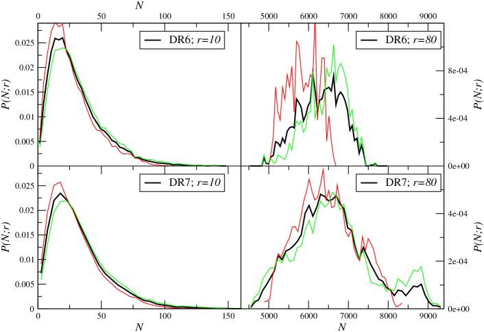
Figure 5: PDF of the conditional galaxy counts in spheres, in the sample defined by $R\in[125,400]$ Mpc/h and $M\in[−20.5,−22.2]$ in the DR6 (upper panels) and DR7 (lower panels) data, for two different values of the sphere radii $r=10$ Mpc/h and $r=80$ Mpc/h. In each panel, the black line represents the full-sample PDF, the red line (green) the PDF measured in the half of the sample closer to (farther from) the origin (From [50]).

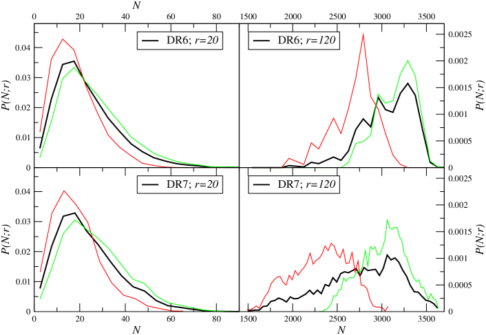
Figure 6: The same of Fig.5 but for the sample defined by $R\in[200,600]$ Mpc/h and $M\in[−21.6,−22.8]$ and for $r=20,120$ Mpc/h (From [50]).

Let us now pass to the determination of the first moment of the PDF, namely the conditional average density within radius $r$ defined as

$$\overline{n(r)}=\frac{1}{V(r)}\frac{1}{M(r)}\sum_{i=1}^{M(r)}N_{i}(r)\;,$$ (13)

where $\overline{n(r)}$ is, as discussed above, “conditioned” on the presence of the central galaxy. Then, the simplest quantity to further characterize density fluctuations is the conditional variance, or mean square deviation at scale $r$, i.e. the second moment of the PDF, which is defined as

$$\sigma^{2}(r)\equiv\mathrm{var}\,[n(r)]=\frac{1}{M(r)}\sum_{i=1}^{M(r)}n_{i}^{2}(r)-{\overline{n(r)}}^{2}\;.$$ (14)

At small length scales ($r<20$ Mpc/h) the conditional average density shows a scaling behavior with an exponent close to minus one (see Fig.7). This result is in agreement with the ones obtained by the same method in a number of different samples (see [32, 31, 33, 34] and references therein). This scaling can be interpreted as a signature of fractality of the galaxy distribution in this range of scale. In addition, this implies that the distribution is not uniform at these scales, and thus the standard two-point correlation function is substantially biased.

Then, the average conditional density (Eq.13) at larger scales ($r>20$ Mpc/h ) shows a different $r$ dependence, as can be seen in Fig.7. Our best fit is

$$\overline{n(r)}\approx\frac{0.0133}{\log r}\;,$$ (15)

that is the average density depends only weakly (logarithmically) on $r$. Alternatively, an almost indistinguishable power-law fit is provided by

$$\overline{n(r)}\approx 0.011\times r^{-0.29}\;.$$ (16)

We thus find a change of slope in the conditional average density in terms of the radius $r$ at about $\approx 20$ Mpc/h. At this point the decay of the density changes from an inverse linear decay to a slow logarithmic one. Moreover, the density $\overline{n(r)}$ does not saturate to a constant up to $\sim 80$ Mpc/h, i.e., up to the largest scales probed in this sample. Note that up to $r=80$ Mpc/h the number of points $M(r)$ is larger than $10^{4}$, so that the statistics is sufficiently robust.

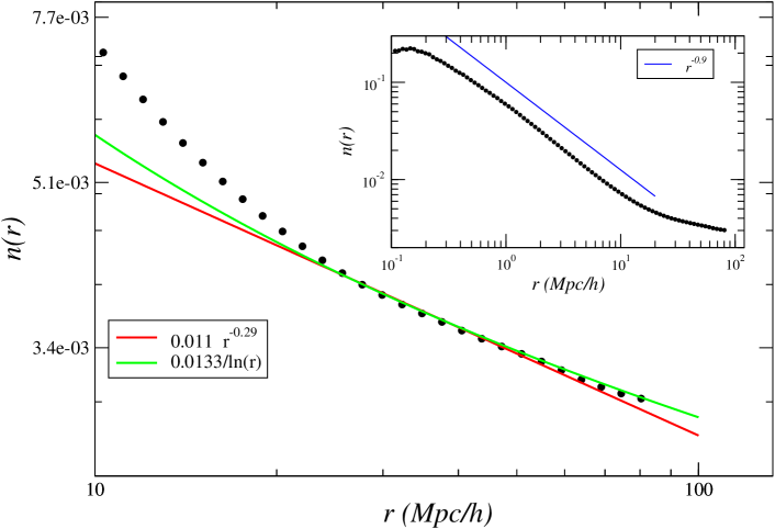
Figure 7: Conditional average density $\overline{n}(r)$ of galaxies as a function of radius. In the inset panel the same is shown in the full range of scales. Note the change of slope at $\approx 20$ Mpc/h from $1/r$ to $1/r^{0.3}$ and also the lack of flattening up to $\approx 80$ Mpc/h. (From [55]).

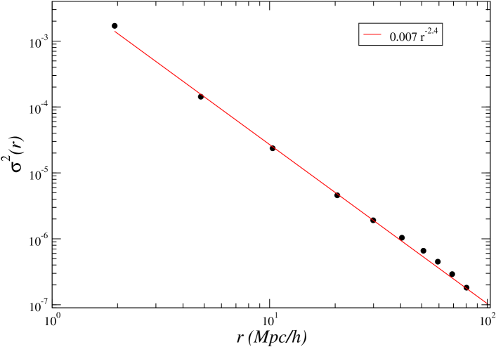
Figure 8: Variance $\sigma^{2}$ of the conditional density $n_{i}(r)$ as a function of the radius. Conversely, the corresponding variance of a Poisson point process would display a $1/r^{3}$ decay. (From [55]).

This result is in agreement with a study of the SDSS-DR4 samples [56], where, a similar change of slope was observed at about the same scale $r\approx 20$ Mpc/h, together with quite large fluctuations. Indeed, some evidences were subsequently found to support that the galaxy distribution is still characterized by rather large fluctuations up to 100 Mpc/h, making it incompatible with uniformity [33, 34, 32, 31, 57]. In the Luminous Red Galaxy (LRG) sample of SDSS, Hogg et al. [29] also found that the slope changes at $\sim$ 20 Mpc/h but then they claim to detect a transition to uniformity at about 70 Mpc/h, We do not observe in a clear way such a transition in the samples for which self-averaging properties are satisfied.

Our best fit for the variance $\sigma^{2}(r)$ of the conditional density (Eq.14) is (see Fig.8)

$$\sigma^{2}(r)\approx 0.007\times r^{-2.4}\;.$$ (17)

Given the scaling behavior of the conditional density and variance, we conclude that galaxy structures are characterized by non-trivial correlations for scales up to $r\approx 80$ Mpc/h.

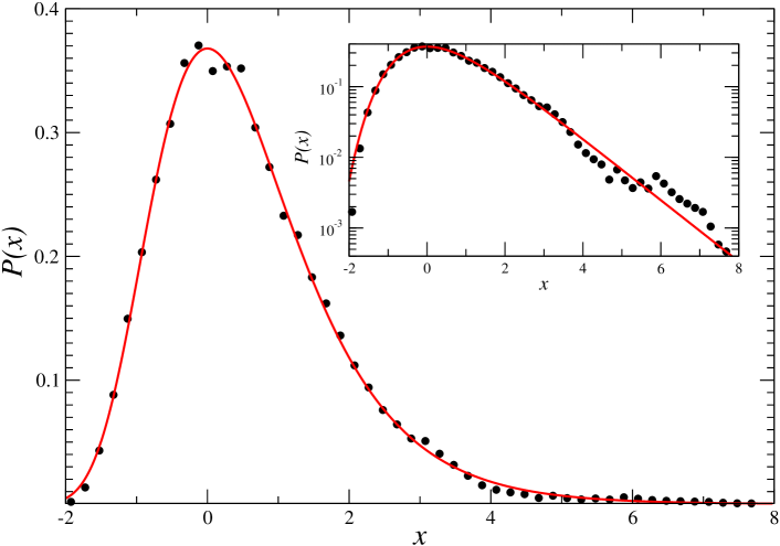
Figure 9: One of the best fits is obtained for $r=20$. The data is rescaled by the fitted parameters $\alpha$ and $\beta$. The solid line corresponds to the parameter-less Gumbel distribution Eq.20. The inset depicts the same on log-linear scale.(From [55]).

Let us now turn to the analysis of the PDF. It is well-known that away from criticality, when correlations are long-ranged and the correlation length diverges, any global (spatially averaged) observable of a macroscopic system has Gaussian fluctuations, in agreement with the central limit theorem (CLT). At criticality, however, the correlation length tends to infinity, and the CLT no longer applies. Indeed, fluctuations of global quantities in critical systems usually have non-Gaussian fluctuations. The type of fluctuations is characteristic to the universality class of the system’s critical behavior [58, 59]. Generally when correlations are long-ranged long-tailed distributions are found. In this situation some moments of the distribution may diverge as there is a finite probability to find fluctuations faraway from the most probable value [62].

To fit experimental data, the (generalized) Gumbel PDF [55] has often been used, where $a$ is a real parameter. For integer values of $a$, this distribution corresponds to the $a$-th maximal value of a random variable. The $a=1$ case corresponds to the Gumbel distribution. Experimental examples for Gumbel or generalized Gumbel distributions include power consumption of a turbulent flow [63], roughness of voltage fluctuations in a resistor (original Gumbel $a=1$ case) [61], plasma density fluctuations in a tokamak [64], orientation fluctuations in a liquid crystal [65], and other systems cited in [60]. The Gumbel distribution describing fluctuations of a global observable was first obtained analytically in [61] for the roughness fluctuations of $1/f$ noise. Its relations to extreme value statistics have been clarified [66, 67], generalizations have appeared [68], and related finite size corrections have been understood [69].

In a recent paper Bramwell [60] conjectured that only three types of distributions appear to describe fluctuations of global observables at criticality. In particular, when the global observable depends logarithmically on the system size, the corresponding distribution should be a (generalized) Gumbel. For example the mean roughness of $1/f$ signals depends on the logarithm of the observation time (system size), and the corresponding PDF is indeed the Gumbel distribution [61].

The Gumbel (also known as Fisher-Tippet-Gumbel) distribution is one of the three extreme value distribution [70, 71]. It describes the distribution of the largest values of a random variable from a density function with faster than algebraic (say exponential) decay. When fluctuations are characterized by the Gumbel PDF the situation is in between the Gaussian case, where all moments are well-defined, and the case in which the tail of the PDF scales as a power-law, i.e. the case in which several moments of the PDF may diverge corresponding to an is extremely wild fluctuation field. It is important to stress that models of galaxy formation predict Gaussian-like fluctuations on sufficiently large scales. The key-issue concerns indeed at which scales fluctuations show a Gaussian behavior, which is a closely related problem to the scale at which the distribution turns to spatial uniformity [31, 32].

The Gumbel distribution’s PDF is given by

$$P(y)=\frac{1}{\beta}\exp\left[-\frac{y-\alpha}{\beta}-\exp\left(-\frac{y-\alpha}{\beta}\right)\right]\;.$$ (18)

With the scaling variable

$$x=\frac{y-\alpha}{\beta}$$ (19)

the density function (Eq.18) simplifies to the parameter-free Gumbel

$$P(x)=e^{-x-e^{-x}}$$ (20)

with (cumulative) distribution $e^{-e^{-x}}$. Note that this distribution corresponds to large extremes, while for low extreme values, $x$ is used instead of $-x$ in the Gumbel distribution.

The mean and the standard deviation (variance) of the Gumbel distribution (Eq.18) are respectively

$$\mu=\alpha+\gamma\beta,\quad\sigma^{2}=(\beta\pi)^{2}/6$$ (21)

where $\gamma=0.85772\dots$ is the Euler constant. For the scaled Gumbel (Eq.20) the first two cumulants of Eq.21 simplify to $\gamma$ and $\pi^{2}/6$.

To probe the whole distribution of the conditional density $n_{i}(r)$, we fitted the Gumbel distribution (Eq.18) via its two parameters $\alpha$ and $\beta$. One of our best fits is obtained for $r=20$ Mpc/h, see Fig. 9. The data, moreover, convincingly collapses to the parameter-less Gumbel distribution (Eq.20) for all values of $r$ for $10\leq r\leq 80$ Mpc/h, with the use of the scaling variable $x$ from Eq.19 (see Figs. 10-11). Note that for a Poisson point process (uncorrelated random points) the number $N(r)$ (and consequently also the density) fluctuations are distributed exactly according to a Poisson distribution, which in turn converges to a Gaussian distribution for large average number of points $\overline{N(r)}$ per sphere. In our samples, $\overline{N(r)}$ is always larger than 20 galaxies, where the Poisson and the Gaussian PDFs differ less than the uncertainty in our data. Note also that due to the central limit theorem, all homogeneous point distributions (not only the Poisson process) lead to Gaussian fluctuations. Hence the appearance of the Gumbel distribution is a clear sign of inhomogeneity and large scale structures in our samples.

The fitting parameters in Eq.18 varied with the radius $r$ approximately as

$$\alpha\approx\frac{0.007}{r^{0.21}},\quad\beta\approx\frac{0.035}{r}\;.$$ (22)

although a logarithmic fit $\alpha\approx 0.0115/\log r$ cannot be excluded either. With the fitted values of $\alpha$ and $\beta$ we recover the (directly measured) average conditional density of galaxies through Eq. 21. On the other hand, we have a discrepancy when comparing the directly measured $\sigma^{2}$ to that obtained from the Gumbel fits through Eq. 21. The reason for this discrepancy is that the uncertainty in the tail of the PDF $P(n,r)$ is amplified when we directly calculate the second moment.

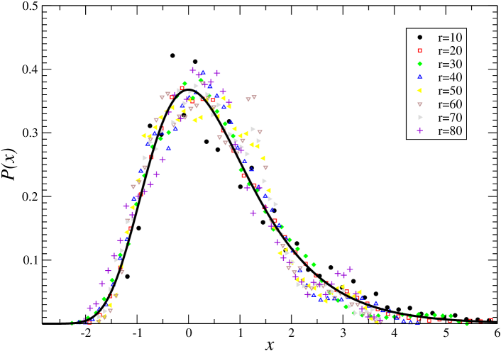
Figure 10: Data curves of different $r$ scaled together by fitting parameters $\alpha$ and $\beta$ for each curves. The solid line is the parameter-free Gumbel distribution Eq.20. (From [55]).

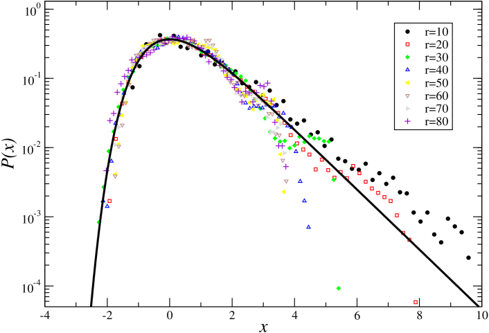
Figure 11: The same as Fig. 10, but on log-linear scale to emphasize the tails of the distribution.(From [55]).

Due to the scaling and data collapse we argued that the large scale galaxy distribution shows similarities with critical systems [55]. Here the galaxy density around each galaxy is analogous to a random variable describing a spatially averaged quantity in a volume. The average conditional galaxy density depends on the volume size ($\sim r^{3}$) only logarithmically $\overline{n(r)}\sim 1/\log r$ from Eq.15. According to the conjecture of Bramwell for critical systems [60], if a spatially averaged quantity depends only weakly (say logarithmically) on the system size, the distribution of this quantity follows the Gumbel distribution. This is indeed what we see in the galaxy data. Hence our two observations about the average density and the density distribution are compatible with the behavior of critical systems in statistical physics. We note that standard models of galaxy formation predict homogeneous mass distribution beyond $\approx 10$ Mpc/h [47, 32, 31]. To explain our findings about non-Gaussian fluctuations up to much larger scales presents a challenge for future theoretical galaxy formation models (see [47, 32, 31, 33, 34, 55] for more details).

3 Assumptions and basic principles in cosmology

As we noticed in the introduction, a widespread idea in cosmology is that the so-called concordance model of the universe combines two fundamental assumptions. The first is that the dynamics of space-time is determined by Einstein’s field equations. The second is that the universe is homogeneous and isotropic. This hypothesis, usually called the Cosmological Principle, is though to be a generalization of the Copernican Principle that “the Earth is not in a central, specially favored position” [72, 73]. The FRW model is derived under these two assumptions and it describes the geometry of the universe in terms of a single function, the scale factor, which obeys to the Friedmann equation [1]. There is a subtlety in the relation between the Copernican Principle (all observes are equivalent and there are no special points and directions) and the Cosmological Principle (the universe is homogeneous and isotropic). Indeed, the fact that the universe looks the same, at least in a statistical sense, in all directions and that all observers are alike does not imply spatial homogeneity of matter distribution. It is however this latter condition that allows us to treat, above a certain scale, the density field as a smooth function, a fundamental hypothesis used in the derivation of the FRW metric. Thus there are distributions which satisfy the Copernican Principle and which do not satisfy the Cosmological Principle [26]. These are statistically homogeneous and isotropic distributions which are also spatially inhomogeneous . Therefore the Cosmological Principle represents a specific case, holding for spatially homogeneous distributions, of the Copernican Principle which is, instead, much more general. Statistical and spatial homogeneity refer to two different properties of a given density field. The problem of whether a fluctuations field is compatible with the conditions of the absence of special points and direction can be reformulated in terms of the properties of the probability density functional (PDF) which generates the stochastic field.

Matter distribution in cosmology then is considered to be a realization of a stationary stochastic point process. This is enough to satisfy the Copernican Principle i.e., that there are no special points or directions; however this does not imply spatial homogeneity. Spatially homogeneous stationary stochastic processes satisfy the special and stronger case of the Copernican Principle described by Cosmological Principle. Indeed, isotropy around each point together with the hypothesis that the matter distribution is a smooth function of position i.e., that this is analytical, implies spatial homogeneity. (A formal proof can be found in [75].) This is no longer the case for a non-analytic structure (i.e., not smooth), for which the obstacle to applying the FRW solutions has in fact solely to do with the lack of spatial homogeneity [77].

The condition of spatial homogeneity (uniformity) is satisfied if the ensemble average density of the field $\langle\rho\rangle$ is strictly positive. We discussed in the previous sections tests to establish whether a point distribution in a given sample (i.e. galaxies) is spatially uniform. The additional test provided by the analysis of the PDF of conditional fluctuations in disjointed sub-samples, i.e. Eq.12, allows us to determine a distribution is also statistically stationary. In the case in which systematic differences are found to be important one may then further test whether this is due to the breaking of self-averaging properties for the presence of large-scale fluctuations or whether this is due to the lack of translational invariance. A statistical test able to distinguish between these two cases, can also give an information about the validity of the Copernican principle as we discuss in the next section .

3.1 Testing the Copernican and cosmological principles

Let us firstly consider a case where translational invariance is broken. We generate a Poisson-Radial distribution (PRD) which is a inhomogeneous distribution that can mimic the effect of a “local hole” around the origin. In a sphere of radius $R_{0}=1$ we place, for instance, $N=2\cdot 10^{5}$ points. In each bin at radial distance from the sphere center $[R_{i},R_{i+1}]$, and with thickness $\Delta R$, the distribution is Poissonian with a density varying as $n(R)=n_{0}\cdot R\;,$ where $n_{0}$ is a constant. We determine the PDF $P(N;r)$ of conditional fluctuations obtained by making an histogram of the values of $N(r;R)$ at fixed $r$ (see the upper panels of Fig.12). The whole-sample PDF is clearly left-skewed: this occurs because the peak of the PDF corresponds to the most frequent counts which are at large radial distance simply because shells far-way from the origin contain more points. The spread of the PDF can easily be related to the difference in the density between small and large radial distances in the sample. By computing the PDF into two non-overlapping sub-samples, nearby to and faraway from the origin, one may clearly identify the systematic dependence of this quantity on the specific region where this is measured. This breaking of the self-averaging properties is caused by the radial-distance dependence of the density and thus by the breaking of translational invariance (as noticed above in the data a redshift dependent selection effect may cause in the same result).

Let us now consider a stationary stochastic distribution, where the breaking self-averaging properties is due to the effect of large scale fluctuations. An example is represented by the inhomogeneous toy model (ITM) constructed as follows. We generate a stochastic point distribution by randomly placing, in a two-dimensional box of side $L$, structures represented by rectangular sticks. We first distribute randomly $N_{s}$ points which are the sticks centers: they are characterized by a mean distance $\Lambda\approx(L^{3}/N_{s})^{1/3}$. Then the orientation of each stick is chosen randomly. The points belonging to each stick are also placed randomly within the stick area, that for simplicity we take to be $\ell\times\ell/10$. The length-scale $\ell$ can vary, for example being extracted from a given PDF. The number of sticks placed in the box fixes $\Lambda$. This distribution is by construction stationary i.e., there are no special points or directions. When $\ell\geq L$ and $\Lambda\leq L$ but with $\ell$ varying in such a way that there can been large differences in its size, the resulting distribution is long-range correlated, spatially inhomogeneous and it can be not self-averaging. This latter case occurs when, by measuring the PDF of conditional fluctuations in different regions of a given sample, one finds, for large enough $r$, systematic differences in the PDF shape and peak location (see the bottom panels Fig.12). These are due to the strong correlations extending well over the size of the sample.

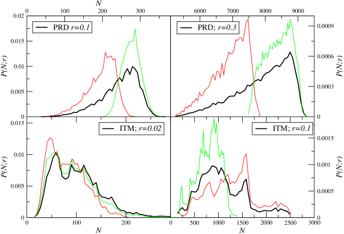
Figure 12: Upper panels: The PDF for $r=0.1$ (left) and $r=0.3$ (right) for PRD computed for the whole sample (black line). The red (green) line shows the PDF measured in the sub-sample placed closer to (father from) the origin. Lower Panels: The same for the ITM at scales $r=0.02$ (left) and $r=0.1$ (right) (From [50].

How can we distinguish between the case in which a distribution is not self-averaging because it is not statistically translational invariant and when instead this is stationary but fluctuations are too extended in space and have too large amplitude ? The clearest test is to change the scale $r$ where $P(N,r)$ is measured, and determining whether the PDF is self-averaging. Indeed, in the case of the PRD the strongest differences between the PDF measured in regions placed at small and large radial distance from the structure center, occur for small $r$. This is because the local density has the largest variations at small and large radial distances by construction. When $r$ grows, different radial scales are mixed as the generic sphere of radius $r$ pick up contributions both from points nearby the origin and from those far away from it, resulting in a smoothing of local differences. Instead, in the ITM for small $r$ the difference is negligible while for large enough $r$ the different determinations of the local density start to feel the presence of a few large structures which dominate the large scale distribution in the sample.

3.2 Implications for theoretical modeling

The discussion in the previous sections was meant to treat the statistical properties of the galaxy density field in a spatial hyper-surface. As mentioned above, this is an approximation valid when considering the galaxy distribution limited to relatively low redshifts, i.e. $z<0.2$. In particular, we have developed a test to focus on the properties of statistical and homogeneity homogeneity in nearby redshift surveys. The assumptions of the cosmological model enter in the data analysis when calculating the metric distance from the redshift and the absolute magnitude from the apparent one and the redshift. However, given that second order corrections are small for $z<0.2$, our results are basically independent on the chosen underlying model to reconstruct metric distances and absolute magnitudes from direct observables. In practice we can use just a linear dependence of the metric distance on the redshift (which is, to a very good approximation, compatible with observations at low redshift). For this same reason we can approximate the observed galaxies as lying in a spatial hyper-surface.

In the ideal case of having a very deep survey, up to $z\approx 1$, we should consider that we make observations on our past light-cone which is not a space-like surface. In order to evolve our observations onto a spatial surface we would need a cosmological model, which at such high redshift can play an important role in the whole determination of statistical quantities. A sensible question is whether we can to reformulate the statistical test given so that it can be applied to data on our past light-cone, and not on an assumed spatial hyper-surface. Going to higher redshift poses a number of question, first of the all the one of checking the effect of the assumptions used to construct metric distances and absolute magnitudes from direct observables. Testing these effects can be simply achieved by using different distance-redshift relations.

However, we note that a smooth change of the distance-redshift relation as implied by a given cosmological model, may change the average behavior of the conditional density as a function of redshift but it cannot smooth out fluctuations, i.e. it cannot substantially change the PDF of conditional fluctuations when they are measured locally. Indeed, our test is based on the characterization of the PDF of conditional fluctuations and not only of the behavior of the conditional average density as a function of distance. The PDF provides, in principle, with a complete characterization of the fluctuations statistical properties. We have shown that the PDF of fluctuations has a clear imprint when the distribution is spherically symmetric or when it is spatially inhomogeneous but statistically homogeneous.

The fact that we analyze conditional fluctuations means that we consider only local properties of the fluctuations: local with respect to an observer placed at different radial (metric) distances from the us, i.e. at different redshifts. For the determination of the PDF we have to consider two different length scale: the first is the (average) metric distance $R$ of the galaxies on which we center the sphere and the second is the sphere radius $r$. Irrespective of the value of $R$ when $r$ is smaller than a few hundreds Mpc (i.e., when its size is much smaller than any cosmological length scale), we can always locally neglect the specific $R(z)$ relation induced by a specific cosmology. In other words, when the sphere radius is limited to a few hundreds Mpc we can approximate the measurements of the conditional density to be performed on a spatial hyper-surface.

The whole description of the matter density field in terms of FRW or even Lemaitre-Tolman-Bondi (LTB) cosmologies, refer to the behavior of, for instance, the average matter density as a function of time (in the LTB case also as a function of scale) but it says anything on the fluctuation properties of the density field. Thus, when looking at different epochs in the evolution of the universe, we should detect that the average density varies (being higher in early epochs). This means only that the peak of the PDF will be located at different $N$ values, but the shape of the PDF is unchanged by this overall (smooth) evolution. Fluctuations are simply not present in the FRW or LTB models, and the whole issue of back-reaction studies is to understand what is their effect.

Note that models which explain dark energy through inhomogeneity do so using a spatial under-density in the matter density which varies on Gpc scales — out to $z\approx 1$ [76]. These models by placing us at the center of the universe, violate the Copernican Principle. In this respect we note that, while we cannot make any claim for $z>0.2$ based on current data, the fact that galaxy distribution is spatially inhomogeneous but statistically homogeneous up to 100 Mpc/h, already poses intriguing theoretical problems. Indeed, in that in that range of scales, the modeling of the matter density field as a perfect fluid, as required by the FRW models, is not even a rough approximation. As pointed out by various authors [27, 79], if the linearity of the Hubble law is a consequence of spatial homogeneity, how is it that observations show that it is very well linear at the same scales where matter distribution is inhomogeneous ? Recently [78] it was speculated a solution to this apparent paradox can be found by considering both the effects of back-reaction and the synchronization of clocks. While this is certainly an interesting approach, the formulation of a more complete and detailed theoretical framework is still lacking.

Finally we note that there are several complications in radially inhomogeneous models at high redshift. Beyond the change of the distance-redshift relation, discussed above, another is how structure evolves from our past light-cone onto a surface of constant time. Thus in order to make a precise test on the spatial properties of a given model, one needs to develop the corresponding theory of structure formation. However, at least at low redshifts, it seems implausible that the main feature of the model, the specific redshift-dependence of the spatial density, will not be the clearer prediction for the observations of galaxy structures.

4 Conclusions

We discussed several results showing that galaxy distribution in the newest galaxy samples is characterized by large fluctuations. These are manifest in the scaling properties of the conditional density which shows scaling behaviors. Particularly at small scales this statistics presents a power-law behavior with an exponent close to minus one, corresponding to a fractal dimension $D\approx 2$. The difference with the different dimension $D=1.2$ reported by authors (see e.g. [18, 19, 20]) is due to the finite size effects which perturb the estimation of the two-point correlation function $\xi(r)$ [26].

On larger scales and up to $r\approx 80$ Mpc/h a smaller correlation exponent is found to fit the data: the density depends, for $20\leq r\leq 80$ Mpc/h, only weakly (logarithmically) on the system size. Correspondingly, we find that the density fluctuations follow the Gumbel distribution of extreme value statistics. This distribution is clearly distinguishable from a Gaussian distribution, which would arise for a homogeneous spatial galaxy configuration. While in the Gaussian case the rapid decay of the tails of the distribution cut large fluctuations, in the Gumbel case the large value tail decays slower. In such a situation the density field is still inhomogeneous, although not as wild as in the case in which the PDF presents power-law tails.

We discussed that in several samples it is found that self-averaging properties, at large scales, are not satisfied. This is due to the presence of large scale galaxy structures which correspond to density fluctuations of large amplitude and large spatial extension, whose size is limited only by the sample boundaries. Note that the lack of self-averaging does not allow one to characterize the nature of fluctuations; this is however a clear indication that the distribution has not reached spatial uniformity.

The large scale inhomogeneities detected in the three dimensional galaxy samples are at odds with the predictions of standard models. In particular according to these models the density field should present on large scales sub-Poissonian fluctuations, or a super-homogeneous nature with negative correlations [48, 26]. Forthcoming redshift surveys will allow us to clarify whether on such large scales galaxy distribution is still inhomogeneous but statistically stationary, or whether the evidences for the breaking of spatial translational invariance found in the galaxy samples considered were due to selection effects in the data.

Finally we discussed that the galaxy distribution is found to be compatible with the assumptions that this is transitionally invariant, i.e. it satisfies the requirement of the Copernican Principle that there are no spacial points or directions., while because of lack of spatial homogeneity galaxy distribution is not compatible with the stronger assumption of spatial homogeneity, encoded in the Cosmological Principle.

Acknowledgments

We are in debt with T. Antal, Y. Baryshev and N. L. Vasilyev for fruitful collaborations. We also thank A. Gabrielli and M. Joyce for interesting discussions. We acknowledge the use of the Sloan Digital Sky Survey data (http://www.sdss.org).

References

- [1] Weinberg S 2008 Cosmology (Oxford University Press, Oxford)
- [2] Weinberg S 1989 Rev.Mod.Phys. 61 1
- [3] Einasto J Unesco Eolss Encyclopedia astro-ph/0901.0632
- [4] Buchert T 2008 Gen.Rel.Grav. 40 467
- [5] Wiltshire D L 2007 Phys.Rev.Lett. 99 251101
- [6] de Vaucouleurs G 1970 Science 167 1203
- [7] Huchra J et al. 1983 Astrophys.J.Suppl. 52 89
- [8] Falco E F et al. 1999 Pub.Astron.Soc.Pac. 111 438
- [9] Giovanelli R and Haynes M P 1993 Astronom.J. 105 1271
- [10] da Costa L et al. 1988, Astrophys.J.S 327 544
- [11] Shectman S A et al., 1996, Astrophys.J.S 470 172
- [12] Colless M et al. 2001 Mon.Not.R.Acad.Soc 328 1039
- [13] York D et al. 2000 Astronom.J. 120 1579
- [14] de Lapparent V Geller M J and Huchra J P 1986 Astrophys.J. 302 1
- [15] Geller M and Huchra J 1989 Science 246 897
- [16] Gott J R III et al., 2005 Astrophys.J. 624 463
- [17] Totsuji H and Kihara T 1969 Pub.Astron.Soc.Jap. 21 221
- [18] Davis M and Peebles P J E 1983 Astrophys.J. 267 465
- [19] Davis M et al. 1988 Astrophys.J.Lett. 333 L9
- [20] Park C et al. 1994 Astrophys.J. 431 569
- [21] Benoist C et al. 1996 Astrophys.J. 472 452
- [22] Norberg E 2001 Mon.Not.R.Acad.Soc. 328 64
- [23] Norberg E 2002 Mon.Not.R.Acad.Soc. 332 827
- [24] Zehavi I et al. 2002 Astrophys.J. 571 172
- [25] Zehavi I et al. 2004 Astrophys.J. 608 16
- [26] Gabrielli A Sylos Labini F Joyce M and Pietronero L 2005, Statistical Physics for Cosmic Structures (Springer Verlag, Berlin)
- [27] Sylos Labini F et al. 1998 Phys.Rep. 293 66
- [28] Wu K K Lahav O and Rees M 1999 Nature 225 230
- [29] Hogg D W et al. 2005 Astrophys.J. 624 54
- [30] Baryshev Yu and Teerikorpi P 2006 Bull.Spec.Astr.Obs. 59 92
- [31] Sylos Labini F Vasilyev N L Baryshev Y V 2009 Astron.Astrophys 508, 17
- [32] Sylos Labini F et al. 2009 Europhys.Lett. 86 49001
- [33] Sylos Labini F Vasilyev N L Baryshev Y V 2009 Europhys.Lett. 85 29002
- [34] Sylos Labini F Vasilyev N L Baryshev Y V 2009 Astron.Astrophys. 496 7
- [35] Pietronero L 1987 Physica A 144 257
- [36] Coleman P and Pietronero L 1992 Phys.Rep. 213 311
- [37] Gabrielli A and Sylos Labini F 2001 Europhys.Lett. 54 286
- [38] Picard A 1991Astronom.J. 102 445
- [39] Busswell G S et al 2004 Mon.Not.R.Acad.Soc 354 991
- [40] Frith W J 2003 Mon.Not.R.Acad.Soc 345 1049
- [41] Frith W J 2006 Mon.Not.R.Acad.Soc 371 1601
- [42] Kerscher M et al. 1998 Astron.Astrophys. 333 1
- [43] Chiaki H et al 2003 Publ.Astron.Soc.Jap. 55 911
- [44] Peacock J A 1999 Cosmological physics (Cambridge University Press, Cambridge)
- [45] Spergel D N et al 2007 Astrophys.J.Suppl. 170 377
- [46] Springel V et al 2005 Nature 435 629
- [47] Sylos Labini F and Vasilyev N L 2008 Astron.Astrophys 477 381
- [48] Gabrielli A Joyce M Sylos Labini F 2002 Phys.Rev. D65 083523
- [49] Gabrielli A et al 2003 Phys.Rev. D67 043406
- [50] Sylos Labini F and Baryshev Y V 2010 J.Cosmol.Astropart.Phys. JCAP06(2010)021
- [51] Aharony A and Harris B 1996 Phys.Rev.Lett. 77 3700
- [52] Adelman-McCarthy J K et al 2008 Astrophys.J.Suppl. 175 297
- [53] Abazajian K et al 2009 Astrophys.J.Suppl. 182 543
- [54] Loveday J 2004 Mon.Not.R.Acad.Soc 347 601
- [55] Antal T Sylos Labini F Vasilyev N L Baryshev Y V 2009 Europhys.Lett. 88 59001
- [56] Sylos Labini F Vasilyev N L Baryshev Y V 2007 Astron.Astrophys. 465 23
- [57] Sylos Labini F et al 2009 Astron.Astrophys. 505 981
- [58] Foltin G et al 1994 Phys. Rev. E 50 R639
- [59] Rácz Z in ”Slow Relaxations and Nonequilibrium Dynamics in Condensed Matter” J-L Barrat et al eds (Springer-Verlag, 2002) cond-mat/0210435
- [60] Bramwell S T 1998 Nature 396 552
- [61] Antal T Droz M Györgyi G Rácz Z 2001 Phys.Rev.Lett., 87 240601.
- [62] Bouchaud J-P and Potters M 1999 Theory of Financial Risks (Cambridge University Press, Cambridge) cond-mat/9905413
- [63] Bramwell S T 1998 Nature 396 552
- [64] Van Milligen B P et al 2005 Phys.Plasmas 12 052507
- [65] Joubaud S et al 2008 Phys.Rev.Lett., 100 180601
- [66] Bertin E 2005 Phys.Rev.Lett. 95 170601
- [67] Bertin E and Clusel M 2006 J.Phys.A 39 7607
- [68] Antal T Droz M Györgyi G Rácz Z 2002 Phys.Rev.E 65 046140
- [69] Györgyi G Moloney N R Ozogány K Rácz Z 2008 Phys.Rev.Lett. 100 210601
- [70] Fisher R A Tippett L H C 1928 Cambridge Phil. Soc. 28 180
- [71] Gumbel E J 1958 Statistics of Extremes (Columbia University Press)
- [72] Bondi H 1954 Cosmology, (Cambridge University Press, Cambridge.
- [73] Clifton T and Ferreira P G 2009 Phys.Rev. D80 103503
- [74] Mandelbrot B B 1983 The Fractal Geometry of Nature (Freeman, New York)
- [75] Straumann N 1977 Helv.Phys.Acta 47 379
- [76] Clifton T Ferreira P G Land K 2008 Phys.Rev.Lett. 101 131302
- [77] Joyce M et al 2000 Europhys.Lett. 50 416
- [78] Wiltshire D L 2009 Phys.Rev.D 80 123512
- [79] Wiltshire D L 2008 Int.J.Mod.Phys. 17 641