Scaling Analysis in the Numerical Renormalization Group Study of the Sub-Ohmic Spin-Boson Model

Abstract

The spin-boson model has nontrivial quantum phase transitions in the sub-Ohmic regime. For the bath spectra exponent $0\leqslant s<1/2$, the bosonic numerical renormalization group (BNRG) study of the exponents $\beta$ and $\delta$ are hampered by the boson-state truncation, which leads to artificial interacting exponents instead of the correct Gaussian ones. In this paper, guided by a mean-field calculation, we study the order-parameter function $m(\tau=\alpha-\alpha_{c},\epsilon,\Delta)$ using BNRG. Scaling analysis with respect to the boson-state truncation $N_{b}$, the logarithmic discretization parameter $\Lambda$, and the tunneling strength $\Delta$ are carried out. Truncation-induced multiple-power behaviors are observed close to the critical point, with artificial values of $\beta$ and $\delta$. They cross over to classical behaviors with exponents $\beta=1/2$ and $\delta=3$ on the intermediate scales of $\tau$ and $\epsilon$, respectively. We also find $\tau/\Delta^{1-s}$ and $\epsilon/\Delta$ scalings in the function $m(\tau,\epsilon,\Delta)$. The role of boson-state truncation as a scaling variable in the BNRG result for $0\leqslant s<1/2$ is identified and its interplay with the logarithmic discretization revealed. Relevance to the validity of quantum-to-classical mapping in other impurity models is discussed.

I Introduction

The spin-boson model is the simplest model that describes a quantum two-level system subjected to the influence of a dissipative environment. It has applications in various fields in physics Weiss1 and its properties are studied extensively. Leggett1 Especially, for the bath spectra exponent $0\leqslant s<1$ (sub-Ohmic bath), the ground state of the spin-boson model may change from the spin-tunneling state to the spin-pinned state through a second-order phase transition, as the dissipation strength crosses a critical value from below. This environment-induced quantum phase transition attracts much attention in the past few years. Kehrein1 ; Bulla1 ; Vojta1 ; Tong1 ; Bulla2

Among the many theoretical methods that have been used to study this quantum phase transition, the bosonic numerical renormalization group (NRG) method is regarded as the most accurate one. Technically, NRG is composed of three standard procedures: logarithmic discretization, transforming the Hamiltonian into a semi-infinite chain, and the iterative diagonalization. Thanks to the logarithmic discretization, the state information at exponentially small energy scales is kept along the iterative diagonalization. Therefore, NRG allows for reliable extraction of critical exponents and description of the crossover behavior. Two parameters control the precision of NRG, i.e., the logarithmic discretization $\Lambda$ ($\Lambda>1$) and the number of kept states $M_{s}$. The original Wilson’s NRG is designed for the impurity problem with a fermionic bath. Wilson1 In the past few years, the extension of NRG to impurity models with bosonic bath, such as the spin-boson model, proved to be fruitful. Bulla1 ; Lee1 ; Tornow1 Due to the infinite local Hilbert space for each bosonic bath mode, one has to truncate the space into $N_{b}$ states. Usually the boson occupation states are used as the local bases, although optimal bases have also been considered. Bulla1 Using this bosonic NRG (BNRG), the thermodynamical as well as dynamical quantities for the spin-boson model are studied and the critical exponents in the sub-Ohmic regime obtained. Although it was clear that the localized fixed point ($\langle\sigma_{z}\rangle\not=0$) cannot be described exactly due to the truncation of boson states, it was believed and partly checked Bulla1 ; Vojta1 that the BNRG shares the virtue of NRG, i.e, the parameters $\Lambda$, $M_{s}$, and $N_{b}$ only influences the value of non-universal quantities, such as the critical point value $\alpha_{c}$ and the prefactors of power laws. The exact value of them can be reliably obtained by extrapolating $\Lambda\rightarrow 1$, $M_{s}\rightarrow\infty$, and $N_{b}\rightarrow\infty$. The universal quantities such as the critical exponents are not supposed to depend on $\Lambda$, $M_{s}$, or $N_{b}$.

For the quantum critical behavior of the spin-boson model in the sub-Ohmic regime, the following critical exponents have been studied Bulla1 ; Vojta1 :

$$m(\alpha>\alpha_{c},T=0,\epsilon=0)\propto\left(\alpha-\alpha_{c}\right)^{\beta}\!\!$$

$$m(\alpha=\alpha_{c},T=0,\epsilon)\propto\epsilon^{1/\delta}\!\!$$

$$\chi(\alpha,T=0,\epsilon=0)\propto|\alpha-\alpha_{c}|^{-{\gamma}}$$

$$T^{*}(\alpha,\epsilon=0)\propto|\alpha-\alpha_{c}|^{z\nu}$$

$$\chi(\alpha=\alpha_{c},T,\epsilon=0)\propto T^{-x}$$

$$C(\omega)(\alpha=\alpha_{c},T=0,\epsilon=0)\propto\omega^{-y}$$ (1)

Here, $\alpha$ and $\epsilon$ describe the coupling strength between the spin and bosons, and the bias field on the spin, respectively. $\chi$ and $C(\omega)$ are static susceptibility and dynamical spin correlation function, respectively. The naive BNRG study of these critical exponents leads to the following conclusions. Bulla1 ; Vojta1 (i) In the regime $0\leqslant s<1$, the critical fixed points are interacting and the corresponding critical exponents are non-classical; and (ii) The hyperscaling relation and $\omega/T$ scaling hold. In the regime $0\leqslant s<1/2$, these conclusions are in contrast to previous theories based on the quantum-to-classical mapping. There, the spin-boson model is mapped into a one-dimensional Ising model with $J_{ij}\propto 1/(r_{i}-r_{j})^{(1+s)}$. Leggett1 In the regime $0\leqslant s<1/2$, this Ising model is above its upper critical dimension, leading to Gaussian critical fixed point and classical exponents. The hyperscaling relation and $\omega/T$ scaling do not hold there. Dyson1 ; Fisher1 ; Luijten1 Recently, using a number of new methods, Winter1 ; Alvermann1 ; Wong1 ; Zhang1 ; Lv1 the quantum phase transition in the sub-Ohmic spin-boson model has been studied. The obtained critical coupling strength $\alpha_{c}(s)$,Winter1 ; Alvermann1 ; Wong1 ; Zhang1 ; Lv1 the exponent $\nu$, Winter1 and $\gamma$ (Ref. Alvermann1, ) are consistent with the BNRG results. However, the quantum Monte Carlo (QMC) simulation Winter1 and the exact diagonalization study Alvermann1 found that in the regime $0\leqslant s<1/2$, the critical point is Gaussian with classical exponent $\beta=1/2$, being different from the BNRG conclusion. In the regime $1/2\leqslant s<1$, BNRG results are consistent with the quantum-to-classical mapping theory which predicts an interacting fixed point and $\omega/T$ scaling.

Recently, a closer examination of BNRG method discloses two sources of error, which were not noticed before. One is the boson state truncation error, Vojta2 the other is the mass-flow error. Vojta2 ; Vojta3 The boson state truncation error spoils the evaluation of the order-parameter related exponents $\beta$ and $\delta$, while the mass-flow problem influences the correct evaluation of $x$. The two sources of error are different in nature and exist simultaneously in the BNRG algorithm in the whole regime $0\leqslant s<1$. But, they influence the critical behavior only in the regime $0\leqslant s<1/2$, where the critical fixed point is expected to be Gaussian in the absence of these errors.

For the mean-field spin-boson model which has a Gaussian critical fixed point, Hou1 we showed that the boson state truncation leads to an artificial interacting fixed point in the regime $0\leqslant s<1/2$, but has no influence in $1/2\leqslant s<1$. This is an example where the boson-state truncation destroys the Gaussian fixed point and spoils the correct calculation of the exponents $\beta$ and $\delta$. It leads to the surmise that the same may happen in the BNRG study of the spin-boson model. It would be difficult to find the Gaussian nature of the critical fixed point in $0\leqslant s<1/2$ using BNRG, if the truncation works the same way as in the mean-field Hamiltonian.

In Ref. Vojta2, , the boson-state truncation error is traced back to the presence of a dangerously irrelevant variable for a Gaussian critical fixed point. The correct exponent can be seen on the intermediate scales. For the more fundamental problem of mass- flow error, Vojta et al. Vojta3 have proposed an extended NRG algorithm to partly remedy the problem and got the correct exponent $x=1/2$ in $0\leqslant s<1/2$. In this paper, we focus on the boson state truncation error. In the BNRG, it is still unclear how a finite $N_{b}$ leads to wrong $\beta$ and $\delta$, and how to extract the correct exponents. For the spin-boson model, a thorough numerical study in the regime $0\leqslant s<1/2$ is required to prove or disprove the validity of the quantum-to-classical mapping in this model.Winter1 ; Alvermann1 ; Vojta2 ; Vojta3 ; Kirchner1 ; Florens1 Here, we use the scaling approach to analyze the BNRG data with respect to boson-state truncation $N_{b}$, logarithmic discretization parameter $\Lambda$, and tunneling strength $\Delta$. We find that for any finite $N_{b}$, the order parameter $m$ has a multiple power form like that at the tricritical point, Hankey1 with nonclassical exponents $\beta$ and $\delta$ dominated by the discretization scheme. The correct power- law behavior can be observed on the intermediate scale away from the critical point. These two different power-law regimes are connected at a crossover scale, which goes to zero as a power of $x=1/N_{b}$ and $w=\Lambda-1$. Thus, in the limit of either $x\rightarrow 0$ or $w\rightarrow 0$, the classical critical exponents $\beta$ and $\delta$ are recovered. This is the same as in the mean-field spin-boson model, which we will detail in the Appendix. Besides, we also disclose the role of $\Delta$ as a scaling variable in the order parameter close to criticality.

In Sec. II, the spin-boson model and our main results are presented. In Sec. III, a summary and discussion will be made. In the Appendix, we present the critical behavior of order parameter and susceptibility for the mean-field spin-boson model.

II Model and Results

The Hamiltonian of the spin-boson model reads as

$$H=-\frac{\Delta}{2}\sigma_{x}+\frac{\epsilon}{2}\sigma_{z}+\frac{1}{2}\sigma_{z}\sum_{i}\lambda_{i}\left(a_{i}+a_{i}^{\dagger}\right)+\sum_{i}\omega_{i}a_{i}^{\dagger}a_{i}.$$ (2)

Here, $\sigma_{x}$ and $\sigma_{z}$ are Pauli matrices, and $a_{i}$ and $a_{i}^{\dagger}$ are the bosonic annihilation and creation operators of the mode $i$, respectively. The properties of the quantum two level system are determined by the environment through the following bath spectrum Leggett1 :

$$J(\omega)=\pi\sum_{i}\lambda_{i}^{2}\delta(\omega-\omega_{i}),$$ (3)

for which we assume the following power form,

$$J(\omega)=2\pi\alpha\omega^{s}\omega_{c}^{1-s},\,\,\,\,\,(0<\omega<\omega_{c}).$$ (4)

Here, $\alpha$ measures the strength of the dissipation. $\omega_{c}=1$ is used as the energy unit.

II.1 Mean-field results

Before we carry out NRG calculations, it would be helpful to first have a look at the mean-field spin-boson model. It has Gaussian critical fixed point and classical exponents for any $s\geqslant 0$. It is used to mimic the situation of the full spin-boson model in the regime $0\leqslant s<1/2$. In Ref. Hou1, , the scaling behavior of $m={\langle\sigma_{z}\rangle}$ with respect to boson state truncation $N_{b}$ was investigated numerically. It was found that any finite $N_{b}$ will lead to non-mean-field exponents $\beta$ and $\delta$ in the regime $0<s<1/2$ and an exponential behavior at $s=0$. The exponents (as functions of $s$) agree well with those extracted from BNRG calculations for the full spin-boson model. Here, we present a concise and complete analytical solution which will guide our BNRG study in the next section.

The Hamiltonian of the mean-field spin-boson model reads as (neglecting a constant),

$$H= -\frac{\Delta}{2}\sigma_{x}+\frac{\epsilon}{2}\sigma_{z}+\frac{1}{2}\sigma_{z}\sum_{i}\lambda_{i}\langle a_{i}+a_{i}^{\dagger}\rangle$$ (5)

$$+\frac{1}{2}\langle\sigma_{z}\rangle\sum_{i}\lambda_{i}\left(a_{i}+a_{i}^{\dagger}\right)+\sum_{i}\omega_{i}a_{i}^{\dagger}a_{i}.$$

To make connection with the NRG study, we carry out a standard logarithmic discretization Wilson1 ; Bulla2 . The obtained star-type mean-field Hamiltonian reads as

$$H_{mf}^{star}= -\frac{\Delta}{2}\sigma_{x}+\left[\frac{\epsilon}{2}+\frac{1}{2\sqrt{\pi}}\sum_{n}\gamma_{n}\langle a_{n}+a_{n}^{{\dagger}}\rangle\right]\sigma_{z}$$ (6)

$$+\sum_{n}\xi_{n}a_{n}^{{\dagger}}a_{n}+\frac{\langle\sigma_{z}\rangle}{2\sqrt{\pi}}\sum_{n}\gamma_{n}\left(a_{n}+a_{n}^{{\dagger}}\right).$$

Here, the logarithmic discretization gives

$$\gamma_{n}^{2}=\frac{2\pi\alpha}{1+s}\left[1-\Lambda^{-(1+s)}\right]\Lambda^{-n(1+s)}\omega_{c}^{2},$$ (7)

and

$$\xi_{n}=\frac{1+s}{2+s}\frac{1-\Lambda^{-(2+s)}}{1-\Lambda^{-(1+s)}}\Lambda^{-n}\omega_{c}.$$ (8)

$\Lambda>1$ is the logarithmic discretization parameter.

For the spin and boson decoupled Hamiltonian Eq.(6), the self-consistent equations are easily solved when there is no truncation, i.e., $N_{b}=\infty$. For finite $N_{b}$, this model cannot be solved exactly. However, through an analysis of the single-mode Hamiltonian, we get the asymptotically exact expression for the order parameter $m$ as a function of $\alpha-\alpha_{c}$ and $\epsilon$ for given $N_{b}$, $\Lambda$, and $\Delta$. We summarize the results in the following and leave the detailed derivation in the Appendix.

For a fixed $\Delta$, the critical $\alpha_{c}$ for Eq.(6) does not depend on $N_{b}$, but only on $\Lambda$. We define the following scaling variables $\tau=\alpha-\alpha_{c}(\Lambda)$, $x=1/N_{b}$, and $w=\Lambda-1$. To obtain the exponent $\beta$, we take $\epsilon=0$. Magnetization $m(\tau,\epsilon=0,x,w)=\langle\sigma_{z}\rangle/2$ has the following behavior in the limit $\tau,x,w\rightarrow 0$. For $s\geqslant 1/2$,

$$m(\tau,\epsilon=0,x,w)=1/\sqrt{2\alpha_{c}(1)}\tau^{1/2}.$$ (9)

For $0<s<1/2$, we get

$$m(\tau,\epsilon=0,x,w)$$

$$=\left\{\begin{array}[]{lll}(\frac{2}{c})^{\frac{1-s}{2s}}[\alpha_{c}(1)]^{\frac{s-2}{2s}}\left(\frac{\Delta}{\omega_{c}}\right)^{\frac{1-s}{2s}}(wx)^{-\frac{1}{2}}\tau^{\frac{1-s}{2s}},&(\tau\ll\tau_{cr});\\ &\\ 1/\sqrt{2\alpha_{c}(1)}\tau^{\frac{1}{2}},&(\tau\gg\tau_{cr}).\end{array}\right.$$ (13)

Here, $\alpha_{c}(1)=\Delta s/(2\omega_{c})$ is the mean-field critical point for $\Lambda=1$. The crossover scale $\tau_{cr}$ reads as

$$\tau_{cr}=c^{\prime}[\alpha_{c}(1)]^{\frac{2(1-s)}{1-2s}}\left(\frac{\Delta}{\omega_{c}}\right)^{\frac{1-s}{2s-1}}\left(wx\right)^{\frac{s}{1-2s}}.$$ (15)

For $s=0$, we get $\alpha_{c}(1)=0$ and the exponential behavior

$$m(\tau,\epsilon=0,x,w)=(4wx\tau)^{-1/2}e^{-\frac{\Delta}{4\omega_{c}\tau}}.$$ (16)

If one takes $x=0$ before $s\rightarrow 0$ is taken, one gets a singular behavior, $m(\tau,\epsilon=0,x=0,w)=1/2$ for $\tau>0$ and $m(\tau,\epsilon=0,x=0,w)=0$ for $\tau=0$.

To obtain the exponent $\delta$, we take $\tau=0$. In the limit $\epsilon,x,w\rightarrow 0$, we get for $s\geqslant 1/2$,

$$m(\tau=0,\epsilon,x,w)=-\left(\frac{\epsilon}{4\Delta}\right)^{1/3}.$$ (17)

For $0<s<1/2$, we get

$$m(\tau=0,\epsilon,x,w)$$

$$=\left\{\begin{array}[]{lll}-c^{-\frac{1-s}{1+s}}[\alpha_{c}(1)]^{-\frac{1}{1+s}}(wx)^{-\frac{s}{1+s}}(\frac{\epsilon}{\omega_{c}})^{\frac{1-s}{1+s}},&(\epsilon\ll\epsilon_{cr});\\ &\\ -(\frac{\epsilon}{4\Delta})^{1/3},&(\epsilon\gg\epsilon_{cr}).\end{array}\right.$$ (21)

The crossover bias $\epsilon_{cr}$ in Eq.(14) reads as

$$\frac{\epsilon_{cr}}{\omega_{c}}=c^{\prime\prime}[\alpha_{c}(1)]^{\frac{3}{2(1-2s)}}\left(\frac{\Delta}{\omega_{c}}\right)^{\frac{1+s}{2(2s-1)}}\left(wx\right)^{\frac{3s}{2(1-2s)}},$$ (23)

At $s=0$, we have

$$m(\tau=0,\epsilon,x,w)=-\frac{\epsilon}{2\Delta}.$$ (24)

In the equations above, $c$, $c^{\prime}$, and $c^{\prime\prime}$ are constants which are independent of $x$, $w$, and $\Delta$.

These expressions are consistent with the numerical solution of the mean-field spin-boson model and subsequent $N_{b}$-scaling analysis (the exponent for $x$ fitted in Ref. Hou1, deviates due to numerical errors.). A new result here is that $w$ also becomes a scaling variable. This implies that the logarithmic discretization can no longer keep the universal properties intact in the regime $0\leqslant s<1/2$ as is usually assumed in the NRG studies.

The above results clearly show that in the regime $0\leqslant s<1/2$, boson state truncation indeed overtakes the critical fixed point of the mean-field spin-boson model, changing it from Gaussian to interacting. For any finite $N_{b}$, we get the exponents $\beta=(1-s)/(2s)$ and $\delta=(1+s)/(1-s)$ as long as $\tau$ or $\epsilon$ is sufficiently small. A remarkable observation is that these expressions agree well with $\beta_{NRG}$ and $\delta_{NRG}$, the BNRG exponents for the full spin-boson model with finite $N_{b}$ (See Fig.14(a) and (b)). Hou1 Hence we have the following relations,

$$\beta_{NRG}=(1-s)/(2s)\,\,\,\,,$$

$$\delta_{NRG}=(1+s)/(1-s)\,\,\,\,.$$ (25)

In contrast, the exponents $\beta_{MF}=1/2$ and $\delta_{MF}=3$ only appear when $\tau$ and $\epsilon$ are larger than their respective crossover scales.

It is noted that for a finite $N_{b}$, the result of the mean-field Hamiltonian Eq.(5) depends on the parametrization used for the bath degrees of freedom. Expressions (9)-(16) hold only for $H^{star}_{mf}$ in Eq.(6), which is obtained from a specific parametrization, i.e., the logarithmic discretization. For other parametrization schemes, different exponents will obtain. At $N_{b}=\infty$, bosons become canonical and one gets the exact classical exponents irrespective of the parametrization of the bath.

The above discussions are for the mean-field star-Hamiltonian obtained from logarithmic discretization. The mean-field chain-Hamiltonian cannot be solved analytically at finite $N_{b}$. Using BNRG, we managed to solve the mean field equations by iteration. We found that the converged solution has no qualitative difference from that of the mean-field star-Hamiltonian. That is, the same nonclassical (classical) exponents are obtained in the low (high) energy regime.

Figure 1: $\text{lg}m(\epsilon=0)$ vs. $\text{lg}\tau$ at $s=0.3$ for different $N_{b}$ values. Throughout this paper, lg stands for logarithm base 10. From bottom to top, $N_{b}=8,13,20,32,50,70,100$, respectively. Dots with solid guiding lines are BNRG data. The dashed line is the power law fit for $N_{b}=100$ in small $\tau$ regime, which gives $\beta_{NRG}=1.169$ being consistent with $(1-s)/(2s)=1.167$. The guiding dash-dotted line marks the $\beta=1/2$ behavior in the large $N_{b}$ limit. Other parameters are $\Delta=0.1$, $\Lambda=10.0$, and $M_{s}=80$. Inset: $\text{lg}m(\epsilon=0)$ as a function of $1/N_{b}$ at $\text{lg}\tau=-5.212$. The guiding dashed line with slope $-1/2$ shows the asymptotic power law in the large $N_{b}$ limit.

II.2 NRG results for $s=0.3$

In this section, we present the BNRG data for $m(\tau,\epsilon,\Delta,x,w)$, carry out scaling analysis, and extract the exponents $\beta$ and $\delta$ in the limit $N_{b}=\infty$. The scaling analysis is in parallel with that in Ref. Hou1, . We will demonstrate that in the regime $0<s<1/2$, BNRG data fulfills Eqs.(10) and (14), except that $\alpha_{c}(1)$ there should be replaced with the corresponding BNRG values.

For simplicity, we focus on $s=0.3$, a generic value in the regime $0<s<1/2$. Extensive BNRG calculations are done with various parameters $N_{b}$, $\Lambda$, and $M_{s}$. Due to computational limitations, we use $N_{b}=8\sim 100$, $\Lambda=2\sim 10$, and $M_{s}=60\sim 120$. We define $\tau=\alpha-\alpha_{c}(\Delta,\Lambda,N_{b},M_{s})$. $\alpha_{c}(\Delta,\Lambda,N_{b},M_{s})$ is the critical dissipation strength for a fixed set of parameters. We found that $\alpha_{c}(\Delta,\Lambda,N_{b},M_{s})$ has almost no dependence on $N_{b}$ (less than $10^{-4}$ percent between $N_{b}=13$ and $N_{b}=50$), similar to the mean-field case where $\alpha_{c}$ strictly does not depend on $N_{b}$. For $\Lambda>2$ and $N_{b}<100$, $\alpha_{c}$ converges very fast as $M_{s}$ increases. For $\Delta$ and $\Lambda$ dependence, we find

$$\alpha_{c}(\Delta,\Lambda,N_{b},M_{s})\propto\left\{\begin{array}[]{lll}\Delta^{1-s},&(\Delta\rightarrow 0);\\ &\\ \alpha_{c}(1)+c(\Lambda-1),&(\Lambda\rightarrow 1).\end{array}\right.$$ (29)

Here $c\approx 0.003$ for $N_{b}=8$, $M_{s}=80$ is quite small. This explains the very good agreement between the BNRG curve $\alpha_{c}(s)$ and that from other methods. Winter1 ; Alvermann1 ; Wong1 ; Zhang1 ; Lv1

II.2.1 $m(\tau,\epsilon=0,\Delta,x,w)$

Figure 2: Data collapse of $\text{lg}m(\epsilon=0)$ vs. $\text{lg}\tau$ curves shown in Fig.1. The dashed line has a slope $(1-s)/(2s)=1.167$. Inset: the ratios of the shift magnitudes $\delta\text{lg}x/\delta\text{lg}\tau$ (squares) and $\delta\text{lg}m/\delta\text{lg}\tau$ (dots) as functions of $N_{b}$. The dashed lines are $a_{x}/a_{\tau}=(1-2s)/s=1.333$ (upper) and $a_{m}/a_{\tau}=1/2$ (lower), respectively.

In Fig.1, we show the $N_{b}$ dependence of the function $m(\tau)$, with other parameters fixed. We observe that in the small $\tau$ limit, $m(\tau)\propto\tau^{\beta_{NRG}}$ and the slope is independent of $N_{b}$. To an accuracy of $0.1\%$, the extracted exponent $\beta_{NRG}$ agrees with $(1-s)/(2s)$. We checked other $s$ values in the regime $0<s<1/2$ and the fitted $\beta_{NRG}$ fulfill Eq.(17) very well, as shown in Fig.14(a). As discussed in Appendix, the expressions in Eq.(17) are the results of a specific parametrization for the bath degrees of freedom, i.e., the logarithmic discretization. In the regime $0<s<1/2$, different $\beta$ and $\delta$ will be produced if different parameterization is used. Thus the coincidence with Eq.(17) hints that $\beta$ and $\delta$ produced by BNRG are actually artificial ones induced by the boson state truncation and their values dominated by the logarithmic discretization. Further evidence of the interplay between $N_{b}$ and $\Lambda$ is given below.

For a fixed $\text{lg}\tau$, $m(\tau)\propto x^{-1/2}$ in the large $N_{b}$ limit, as shown in the inset of Fig.1. Therefore, in the small $\tau$ limit, we have a double power form

$$m(\tau,\epsilon=0,\Delta,x,w)\propto\tau^{\beta_{NRG}}x^{-1/2}.$$ (30)

As $N_{b}$ increases, the curve shifts along certain directions, signaling the scaling behavior. The upper part of the curve has an approximate slope $\beta_{MF}=1/2$. Its range is enlarged as $N_{b}$ increase. These features resemble what was found in the mean-field spin-boson model. Hou1 It is then expected that the crossover $\tau_{cr}$ between the two power law regimes: the lower one with $\beta_{NRG}$ and the upper one with $\beta_{MF}$, moves toward zero as $x$ tends to zero. Thus at $x=0$ the classical exponent $\beta_{MF}$ will be recovered in the whole $\tau$ regime.

Following Ref. Hankey1, , we assume that $m(\tau,x)$ is a generalized homogeneous function (GHF), i.e., $m(\tau\lambda^{a_{\tau}},x\lambda^{a_{x}})=\lambda^{a_{m}}m(\tau,x)$ for any positive $\lambda$. Letting $\lambda=\tau^{1/a_{\tau}}$, we get the scaling form

$$\bar{m}(\bar{\tau},\bar{x})=\frac{a_{m}}{a_{\tau}}\bar{\tau}+\bar{g}(\bar{x}-\frac{a_{x}}{a_{\tau}}\bar{\tau}).$$ (31)

Here, $\bar{t}\equiv\text{log}_{10}t$ ($t=m,\tau,x$). $a_{\tau}$ and $a_{x}$ are the scaling powers for $\tau$ and $x$, respectively. $\bar{g}(\bar{z})$ is a universal function. Using information from Fig.1, i.e., the double power form Eq.(19) in small $\tau$ limit and the non-sigularity of $m(\tau,x)$ in the limit $x\rightarrow 0$, it is easy to obtain the following ansatz for $\bar{g}(\bar{z})$,

$$\bar{g}(\bar{z})\propto\left\{\begin{array}[]{lll}const.,&(\bar{z}_{sat}\ll z\ll\bar{z}_{cr});\\ &\\ \theta\bar{z},&(\bar{z}\gg\bar{z}_{cr}).\end{array}\right.$$ (35)

Here $\bar{z}=\bar{x}-a_{x}/a_{\tau}\bar{\tau}$. In the saturation regime where $\bar{z}\ll\bar{z}_{sat}$, $\bar{g}\propto(a_{m}/a_{x})(\bar{z}-\bar{x})$. From Eqs.(17),(19), and (20), one extracts the exponents $\theta=-1/2$ and

$$a_{m}/a_{\tau}=\beta_{MF}=1/2\,\,\,\,$$

$$a_{x}/a_{\tau}=(1-2s)/s\,\,\,\,.$$ (36)

One way to verify the scaling ansatz is to show the data collapse. The GHF assumption implies that

$$\bar{m}(\bar{\tau}+a_{\tau}\bar{\lambda},\bar{x}+a_{x}\bar{\lambda})=\bar{m}(\bar{\tau},\bar{x})+a_{m}\bar{\lambda}.$$ (37)

Therefore, in the log-log diagram, the group of curves $m(\tau,x)$ should collapse when $\bar{\tau}$, $\bar{x}$, and $\bar{m}$ are shifted by $\delta\bar{\tau}$, $\delta\bar{x}$, and $\delta\bar{m}$, respectively. The ratios between any two of them give the corresponding exponents, $\delta\bar{m}/\delta\bar{\tau}=a_{m}/a_{\tau}$ and $\delta\bar{x}/\delta\bar{\tau}=a_{x}/a_{\tau}$. In Fig.2, a perfect data collapse is obtained from the data in Fig.1. The ratios of the shifts are plotted as functions of $N_{b}$ in the inset. Compared with Eq.(22), the agreement is poorer for smaller $N_{b}$, probably due to nonuniversal corrections. It improves continually as $N_{b}$ increases. This forms a consistent confirmation of the GHF assumption and the results Eqs.(17),(19)-(22).

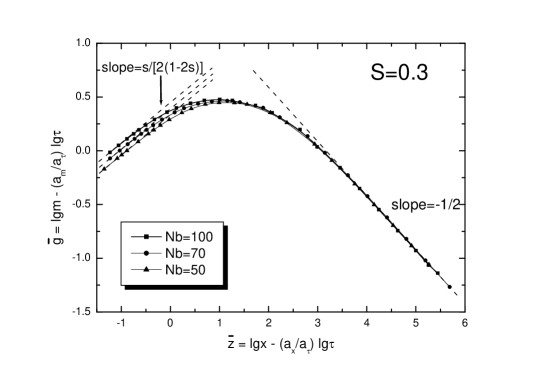
Figure 3: $\bar{g}=\text{lg}m-a_{m}/a_{\tau}\text{lg}\tau$ vs. $\bar{z}=\text{lg}x-a_{x}/a_{\tau}\text{lg}\tau$ for various $N_{b}$’s at $s=0.3,\Delta=0.1$ (squares with solid guiding lines). Here $a_{m}/a_{\tau}=1/2$ and $a_{x}/a_{\tau}=(1-2s)/s$ are used. From bottom to top, $N_{b}=50,70,100$, respectively. The dashed lines with slope $s/(2(1-2s))$ and $-1/2$ mark the large and small $\tau$ limit, respectively. As $N_{b}$ increases, the regime with almost zero slope expands.

The universal function $\bar{g}(\bar{z})$ is plotted in Fig.3 for $N_{b}\geq 50$. The downturn on the left part of the curve comes from the saturation of $m$ in the large $\tau$ regime. As $x$ gets smaller, the intermediate regime with zero slope extends, forming a pronounced plateau as described by Eq.(21). In the $m(\tau)$ curve, this corresponds to the extension of the regime with $\beta=1/2$ as $N_{b}$ increases.

The two-section behavior of $\bar{g}(\bar{z})$ in Eq.(21) agrees with Eq.(10). Putting Eq.(21) into Eq.(20), one gets $m(\tau,x)\propto x^{-1/2}\tau^{\beta_{NRG}}$ for $\tau\ll\tau_{cr}$ and $m(\tau,x)\propto\tau^{\beta_{MF}}$ for $\tau\gg\tau_{cr}$. The crossover $\tau_{cr}$ is determined by $z_{cr}^{0}=z_{cr}^{\theta}$ and $\bar{z}=\bar{x}-a_{x}/a_{\tau}\bar{\tau}$. We get $\tau_{cr}\propto x^{a_{\tau}/a_{x}}=x^{s/(1-2s)}$, same as in Eq.(11).

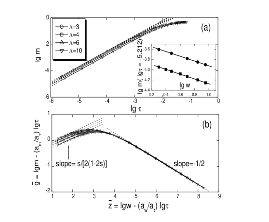
Figure 4: $\Lambda$ scaling behavior of the order parameter at $s=0.3,\Delta=0.1$. (a) $\text{lg}m(\epsilon=0)$ vs. $\text{lg}\tau$ for various $\Lambda$’s ($N_{b}=8,M_{s}=80$). Symbols with guiding lines are BNRG data and dashed lines are fitted lines. Inset: $\text{lg}m(\epsilon=0)$ at $\text{lg}\tau=-5.212$ as functions of $\text{lg}w$ for $N_{b}=8,M_{s}=80$ (squares) and $N_{b}=20,M_{s}=120$ (dots), respectively. The slopes of the fitting solid lines are $-0.46$. Other parameters are the same as in Fig.1. (b) Universal function of $\bar{g}=\text{lg}m-a_{m}/a_{\tau}\text{lg}\tau$ v.s. $\bar{z}=\text{lg}w-a_{w}/a_{\tau}\text{lg}\tau$ for different $\Lambda$’s. Here $a_{m}/a_{\tau}=1/2$ and $a_{w}/a_{\tau}=(1-2s)/s$ are used. The dashed lines with slope $s/(2(1-2s))$ and $-1/2$ mark the large and small $\tau$ limit, respectively. As $w$ decreases, the regime with almost zero slope expands.

Guided by the mean-field results Eq.(10), we also carry out scaling analysis for $m(\tau,w)$ with respect to $w=\Lambda-1$ (for $s=0.3$ and fixed $N_{b}$). In Fig.4(a), similar scaling behavior as in $m(\tau,x)$ is observed. In the inset, $\text{lg}m$ is plotted as a function of $\text{lg}w$ for a fixed $\text{lg}\tau$, giving a power law behavior with exponent $-0.46$, consistent with the $-1/2$ in Eq.(10) within numerical errors. By assuming that $m(\tau,w)$ is a GHF with scaling exponent $(a_{m},a_{\tau},a_{w})$, using the exponents Eq.(22), and by applying the data collapse procedure (not shown), we obtain $a_{m}/a_{\tau}=1/2$ and $a_{w}/a_{\tau}=(1-2s)/s=a_{x}/a_{\tau}$. In Fig.4(b), the universal function concerning $m(\tau,w)$ is plotted using the above exponents. Similar to Fig.3, the universal function has the form of Eq.(21), with $x\rightarrow w$. Fig.4 shows that the scaling variable $w$ plays a similar role as $x$. Therefore, the crossover scale $\tau_{cr}$ has an additional factor $w^{s/(1-2s)}$. For either $w=0$ or $x=0$, the $m(\tau,x,w)$ curve will have the classical exponent $\beta_{MF}$ in the regime $\tau\ll\tau_{sat}$. Here, again the NRG data agree with the mean-field expressions (10) and (11). The fact that $w$ becomes a scaling variable means the failure of the logarithmic discretization in NRG: $\Lambda$ may alter the universal quantities. This is solely due to the boson state truncation. As learned from the mean-field study, the parametrization scheme for the bath is relevant for the critical behavior once the bosons are no longer canonical.

Figure 5: (a) $\text{lg}m(\epsilon=0)$ vs. $\text{lg}\tau$ for different $\Delta$’s at $s=0.3$. From bottom to top, $\Delta=10^{-1},10^{-2},10^{-3},10^{-4},10^{-5}$, respectively. Symbols are BNRG data and the dashed lines are power law fit from small $\tau$ data, which agree with $\beta_{NRG}=(1-s)/(2s)$. Inset: $\text{lg}m$ at $\text{lg}\tau=-16$ as a function of $\Delta$ (symbols). The fitted line (solid line) has a slope $-0.821$ which agrees well with $-(1-s)^{2}/(2s)=-0.817$. (b)$\text{lg}\alpha_{c}$ as a function of $\text{lg}\Delta$. Symbols are BNRG data and the solid line is the fitted line with slope 0.703 which agrees with $1-s$. Calculated with $N_{b}=8$, $M_{s}=80$, and $\Lambda=4.0$.

As for $\Delta$, we show the BNRG results in Fig.5. The power law fits in Fig.5(a) and its inset disclose a double power behavior in the small $\tau$ limit: $m(\tau,\Delta)\propto\Delta^{\eta}\tau^{\beta_{NRG}}$. Here $\eta$ is an exponent to be determined below. In Fig.5(b), we show that BNRG produces $\alpha_{c}(1)\propto\Delta^{1-s}$, a result that has been established by BNRG and perturbative renormalization group study. Vojta1 To understand the exponent $\eta$, we resort to Eq.(10). If we collect the exponent of $\Delta$ in Eq.(10), and are careful enough to use the BNRG result $\alpha_{c}(1)=c(\Delta/\omega_{c})^{1-s}$ (instead of the mean-field one $\alpha_{c}(1)=\Delta s/(2\omega_{c})$) in Eq.(10), we get $\eta=-(1-s)^{2}/(2s)=-0.817$ for $s=0.3$. The exponent fitted from BNRG data is $-0.821$, as shown in the inset of Fig.5(a). The excellent agreement supports that the $\Delta$-dependence in BNRG results can also be summarized by Eq.(10). We checked other $s$ values in $0<s<1$ and confirmed this conclusion.

Combining the above results, we draw the conclusion that in the regime $0<s<1/2$, BNRG resutls for $m(\tau,\epsilon=0,\Delta,w,x)$ are well described by Eqs.(10), except that the $\Delta$-dependence of $\alpha_{c}(1)$ in the equation should be replaced by the BNRG form Eq.(18). Correspondingly, the crossover point $\tau_{cr}$ reads as

$$\tau_{cr}\propto\Delta^{1-s}(wx)^{s/(1-2s)}.$$ (38)

As a scaling variable, $\Delta$ is different from $w$ or $x$. As seen in Fig.5(a), when $\Delta$ decreases, both the $\beta_{NRG}$- and $\beta_{MF}$-exponent regimes in $m(\tau)$ curve shift to the left along the horizontal direction, but the $\beta_{MF}$-exponent regime does not expand. This is because another crossover scale $\tau_{sat}$, above which $m(\tau)\sim 1/2$, also decreases as $\Delta^{1-s}$. Indeed, using $m(\tau,\Delta)\propto[\tau/\alpha_{c}(1)]^{1/2}\propto(\tau/\Delta^{1-s})^{1/2}$ in $\tau_{cr}\ll\tau\ll\tau_{sat}$ and $m(\tau,\Delta)\sim 1/2$ in $\tau\gg\tau_{sat}$, one gets $\tau_{sat}\propto\Delta^{1-s}$, same as $\tau_{cr}$.

II.2.2 $m(\tau=0,\epsilon,\Delta,x,w)$

In this part, we fix $\tau=0$ and study the order parameter $m$ as a function of $\epsilon$. This is related to the exponent $\delta$.

Figure 6: $\text{lg}m(\tau=0)$ vs. $\text{lg}\epsilon$ for different $N_{b}$’s at $s=0.3,\Delta=0.1$. From bottom to top, $N_{b}=8,13,20,32,50,100$, respectively. Other parameters are $\Delta=0.1$, $\Lambda=10$, $M_{s}=80$. Symbols with solid guiding lines are BNRG data. The dashed line is power law fit for $N_{b}=100$ in small $\epsilon$ limit, which gives slope $1/\delta_{NRG}=0.533$ being consistent with $(1-s)/(1+s)$. The guiding dash-dotted line marks the asymptotic behavior $1/\delta=1/3$ in the large $N_{b}$ limit. Inset: $\text{lg}m(\tau=0)$ at $\epsilon=10^{-7}$ as functions of $\text{lg}x$ for $\Lambda=10,M_{s}=80$ (squares) and $\Lambda=4,M_{s}=120$ (dots), respectively. The dashed lines are guiding lines with slope $-s/(1+s)=-0.231$ to mark the power law behavior in large $N_{b}$ limit.

In Fig.6, $m(\epsilon,x)$ versus $\epsilon$ at $\tau=0$ is plotted for various $x$ values. Similar to $m(\tau,x)$, in the small-$\epsilon$ limit all curves for different $N_{b}$’s have the same power law $m(\epsilon,x)\propto\epsilon^{1/\delta_{NRG}}$ with $x$-dependent coefficients. For $s=0.3$, the fitted power $0.533$ agrees well with the mean-field expression $(1-s)/(1+s)=0.538$. For other $s$ values in $0<s<1/2$, the comparison is shown in Fig.14(b). The inset of Fig.6 supports $m(\epsilon,x)\propto x^{\theta^{\prime}}$ for fixed $\epsilon$ and large $N_{b}$, with the exponent $\theta^{\prime}$ to be determined below. Therefore, a double power form in the small $\epsilon$ limit is obtained, $m(\epsilon,x)\propto x^{\theta^{\prime}}\epsilon^{(1-s)/(1+s)}$. In the other limit where $\epsilon$ is much larger, the upper dashed line in Fig.6 marks out a finite regime where $m(\epsilon,x)\propto\epsilon^{1/\delta_{MF}}=\epsilon^{1/3}$. There is a crossover $\epsilon_{cr}\propto x^{-\theta^{\prime}/(1/\delta_{NRG}-1/\delta_{MF})}$ which separates the lower double-power regime from the upper classical regime. $\epsilon_{cr}$ goes to zero as $x\rightarrow 0$.

To obtain $\theta^{\prime}$, we carry out the scaling analysis based on GHF and do the data collapse in Fig.7. We assume that $m(\epsilon,x)$ is a GHF with scaling powers $(a_{m},a_{\epsilon},a_{x})$ and get $m(\epsilon,x)=\epsilon^{a_{m}/a_{\epsilon}}h(x/\epsilon^{a_{x}/a_{\epsilon}})$. The universal function $h(z)$ has a two-regime form similar to Eq.(21), i.e.,

$$\bar{h}(\bar{z})\propto\left\{\begin{array}[]{lll}const.,&(\bar{z}_{sat}\ll\bar{z}\ll\bar{z}_{cr});\\ &\\ \theta^{\prime}\bar{z},&(\bar{z}\gg\bar{z}_{cr}).\end{array}\right.$$ (42)

Here $\bar{z}=\bar{x}-(a_{x}/a_{\epsilon})\bar{\epsilon}$. Using $m(\epsilon,0)\propto\epsilon^{1/3}$ and $a_{m}/a_{x}=s/[2(1-2s)]$ confirmed before, we obtain

$$m(\epsilon,x)\propto\left\{\begin{array}[]{lll}x^{-s/(1+s)}\epsilon^{1/\delta_{NRG}},&(\epsilon\ll\epsilon_{cr});\\ &\\ \epsilon^{1/3}&(\epsilon\gg\epsilon_{cr}).\end{array}\right.$$ (46)

Here $\epsilon_{cr}\propto x^{a_{\epsilon}/a_{x}}$. This means $\theta^{\prime}=-s/(1+s)$ and

$$\frac{a_{m}}{a_{\epsilon}}=\frac{1}{3},\,\,\,\,\,$$

$$\frac{a_{x}}{a_{\epsilon}}=\frac{2(1-2s)}{3s}.$$ (47)

In the inset of Fig.6, the BNRG result for $\theta^{\prime}$ (symbols) compares favorably with the exponent $-s/(1+s)$ (dashed lines). In the inset of Fig.7, the exponents $a_{m}/a_{\epsilon}$ and $a_{x}/a_{\epsilon}$ extracted from ratios of the shifts $\delta m$, $\delta\epsilon$, and $\delta x$ agree well with Eq.(27) in the large $N_{b}$ limit, confirming Eq.(26). The similarity to the mean-field equation Eq.(14) is obvious. Using this $\theta^{\prime}$ we also obtain $\epsilon_{cr}\propto x^{3s/[2(1-2s)]}$. It agrees with the mean-field result in Eq.(15).

Figure 7: Data collapse of $\text{lg}m(\tau=0)$ vs. $\text{lg}\epsilon$ curves shown in Fig.6. The dashed straight line has a slope $(1-s)/(1+s)=0.538$. Inset: the ratio of the shift magnitudes $\delta\text{lg}x/\delta\text{lg}\epsilon$ (squares), and $\delta\text{lg}m/\delta\text{lg}\epsilon$ (dots) as functions of $N_{b}$. The dashed straight lines are $a_{x}/a_{\epsilon}=2(1-2s)/(3s)=0.889$ (upper) and $a_{m}/a_{\epsilon}=1/3$ (lower), respectively.

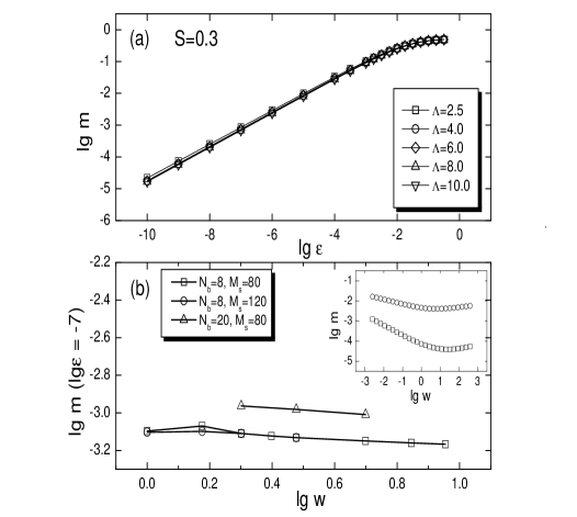
Figure 8: (a)$\text{lg}m(\tau=0)$ vs. $\text{lg}\epsilon$ for different $\Lambda$’s at $s=0.3$. (b)$\text{lg}m(\tau=0)$ vs. $\text{lg}w$ at $\epsilon=10^{-7}$ for various ($N_{b},M_{s}$)’s. The fitted slope is about $-0.07$ in the shown regime, different from $-s/(1+s)=-0.231$. This is probably due to the fact that $w$ is not small enough. Inset: the mean-field results $\text{lg}m$ vs. $\text{lg}w$ for $\tau=0,\epsilon=10^{-7}$ (cycles) and $\tau=10^{-7}$,$\epsilon=0$ (squares), respectively. Other parameters are $\Delta=0.1$, $N_{b}=8$.

The $\Lambda$ scaling analysis is carried out in Fig.8 for $m(\tau=0,\epsilon,w)$ for fixed $\Delta$, $N_{b}$ and $M_{s}$. In Fig.8(a), the small $\epsilon$ regime of the curves fulfills the power law $m(\epsilon,w)\propto\epsilon^{1/\delta_{NRG}}$ and the larger $\epsilon$ regime $m(\epsilon,w)\propto\epsilon^{1/\delta_{MF}}$. However, for a fixed $\epsilon$, the shift of the curve with $\Lambda$ is very weak for $\Lambda$ between $2.5$ and $10$. In Fig.8(b), the order parameter $m(\epsilon=10^{-7},w)$ does not fit a power law of $w$ as nicely as $m(\tau=\tau_{0},w)$ does in Fig.4. The data in the small $\Lambda$ regime are $M_{s}$ dependent. Here the crudest estimation from larger $\Lambda$ regime gives the power $-0.07$. Assuming a GHF form for $m(\epsilon,w)$ (at fixed $\tau=0$ and $x>0$) and using previously obtained relations among $a_{m},a_{\tau},a_{\epsilon}$ and $a_{w}$, we get

$$m(\epsilon,w)\propto\epsilon^{1/\delta_{NRG}}w^{-s/(1+s)},$$ (48)

same as in the mean-field result Eq.(14). The fitted power $-0.07$ is quite different from $-s/(1+s)=-0.231$.

We believe that this discrepancy is due to the fact that for $2\leqslant\Lambda\leqslant 10$, $w$ is not small enough to enter the scaling regime for observing the correct power law. This is in contrast to Fig.4 where a nice $w$-scaling persists up to $\Lambda=10$. We have not fully understood this contrast yet, but only mention that we observed similar differences in the mean-field calculations. There, the shift with $w$ is much more pronounced in $m(\tau=\tau_{0},\epsilon=0,w)$ than in $m(\tau=0,\epsilon=\epsilon_{0},w)$. The curves $\text{lg}m-\text{lg}w$ of the mean-field Hamiltonian are plotted in the inset of Fig.8(b), for $\tau=0$ (cycles) and $\epsilon=0$ (squares), respectively. It is seen that the expected power law behavior appears only when $\Lambda\ll 2$. In the regime $2<\Lambda<10$, the $\text{lg}m(\tau=0,\epsilon=\epsilon_{0},w)$ curve significantly deviates from the correct power law behavior, resembling the BNRG results. This supports our notion that much smaller $\Lambda$ is required to observe the $m(\tau=0,\epsilon=\epsilon_{0},w)\propto w^{-s/(1+s)}$ behavior. As a consequence of this reasoning, $w$ should also appear in the crossover scale $\epsilon_{cr}$ as a factor $w^{3s/(2(1-s))}$.

We checked our results for $N_{b}$ and $M_{s}$ up to $50$ and $300$, respectively, and found that the quality of the data is not improved. In the BNRG calculations, after each diagonalization, only the lowest $1/N_{b}$ fraction of eigen-states are kept. Hence, as $N_{b}$ increases, one needs larger $\Lambda$ or larger $M_{s}$ to compensate the error from discarding states. As a result, it is very difficult to produce reliable data in the large-$N_{b}$ and small-$\Lambda$ regimes. For a fixed $N_{b}$, it is known that to approach a smaller $\Lambda$ regime, one needs to use larger $M_{s}$. However, we did not find the expected power law behavior of $w$ up to $\Lambda=2$ using $N_{b}=8$ and $M_{s}=300$.

Figure 9: $\text{lg}m(\tau=0)$ vs. $\text{lg}\epsilon$ for different $\Delta$’s at $s=0.3$. From bottom to top, $\Delta=10^{-1},10^{-2},10^{-3},10^{-4}$, and $10^{-5}$, respectively. Symbols are BNRG data and dashed lines are power law fit, giving an average slope $0.539$ which agrees with $(1-s)/(1+s)=0.538$. Inset: $\text{lg}m(\tau=0)$ at $\text{lg}\epsilon=-11.292$ as a function of $\text{lg}\Delta$ (symbols). The fitting (solid line) gives a slope $-0.534$, being consistent with $\epsilon/\Delta$ scaling. Other parameters are $N_{b}=8$, and $M_{s}=80$.

In Fig.9, we study the $\Delta$ scaling in $m(\epsilon,\Delta)$ at $\tau=0$. The figure resembles that of $\text{lg}m(\tau,\Delta)-\text{lg}\Delta$. The double power form in the small $\epsilon$ regime is found to fulfill the $\epsilon/\Delta$ scaling, i.e.,

$$m(\epsilon,\Delta)\propto\left(\frac{\epsilon}{\Delta}\right)^{1/\delta_{NRG}},$$ (49)

with $1/\delta_{NRG}=(1-s)/(1+s)$. As $\Delta$ decreases, both $1/\delta_{MF}$- and $1/\delta_{NRG}$-exponent regimes move toward smaller $\epsilon$ along the horizontal direction. Simple analysis shows that a crossover scale $\epsilon_{sat}\propto\Delta$ separates the saturation regime $m\sim 1/2$ from the $1/\delta_{MF}$-exponent regime. $\epsilon_{cr}$ must have the same factor $\Delta$ because the classical exponent regime is not enlarged as $\Delta$ deceases. Summarizing these results, we get $\epsilon_{sat}>\epsilon_{cr}$ and

$$\epsilon_{cr}\propto(wx)^{\frac{3s}{2(1-2s)}}\Delta\,\,\,\,\,,$$

$$\epsilon_{sat}\propto\Delta\,\,\,\,\,.$$ (50)

These results concerning the scaling behavior with $\Delta$ is also consistent with the mean-field expression Eq.(14)-(15), provided that we use the BNRG result $\alpha_{c}(1)\propto\Delta^{1-s}$ in the equations.

II.2.3 Summary for $0<s<1/2$

We summarize the above analysis. Our main conclusion is that in the regime $0<s<1/2$, due to the boson state truncation, the order parameter $m$ produced by BNRG is a scaling function of variables $\tau$, $\epsilon$, $\Delta$, $x=1/N_{b}$, and $w=\Lambda-1$. Interestingly, this function agrees well with the mean-field equations for finite $N_{b}$, [Eqs.(10) and (11) and (14) and (15)], except that the $\Delta$-dependence of $\alpha_{c}(1)$ should be replaced by the corresponding BNRG one, i.e., $\alpha_{c}(1)\propto\Delta^{1-s}$. In the small-$\tau$ or -$\epsilon$ limits, the boson-state truncation $N_{b}$ introduces artificial exponents $\beta$ and $\delta$, which are different from the correct classical values. We summarize the BNRG results in $0<s<1/2$ as the following:

$$m(\tau,\epsilon=0,\Delta,x,w)$$ (56)

$$=\left\{\begin{array}[]{lll}c\left(\frac{\Delta}{\omega_{c}}\right)^{-\frac{(1-s)^{2}}{2s}}(wx)^{-\frac{1}{2}}\tau^{\frac{1-s}{2s}},&(\tau\ll\tau_{cr});\\ &\\ c^{\prime}\Delta^{-\frac{1-s}{2}}\tau^{\frac{1}{2}},&(\tau_{cr}\ll\tau\ll\tau_{sat});\\ &\\ 1/2,&(\tau\gg\tau_{sat}),\end{array}\right.$$

with the two crossover scales $\tau_{sat}>\tau_{cr}$ given by

$$\tau_{cr}\propto\Delta^{1-s}(wx)^{\frac{s}{1-2s}}\,\,\,\,\,,$$

$$\tau_{sat}\propto\Delta^{1-s}\,\,\,\,\,.$$ (58)

For $m(\tau=0,\epsilon,\Delta,x,w)$ we have

$$m(\tau=0,\epsilon,x,w)$$

$$=\left\{\begin{array}[]{lll}-c\Delta^{-\frac{1-s}{1+s}}(wx)^{-\frac{s}{1+s}}(\frac{\epsilon}{\omega_{c}})^{\frac{1-s}{1+s}},&(\epsilon\ll\epsilon_{cr});\\ &\\ -c^{\prime}(\frac{\epsilon}{\Delta})^{1/3},&(\epsilon_{cr}\ll\epsilon\ll\epsilon_{sat});\\ &\\ -1/2,&(\epsilon\gg\epsilon_{sat}).\end{array}\right.$$ (64)

with the two crossover scales $\epsilon_{sat}>\epsilon_{cr}$ given by

$$\epsilon_{cr}\propto(wx)^{\frac{3s}{2(1-2s)}}\Delta\,\,\,\,\,,$$

$$\epsilon_{sat}\propto\Delta\,\,\,\,\,.$$ (66)

For the role of $\Delta$ in the order parameter $m$, we observed $\tau/\Delta^{1-s}$ scaling in the function $m(\tau,\epsilon=0,\Delta,w,x)$, while the function $m(\tau=0,\epsilon,\Delta,w,x)$ has $\epsilon/\Delta$ scaling. These features are independent of the boson state truncation, and hence should hold also in the regime $1/2<s<1$. As we will see in the next section, this is indeed the case.

II.3 BNRG results for $s=0.7$

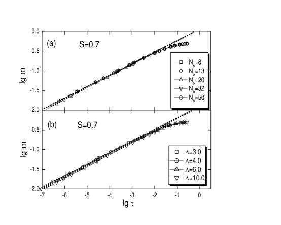
Figure 10: $\text{lg}m(\epsilon=0)$ vs. $\text{lg}\tau$ at $s=0.7$. (a) $\Lambda=10.0$ and $N_{b}=8,13,20,32,50$,respectively; (b) $N_{b}=8$ and $\Lambda=3.0,4.0,6.0,10.0$, respectively. Symbols are BNRG data and the dashed lines are power law fits. Other parameters are $\Delta=0.1$, and $M_{s}=80$.

In this section, to compare with the $0<s<1/2$ case, we study $s=0.7$, a generic value in the regime $1/2<s<1$. In this regime, the mean-field theory predicts classical exponents $\beta=1/2$ and $\delta=3$ for any $N_{b}$. The boson state truncation does not influence the Gaussian critical fixed point in the mean-field Hamiltonian.

For the full spin-boson model, BNRG predicts an interacting critical fixed point and nonclassical exponents $\beta$ and $\delta$. In Figs. 10(a) and 10(b), $\text{lg}m(\tau,\epsilon=0)-\text{lg}\tau$ curves are plotted for various $N_{b}$’s ($\Lambda=10$) and $\Lambda$’s ($N_{b}=8$), respectively. Other parameters are fixed. It is clearly seen that the situation is dramatically different from $s=0.3$: there is no $N_{b}$ or $\Lambda$ scaling. Therefore, the boson state truncation and $\Lambda$ do not influence the correct extraction of $\beta$.

Figure 11: $\text{lg}m(\epsilon=0)$ vs. $\text{lg}\tau$ at $s=0.7$ for different $\Delta$’s. From bottom to top, $\Delta=10^{-1},10^{-2},10^{-3},10^{-4},10^{-5}$, respectively. Symbols are BNRG data and the dashed lines are power law fit, giving an average slope 0.296. Inset on top left: $\text{lg}\alpha_{c}$ vs. $\text{lg}\Delta$ data gives the fitted slope 0.307, consistent with $1-s$. Inset on bottom right: $\text{lg}m$ at $\text{lg}\tau=-6.949$ as a function of $\text{lg}\Delta$ (symbols). The fitted slope is $-0.096$, close to $-\beta(1-s)=-0.089$, as expected from $\tau/\Delta^{1-s}$ scaling. Other parameters are $\Lambda=4.0$, $N_{b}=8$, $M_{s}=80$.

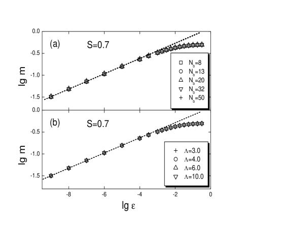
Figure 12: $\text{lg}m(\tau=0)$ vs. $\text{lg}\epsilon$ at $s=0.7$ for (a) different $N_{b}$’s and $\Lambda=10.0$, and (b) different $\Lambda$’s and $N_{b}=8$. Symbols are BNRG data and the dashed lines are power law fit, giving the average slopes $0.175$ and $0.173$ for (a) and (b), respectively. Other parameters are $\Delta=0.1$ and $M_{s}=80$.

In Fig.11, we study the $\Delta$ scaling at $s=0.7$ for $m(\tau,\epsilon=0)$. The main plot and the bottom right inset show that $m(\tau,\epsilon=0,\Delta)\propto\Delta^{\eta}\tau^{\beta}$. In the regime $1/2<s<1$, exact expression for $\beta$ as a function of $s$ is not known. If we assume that $m(\tau,\epsilon,\Delta)$ has $(\tau/\Delta^{1-s})$ scaling, as observed in the $s=0.3$ case, it is then easy to obtain

$$m(\tau,\epsilon=0,\Delta)\propto\Delta^{-(1-s)\beta}\tau^{\beta},\,\,\,\,\,\,(\tau\ll\tau_{sat}).$$ (67)

For $s=0.7$, the fitted value of $\eta$ is $-0.096$, which agrees with $-(1-s)\beta=-0.089$ quite well. We also checked other $s$ values in the regime $1/2<s<1$ and found good agreement, confirming the validity of $\tau/\Delta^{1-s}$ scaling in this case. The relation $\alpha_{c}(1)\propto\Delta^{1-s}$ is demonstrated in the top left inset of Fig. 11. $\tau_{sat}\propto\Delta^{1-s}$ is the crossover scale separating the power-law regime from the saturation regime $m\sim 1/2$.

Similar analysis is carried out for $m(\tau=0,\epsilon,\Delta,x,w)$. In Figs. 12(a) and 12(b), we plot this function for $s=0.7$ and $\Delta=0.1$, for various $N_{b}$’s ($\Lambda=10$) and $\Lambda$’s ($N_{b}=8$). No $N_{b}$ or $\Lambda$ scaling is observed, similar to the curves $m(\tau,\epsilon=0,\Delta,x,w)$ shown in Fig.10.

The $\Delta$ scaling carried out in Fig.13 shows that the exponent $\delta$ fulfills the expression $(1+s)/(1-s)$, even in the $1/2<s<1$ regime. This is consistent with the previous findings of the hyperscaling relation $\delta=(1+x)/(1-x)$ and $x=s$. Vojta1 In the inset of Fig.13, $\text{lg}m-\text{lg}\Delta$ is shown for fixed $\epsilon$, disclosing a power law behavior consistent with $m(\tau=0,\epsilon,\Delta)\propto\Delta^{-(1-s)/(1+s)}$. This implies the $\epsilon/\Delta$ scaling in the regime $1/2<s<1$. Therefore, we have

$$m(\tau=0,\epsilon,\Delta,w,w)\propto\left(\frac{\epsilon}{\Delta}\right)^{\frac{1-s}{1+s}}\,\,\,\,\,(\epsilon\ll\epsilon_{sat}).$$ (68)

Here $\epsilon_{sat}\propto\Delta$ is the crossover scale separating the power law regime from the saturation regime $m\sim 1/2$.

Figure 13: $\text{lg}m(\tau=0)$ vs. $\text{lg}\epsilon$ at $s=0.7$ for different $\Delta$’s. Symbols are BNRG data and dashed lines are power law fit. From bottom to top, $\Delta=10^{-1},10^{-2},10^{-3},10^{-4},10^{-5}$, respectively. Inset: $\text{lg}m(\tau=0)$ at $\text{lg}\epsilon=-10.423$ as a function of $\text{lg}\Delta$. The solid line is a power law fit in small $\Delta$ limit and the slope $-0.179$ is close to $-(1-s)/(1+s)=-0.177$, as expected from $\epsilon/\Delta$ scaling. Other parameters are $\Lambda=4.0$, $N_{b}=8$, and $M_{s}=80$.

II.4 $s=0$ and $s=1/2$

The boundary cases $s=0$ and $s=1/2$ need some discussions. For $s=0$, the mean-field solution at finite $N_{b}$ gives [Eq.(12)] $m(\tau,\epsilon=0)\propto\text{exp}(-\Delta/4\omega_{c}\tau)$ and the crossover scale $\tau_{cr}$ becomes independent of $wx$. This means that $\tau_{cr}$ is large and decreases with $wx$ at subleading order. We carried out the BNRG calculation for $s=0$ with $10^{-6}\leqslant\Delta\leqslant 10^{-2}$ and $10\leqslant N_{b}\leqslant 50$. Using the exponential fit, we obtain $\alpha_{c}=0$ within an error less than $10^{-7}$. For a fixed $N_{b}$, $m(\tau,\epsilon=0)$ shows a nice exponential behavior $m\propto\text{exp}(-c/\tau)$ with $c\approx(0.27\pm 0.02)\Delta$. This is consistent with the mean-field expression (12). For the prefactor, we observe the $x^{-1/2}$ behavior using $8<N_{b}\leqslant 50$, and find the $-1/2$ exponent of $w$ using $\Lambda<2.5$ and $M_{s}>200$. However, we also find a perfect $\tau/\Delta$ scaling at $s=0$, being different from Eq. (12). By combining these results, we expect the crossover scale $\tau_{cr}\propto-\Delta/\text{ln}(wx)$. As for $m(\tau=0,\epsilon)$, BNRG gives the exact result $m(\tau=0,\epsilon)=-\epsilon/(2\Delta)$ since at $\tau=\alpha=0$ the spin is decoupled from the bath.

For $s=1/2$, contrary to $s=0$, the powers of $wx$ in the expressions for $\tau_{cr}$ and $\epsilon_{cr}$ diverge, leading to the vanishing of the latter for $wx<1$. Therefore, the classical regimes in $m(\tau,\epsilon=0)$ and $m(\tau=0,\epsilon)$ expand to the zero $\tau$ or $\epsilon$ limit, even for finite $N_{b}$’s and $\Lambda>1$. Indeed, using $N_{b}=8$ and $\Lambda=4$, BNRG gives accurate $\beta_{MF}$ and $\delta_{MF}$ at $s=1/2$, as shown in Fig.14(a) and (b), respectively. For $s=1/2$, corrections to power laws in $m(\tau,\epsilon=0)$ and $m(\tau=0,\epsilon)$ may arise in the subleading order in which $x$ and $w$ may play some roles. However, such effects are difficult to observe in the BNRG data because of numerical errors and fitting errors.

III Summary and Discussion

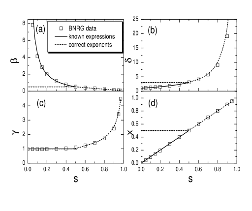
Figure 14: Critical exponents of the spin-boson model as functions of $s$: (a) $\beta$, (b) $\delta$, (c) $\gamma$, and (d) $x$. The squares are the exponents fitted from BNRG data with finite $N_{b}$. The solid lines are $\beta_{NRG}=(1-s)/(2s)$, $\delta_{NRG}=(1+s)/(1-s)$, $\gamma_{NRG}=1$, and $x_{NRG}=s$, respectively. The dashed lines are the correct exponents free from boson state truncation error and the mass flow error.

In Fig.14, we summarize the exponents $\beta$, $\delta$, $\gamma$ and $x$ for the spin-boson model in the whole regime $0<s<1$. The squares in the figure show the naive BNRG results obtained using finite $N_{b}$. The solid lines for $\beta$ and $\delta$ in the regime $0<s<1/2$, as shown in Fig.14(a) and (b), are $\beta=2s/(1-s)$ and $\delta=(1+s)/(1-s)$, the exact solution of the mean-field Hamiltonian with finite $N_{b}$. They agree well with the BNRG data (squares). The dashed lines are the correct values extracted from the scaling analysis. They deviate significantly from the BNRG results in $0\leqslant s<1/2$. In the regime $1/2\leqslant s<1$, the boson state truncation error and mass flow error still exist but they do not influence the exponents.

We also studied the magnetic susceptibility $\chi$ using BNRG in the regime $0\leqslant s\leqslant 1/2$ (squares in Fig.14(c)). It is found that $\chi(\tau,T=0)$ curve is independent of $w$ and $x$ and $\gamma=1$ holds at high precision. For the $\Delta$ dependence, BNRG calculations for various $s$ in the regime $0\leqslant s<1$ confirm the scaling form $\chi\propto\Delta^{-1}(\tau/\Delta^{1-s})^{-1}$, being consistent with $m(\tau,\epsilon,\Delta)=f(\tau/\Delta^{1-s},\epsilon/\Delta)$. In the mean-field theory, the factors containing $wx$ cancel each other and one obtains $\chi\propto\Delta^{-1}(\tau/\alpha_{c}(1))^{-1}$, independent of $wx$. It covers the BNRG result when $\alpha_{c}(1)$ is replaced by $\Delta^{1-s}$. In the regime $1/2<s<1$, the BNRG result for $\gamma$ follows a nonclassical curve [squares and the dashed line in Fig. 14(c)], the exact expression of which is not known yet. It is related to $\beta$ and $\delta$ through hyperscaling relations.

The temperature dependence $\chi(T)$ at $\tau=0$ is governed by the exponent $x$. We did not find any observable shift in $\chi(\tau=0,T)$ with the changing of $N_{b}$ or $\Lambda$ in the range $8<N_{b}<20$ and $2<\Lambda<10$. We always obtain $x=s$ in the regime $0<s<1/2$. This indicates that the mass-flow problem is deeply rooted in the NRG algorithm and can not be solved by the scaling method that we discuss in this paper. According to the analysis of the mass-flow problem in NRG,  Vojta2 ; Vojta3 $x=1/2$ should hold in the regime $0\leqslant s\leqslant 1/2$ and $x=s$ in $1/2<s<1$. This conclusion together with the BNRG result are summarized in Fig. 14(d) for completeness.

To conclude, we confirm the statements in Ref. Vojta2, that for the spin-boson model, the critical exponents $\beta$ and $\delta$ are classical in the regime $0\leqslant s\leqslant 1/2$, while are nonclassical in $1/2<s<1$. BNRG with finite $N_{b}$ produces artificial interacting critical fixed point in the regime $0\leqslant s<1/2$, and the extracted $\beta$ and $\delta$ are incorrect. In the regime $1/2\leqslant s<1$, boson-state truncation does not play a role and BNRG results are correct. Scaling analysis with respect to $x=1/N_{b}$ and $w=\Lambda-1$ can be used as a supplement to ordinary BNRG to overcome the boson-state truncation error. It is also observed that the order parameter has the scaling form $m(\tau,\epsilon,\Delta)=f(\tau/\Delta^{1-s},\epsilon/\Delta)$ in the whole regime $0\leqslant s<1$.

Two features of the BNRG results can be understood in terms of the mean-field Hamiltonian. First, as shown in Eqs. (31) and (33), the boson-state truncation error disappears in the limit $\Lambda=1$. Second, the truncation $N_{b}$ influences only the exponents but not the critical coupling $\alpha_{c}$. In the mean-field Hamiltonian [Eqs. (6)-(8)], the $n$th boson mode has a displacement $\gamma_{n}/\xi_{n}$ and its coupling strength to the spin is proportional to $\gamma_{n}$. Both $\gamma_{n}$ and $\xi_{n}$ decay exponentially with increasing $n$, but the ratio $\gamma_{n}/\xi_{n}$ diverges as $\Lambda^{(1-s)n/2}$. The low-energy modes (with large $n$) are more displaced and need more states to describe. Therefore, truncation of the state influences mostly the low-energy modes and not the high-energy modes. In the limit $\Lambda=1$, however, there is no divergence in the displacement and all the modes can be described equally well by a finite $N_{b}$, hence the truncation error disappears. Since the critical exponents are closely related to the energy distribution and the displacement behavior of the low-energy boson modes, they are susceptible to the truncation. While the critical coupling is dominated by the integral properties of the spectrum in which the high-energy modes have more weights, it is thus only very weakly influenced by the truncation.

Our results support the validity of quantum-to-classical mapping for the spin-boson model in the regime $0\leqslant s<1/2$. Note that our picture of $m(\tau)$ for the truncated spin-boson model is consistent with the results of exact diagonalization study in Ref. Alvermann1, . There, although a different basis set is used, in principle, the boson-state truncation error also exists and the nonclassical exponents should be present in the low-energy limit. However, the fitting of data relatively far away from the critical point (note the linear scale in Fig. 3 of Ref. Alvermann1, ) coincidentally misses the nonclassical regime and produces the correct classical exponent $\beta_{MF}$.

For other quantum impurity models such as the Bose-Fermi-Kondo model (BFKM) model Si1 ; Zhu1 ; Zhu2 and its anisotropic version, the Ising-BFKM, Glossop1 similar quantum-to-classical mapping arguments supports Gaussian fixed points in the regime $0\leqslant s<1/2$. Correspondingly, one expects $\beta=1/2$, $\delta=3$ and $x=1/2$. Neither hyperscaling relations nor $\omega/T$ scaling should hold. However, variouls studies using BNRG Glossop1 , QMC simulation Kirchner2 ; Kirchner3 ; Kirchner4 , $\epsilon$-expansion Zhu1 ; Si2 and the large-N limit analysis Si1 ; Zhu2 ; Burdin1 all point to the failure of the quantum-to-classical mapping in these systems: they obtained interacting fixed point and nonclassical exponents. Especially, for the anisotropic BFKM with a sub-Ohmic boson bath, the exponents are found to be the same as $\beta_{NRG}$ and $\delta_{NRG}$ of the spin-boson model.

In light of the present study, it is possible that the same boson state truncation error may exist in the BNRG study of the Ising BFKM in Ref. Glossop1, and lead to incorrect $\beta$ and $\delta$ in the regime $0<s<1/2$. Note that the boson state truncation problem cannot be remedied by going to smaller energy scales. Glossop1 ; Kirchner4 Since the fermion bath in the Ising BFKM can be integrated out to produce an additional boson bath with Ohmic spectrum, the critical behavior should be dominated by the sub-Ohmic one, leading to the expectation that it belongs to the same universality class as the spin-boson model. In the quantum Monte Carlo simulations, it was observed that the truncation of correlations in the imaginary time axis is the key to produce the interacting critical point. Kirchner4 Otherwise Gaussian behavior will obtain. These may be signatures that the quantum-to-classical mapping holds also for the Ising BFKM in $0\leqslant s<1/2$. It is straightforward to examine this statement using BNRG supplemented with the $N_{b}$ scaling.

As far as the isotropic BFKM is concerned, the situation seems different. Here, the symmetry is different from the spin-boson model and the Berry phase effect is claimed to be nontrivial. Kirchner5 Much work has been done for this model, supporting the failure of the quantum-to-classical mapping in the sub-Ohmic regime. Zhu2 ; Kirchner3 ; Kirchner5 Due to the very subtle nature of this problem, however, exact numerical studies are still desirable as a further confirmation. Both the isotropic and the anisotropic BFKM are at the core of studying the Kondo lattice with Ruderman-Kittel-Kasuya-Yoshida (RKKY) interactions using the extended dynamical mean-field theory. Si1 ; Si2 ; Glossop2 ; Zhu3 ; Zarand1 ; Zhu4 ; Grempel1 Therefore, any definite conclusions concerning these impurity models will have important impact on the understanding of the competition between Kondo screening and the antiferromagnetic state in the heavy-fermions metals. Si1 ; Gegenwart1

In summary, we carried out systematic BNRG studies for the spin-boson model in the sub-Ohmic regime, supplemented with the scaling analysis for the boson state truncation $x=1/N_{b}$ and the logarithmic discretization parameter $w=\Lambda-1$. For $0<s<1/2$, the function $m(\tau,\epsilon=0,\Delta,x,w)$ [$m(\tau=0,\epsilon,\Delta,x,w)$] is shown to bear a multiple power form in the small-$\tau$ (-$\epsilon$) limit. Classical exponent $\beta=1/2$ ($\delta=3$) is identified in the regime $\tau\gg\tau_{cr}$ ($\epsilon\gg\epsilon_{cr}$), agreeing with the conclusion from the quantum-to-classical mapping. The crossover scale $\tau_{cr}$ ($\epsilon_{cr}$) goes to zero in the small $x$ or $w$ limits in a power law. This presents a scenario of how the boson-state truncation error disappears in the limit $N_{b}\rightarrow\infty$. The observation that $x$ and $w$ always appear as a product $(wx)$ indicates that, in the regime $0\leqslant s<1/2$, the boson-state truncation invalidates the logarithmic discretization scheme, which is the basis of NRG. Independent of the issue of boson-state truncation, we also find that the scaling form for the order parameter $m(\tau,\epsilon,\Delta)=f(\tau/\Delta^{1-s},\epsilon/\Delta)$ in the whole regime $0\leqslant s<1$.

IV Acknowledgments

The authors acknowledge helpful discussions with Ralf Bulla, Hsiu-Hau Lin, and Matthias Vojta. This work is supported by the 973 Program of China under Grant No. 2007CB925004 and by National Natural Science Foundation of China under Grant No.11074302.

Appendix A Critical Exponents of the Mean-Field Spin-Boson Model

In this appendix, we present the calculation of the critical exponents $\beta$, $\delta$, and $\gamma$ for the mean-field spin-boson Hamiltonian.

The Hamiltonian of the spin-boson model reads as

$$H_{sb}=-\frac{\Delta}{2}\sigma_{x}+\frac{\epsilon}{2}\sigma_{z}+\frac{1}{2}\sigma_{z}\sum_{i}\lambda_{i}\left(a_{i}+a_{i}^{\dagger}\right)+\sum_{i}\omega_{i}a_{i}^{\dagger}a_{i}.$$ (69)

The mean-field Hamiltonian is (neglecting a constant)

$$H_{mf}= -\frac{\Delta}{2}\sigma_{x}+\left[\frac{\epsilon}{2}+\frac{1}{2}\sum_{i}\lambda_{i}\langle a_{i}+a_{i}^{{\dagger}}\rangle\right]\sigma_{z}$$ (70)

$$+\sum_{i}\omega_{i}a_{i}^{{\dagger}}a_{i}+\frac{\langle\sigma_{z}\rangle}{2}\sum_{i}\lambda_{i}\left(a_{i}+a_{i}^{{\dagger}}\right).$$

For a finite $N_{b}$, the critical behavior depends severely on the parameterization scheme for $\{\omega_{i},\lambda_{i}\}$ as well as on the discretization scheme. In order to compare the exponents with the NRG ones, we carry out the logarithmic discretization as in NRG and get

$$H_{mf}^{LD}= -\frac{\Delta}{2}\sigma_{x}+\left[\frac{\epsilon}{2}+\frac{1}{2\sqrt{\pi}}\sum_{n=0}^{\infty}\gamma_{n}\langle a_{n}+a_{n}^{{\dagger}}\rangle\right]\sigma_{z}$$ (71)

$$+\sum_{n=0}^{\infty}\xi_{n}a_{n}^{{\dagger}}a_{n}+\frac{\langle\sigma_{z}\rangle}{2\sqrt{\pi}}\sum_{n=0}^{\infty}\gamma_{n}\left(a_{n}^{\dagger}+a_{n}\right),$$

where the superscript LD denotes the logarithmic discretization. $\gamma_{n}$ and $\xi_{n}$ are obtained from standard procedure Bulla1 ; Bulla3 and given in Eq.(7) and (8) in the main text. In Eq.(A3), the spin and boson degrees of freedom decouple and we get $H_{mf}^{LD}=H_{spin}+H_{boson}$, where

$$H_{spin}=-\frac{\Delta}{2}\sigma_{x}+\frac{1}{2}(\epsilon+d)\sigma_{z},$$ (72)

and

$$H_{boson}=\sum_{n=0}^{\infty}\xi_{n}a_{n}^{{\dagger}}a_{n}+\frac{1}{2}\langle\sigma_{z}\rangle\sum_{n=0}^{\infty}\frac{\gamma_{n}}{\sqrt{\pi}}\left(a_{n}^{\dagger}+a_{n}\right).$$ (73)

Here

$$d=\sum_{n=0}^{\infty}\frac{\gamma_{n}}{\sqrt{\pi}}\langle a_{n}^{\dagger}+a_{n}\rangle.$$ (74)

For $N_{b}=\infty$, $H_{boson}$ can be solved exactly. For finite $N_{b}$, it is no longer exactly solvable. In Ref. Hou1, , $H_{mf}^{LD}$ is solved numerically and the critical behavior is studied. Here, we start from the single mode Hamiltonian

$$H=a^{\dagger}a+\theta(a^{\dagger}+a).$$ (75)

In the small $\theta$ limit, the ground state is not influenced by the truncation and we have $\langle a^{\dagger}+a\rangle_{G}=-2\theta$ and $\langle a^{\dagger}a\rangle_{G}=\theta^{2}$. In the large $\theta$ limit, the number of bosons in the ground state is confined by the boson state truncation $N_{b}$. Therefore in this limit $\langle a^{\dagger}a\rangle_{G}=N_{b}$. For the displaced harmonic oscillator, to leading order of $N_{b}$ we have $\langle a+a^{\dagger}\rangle_{G}=-2\sqrt{\langle a^{\dagger}a\rangle_{G}}=-2\sqrt{N_{b}}$. The crossover scale is determined by equating the two situations. In summary, we have

$$\langle a^{\dagger}+a\rangle_{G}=\left\{\begin{array}[]{lll}-2\theta,&(\theta\ll\sqrt{N_{b}});\\ &\\ -2\sqrt{N_{b}},&(\theta\gg\sqrt{N_{b}}).\end{array}\right.$$ (79)

We confirmed this result numerically. Here $\langle...\rangle_{G}$ denotes the ground state average. $\langle a_{n}^{\dagger}+a_{n}\rangle_{G}$ has different form in the regimes $n\ll n_{0}$ and $n\gg n_{0}$. Here $n_{0}$ separates the freely biased mode (small $n$) from the saturated biased mode (large $n$). We can then solve $H_{boson}$ approximately and obtain one of the mean-field equations from Eq.(A6),

$$d\approx-\frac{1}{\pi}\langle\sigma_{z}\rangle\sum_{n=0}^{n_{0}}\frac{\gamma_{n}^{2}}{\xi_{n}}-2\sqrt{\frac{N_{b}}{\pi}}\sum_{n=n_{0}+1}^{\infty}\gamma_{n},$$ (80)

with $n_{0}$ determined by equating $\sqrt{N_{b}}$ with the effective bias,

$$\frac{1}{2}\langle\sigma_{z}\rangle\frac{\gamma_{n_{0}}}{\sqrt{\pi}\xi_{n_{0}}}=\sqrt{N_{b}}.$$ (81)

Introducing $x=1/N_{b}$ and $m=\langle\sigma_{z}\rangle/2$ and summing over $n$ in Eq.(A9) produces

$$d=a_{1}(\Lambda)\alpha m+\left[a_{2}(\Lambda)+b_{1}(\Lambda)\right]\alpha^{\frac{1}{1-s}}x^{\frac{s}{1-s}}m^{\frac{1+s}{1-s}}.$$ (82)

The parameters $a_{1}(\Lambda)$, $a_{2}(\Lambda)$, and $b_{1}(\Lambda)$ read

$$a_{1}(\Lambda)=-\frac{4(2+s)}{(1+s)^{2}}\frac{\left[1-\Lambda^{-(1+s)}\right]^{2}}{\left[1-\Lambda^{-s}\right]\left[1-\Lambda^{-(2+s)}\right]}\omega_{c},$$ (83)

$$a_{2}(\Lambda) = 2^{\frac{2-s}{1-s}}(1+s)^{-\frac{2+s}{1-s}}(2+s)^{\frac{1+s}{1-s}}\left[1-\Lambda^{-(2+s)}\right]^{-\frac{1+s}{1-s}}$$ (84)

$$\left[1-\Lambda^{-(1+s)}\right]^{\frac{2+s}{1-s}}\frac{1}{\Lambda^{s}-1}\omega_{c},$$

and

$$b_{1}(\Lambda)=-a_{2}(\Lambda)\frac{\Lambda^{s}-1}{\Lambda^{(1+s)/2}-1}.$$ (85)

The other mean-field equation from solving $H_{spin}$ is

$$m=\frac{1}{2}\frac{\Delta^{2}-\left[\epsilon+d+\sqrt{\Delta^{2}+(\epsilon+d)^{2}}\right]^{2}}{\Delta^{2}+\left[\epsilon+d+\sqrt{\Delta^{2}+(\epsilon+d)^{2}}\right]^{2}}.$$ (86)

Near the critical point, it reduces to

$$m=-\frac{\epsilon+d}{2\Delta}+\frac{1}{4}\left(\frac{\epsilon+d}{\Delta}\right)^{3}+O\left(\frac{\epsilon+d}{\Delta}\right)^{4}.$$ (87)

Putting Eq.A(11) into the above equation and keeping only the leading term of each type, one gets

$$m= -\frac{\epsilon}{2\Delta}-\frac{a_{1}(\Lambda)\alpha m}{2\Delta}+\frac{1}{4\Delta^{3}}\left[a_{1}(\Lambda)\alpha m\right]^{3}$$ (88)

$$-\frac{a_{2}(\Lambda)+b_{1}(\Lambda)}{2\Delta}\alpha^{\frac{1}{1-s}}x^{\frac{s}{1-s}}m^{\frac{1+s}{1-s}}.$$

From this equation the critical coupling strength is obtained as $\alpha_{c}(\Lambda)=-2\Delta/a_{1}(\Lambda)$. It is remarkable that it is independent of the boson state truncation $N_{b}$. Introducing $\tau=\alpha-\alpha_{c}(\Lambda)$ to measure the distance to the critical point, we get the self-consistent equation as

$$-\frac{\epsilon}{\Delta}-\frac{a_{2}(\Lambda)+b_{1}(\Lambda)}{\Delta}\left[\alpha_{c}(\Lambda)\right]^{\frac{1}{1-s}}x^{\frac{s}{1-s}}m^{\frac{1+s}{1-s}}$$

$$+\frac{2\tau}{\alpha_{c}(\Lambda)}m-4m^{3}=0.$$ (89)

To investigate the role of $\Lambda$, we define $w=\Lambda-1$ and expand $\alpha_{c}(\Lambda)$, $a_{2}(\Lambda)$ and $b_{1}(\Lambda)$ to leading order of $w$. Finally we get the self-consistent equation in terms of $\tau$, $\epsilon$, $\Delta$, $w$, and $x$ as (keeping $\alpha_{c}(\Lambda)$ in the definition of $\tau$ unchanged)

$$\frac{2\tau}{\alpha_{c}(1)}m-4m^{3}-\frac{\epsilon}{\Delta}-c\frac{\omega_{c}}{\Delta}\left[\alpha_{c}(1)\right]^{\frac{1}{1-s}}(wx)^{\frac{s}{1-s}}m^{\frac{1+s}{1-s}}=0.$$ (90)

Here $\alpha_{c}(1)=\Delta s/(2\omega_{c})$ is the critical $\alpha$ value for $\Lambda=1$. $c=2^{(2-s)/(1-s)}\left[1/s-2/(1+s)\right]$ is a constant. It is noted here that the anomalous term involving the $(wx)^{s/(1-s)}$ comes solely from the factor $a_{2}(\Lambda)+b_{1}(\Lambda)$, instead of from expansions of $\alpha_{c}(\Lambda)$ in Eq.(A18). Solving this equation in various limits produces the analytical expressions Eqs.(9)-(16).

Eq.(A19) reduces to standard mean-field equation and gives $\beta=1/2$, $\delta=3$, when the $m^{3}$ term dominates over the anomalous term $(wx)^{s/(1-s)}m^{(1+s)/(1-s)}$. This is the case when $m$ is small in the regime $1/2<s<1$, or when $wx\ll m$ in the regime $0<s<1/2$. The anomalous term will dominate over the $m^{3}$ term and give $\beta=(1-s)/(2s)$ and $\delta=(1+s)/(1-s)$, when $m\rightarrow 0$ in the regime $0<s<1/2$. Considering different regimes of $\tau$ and $\epsilon$, we get the expressions (9) and (10) and (13) and (14). The crossover scales $\tau_{cr}$ [Eq. (11)] and $\epsilon_{cr}$ [Eq.(15)] are obtained by equating the expressions in the classical and nonclassical regimes.

At $s=0$, Eq. A(10) is replaced with

$$n_{0}=\frac{1}{\text{ln}\Lambda}\text{ln}\left[\frac{(1+\Lambda^{-1})^{2}}{1-\Lambda^{-1}}\frac{1}{8\alpha xm^{2}}\right].$$ (91)

The summation in Eq.A(9) produces

$$d= -8\alpha m\omega_{c}\frac{1-\Lambda^{-1}}{(1+\Lambda^{-1})\text{ln}\Lambda}\text{ln}\left[\frac{\Lambda(1+\Lambda^{-1})^{2}}{8(1-\Lambda^{-1})x\alpha m^{2}}\right]$$ (92)

$$-8\alpha m\omega_{c}\frac{\Lambda^{-1/2}+\Lambda^{-1}}{1+\Lambda^{-1}}.$$

This gives $\alpha_{c}=0$. Expanding $d$ at $\Lambda=1$ to leading order and combining Eq.(A16), we get the order parameter for $s=0$,

$$m(\tau,\epsilon=0,\Delta,x,w)=c\frac{1}{2}(wx\tau)^{-\frac{1}{2}}e^{-\frac{\Delta}{4\omega_{c}\tau}},$$ (93)

and

$$m(\tau=0,\epsilon,\Delta,x,w)=-\frac{\epsilon}{2\Delta}.$$ (94)

Here, $c$ is a constant independent of $\Delta$, $x$, and $w$. Note that if one takes the $x\rightarrow 0$ limit first and then takes the limit $s\rightarrow 0$, Eq.(A22) becomes

$$m(\tau,\epsilon=0,\Delta,x=0,w)=\left\{\begin{array}[]{lll}1/2,&(\tau>0);\\ &\\ 0,&(\tau=0).\end{array}\right.$$ (98)

The magnetic susceptibility $\chi$ can be obtained by taking derivative on both sides of Eq. (A19) with respect to $\epsilon$. This leads to the expression

$$-\Delta\chi=$$

$$\left[\frac{c(1+s)}{1-s}\frac{\omega_{c}}{\Delta}\left[\alpha_{c}(1)\right]^{\frac{1}{1-s}}(wx)^{\frac{s}{1-s}}m^{\frac{2s}{1-s}}+12m^{2}-\frac{2\tau}{\alpha_{c}(1)}\right]^{-1}.$$

Here, $c=2^{(2-s)/(1-s)}\left[1/s-2/(1+s)\right]$. Analyzing this equation in different $\tau$ regimes, we obtain $\chi(\tau,\Delta)=-\alpha_{c}(1)/(4\Delta\tau)$ in the regime $1/2\leqslant s<1$, and

$$\chi(\tau,\Delta)=\left\{\begin{array}[]{lll}-\frac{\alpha_{c}(1)}{4\Delta\tau}&(\tau\gg\tau_{cr}),\\ &\\ -\frac{1-s}{4s}\frac{\alpha_{c}(1)}{\Delta\tau}&(\tau\ll\tau_{cr}).\end{array}\right.$$ (103)

in the regime $0\leqslant s<1/2$. This gives the exponent $\gamma=1$, independent of $N_{b}$ and $w$.

We also studied the critical behavior of $m(\tau,\epsilon,\Delta,x)$ using other parametrization and discretization schemes for the bath spectrum. It is found that for finite $N_{b}$, the critical exponents $\beta$ and $\delta$ are strongly dependent on the scheme. For $N_{b}=\infty$, they all reduce to the mean-field values.

References

- (1) U. Weiss, Quantum Dissipative Systems (World Scientific, Singapore, 1999), 2nd edition.
- (2) A. J. Leggett et al., Rev. Mod. Phys. 59, 1 (1987).
- (3) H. Spohn and R. Dümcke, J. Stat. Phys. 41, 389 (1985); S. Kehrein and A. Mielke, Phys. Lett. A 219, 313 (1996).
- (4) R. Bulla, N.-H. Tong, and M. Vojta, Phys. Rev. Lett. 91, 170601 (2003); R. Bulla, H.-J. Lee, N.-H. Tong, and M. Vojta, Phys. Rev. B 71, 045122 (2005).
- (5) M. Vojta, N. H. Tong, and R. Bulla, Phys. Rev. Lett. 94, 070604 (2005).
- (6) N.-H. Tong and M. Vojta, Phys. Rev. Lett. 97, 016802 (2006).
- (7) For reviews, see R. Bulla, T. A. Costi, and T. Pruschke, Rev. Mod. Phys. 80, 395 (2008); M. Vojta, Phil. Mag. 86, 1807 (2006).
- (8) K. G. Wilson, Rev. Mod. Phys. 47, 773 (1975).
- (9) H.-J. Lee and R. Bulla, Euro. Phys. J. B 56, 199 (2007); H.-J. Lee, K. Byczuk, and R. Bulla, Phys. Rev. B 82, 054516 (2010).
- (10) S. Tornow, N.-H. Tong, and R. Bulla, Europhys. Lett. 73, 913 (2006); S. Tornow, N.-H. Tong, and R. Bulla, J. Phys. Condens. Matter, 18, 5985 (2006); R. Bulla, S. Tornow, and F. B. Anders, Adv. Sol. Stat. Phys. 47, 69 (2008); S. Tornow, R. Bulla, F. B. Anders, and A. Nitzan, Phys. Rev. B 78, 035434 (2008).
- (11) F. J. Dyson, Commun. Math. Phys.12, 91 (1969).
- (12) M. E. Fisher, S.-K. Ma, and B. G. Nickel, Phys. Rev. Lett. 29, 917 (1972).
- (13) E. Luijten and H. W. J. Blöte, Phys. Rev. B 56, 8945 (1997).
- (14) A. Winter, H. Rieger, M. Vojta, and R. Bulla, Phys. Rev. Lett. 102, 030601 (2009).
- (15) A. Alvermann and H. Fehske, Phys. Rev. Lett. 102, 150601 (2009).
- (16) H. Wong and Z.-D. Chen, Phys. Rev. B 77, 174305 (2008).
- (17) Y.-Y. Zhang, Q.-H. Chen and K.-L. Wang, Phys. Rev. B 81, 121105(R) (2010).
- (18) Z. Lü and H. Zheng, Phys. Rev. B 75, 054302 (2007).
- (19) M. Vojta, N.-H. Tong and R. Bulla, Phys. Rev. Lett. 102, 249904(E) (2009).
- (20) M. Vojta, R. Bulla, F. Güttge, and F. Anders, Phys. Rev. B 81, 075122 (2010).
- (21) Y.-H. Hou and N.-H. Tong, Eur. Phys. J. B 78, 127 (2010).
- (22) S. Kirchner, arXiv:1007.4558.
- (23) S. Florens, D. Venturelli, and R. Narayanan, Lect. Notes. Phys. 802, 145 (2010).
- (24) A. Hankey and H. E. Stanley, Phys. Rev. B 6, 3515 (1972).
- (25) Q. Si, S. Rabello, K. Ingersent, and J. L. Smith, Nature 413, 804 (2001).
- (26) L. Zhu and Q. Si, Phys. Rev. B 66, 024426 (2002).
- (27) L. Zhu, S. Kirchner, Q. Si, and A. Georges, Phys. Rev. Lett. 93, 267201 (2004);
- (28) M. T. Glossop and K. Ingersent, Phys. Rev. Lett. 95, 067202 (2005); M. T. Glossop and K. Ingersent, Phys. Rev. B 75, 104410 (2007).
- (29) S. Kirchner and Q. Si, Physica B: Condens. Matter 403, 1199 (2008); S. Kirchner and Q. Si, Phys. Rev. Lett. 100, 026403 (2008);
- (30) S. Kirchner and Q. Si, Physica B: Condens. Matter 404, 2904 (2009).
- (31) S. Kirchner, Q. Si, and K. Ingersent, Phys. Rev. Lett. 102, 166405 (2009).
- (32) Q. Si, S. Rabello, K. Ingersent, and J. L. Smith, Phys. Rev. B 68, 115103 (2003).
- (33) S. Burdin, M. Grilli, and D. R. Grempel, Phys. Rev. B 67, 121104(R) (2003).
- (34) M. T. Glossop and K. Ingersent, Phys. Rev. Lett. 99, 227203 (2007).
- (35) J.-X. Zhu, S. Kirchner, R. Bulla and Q. Si, Phys. Rev. Lett. 99, 227204 (2007).
- (36) S. Kirchner and Q. Si, arXiv:0808.2647.
- (37) G. Zaránd and E. Demler, Phys. Rev. B 66, 024427 (2002).
- (38) J.-X. Zhu, D. R. Grempel, and Q. Si, Phys. Rev. Lett. 91, 156404 (2003).
- (39) D. R. Grempel and Q. Si, Phys. Rev. Lett. 91, 026401 (2003).
- (40) P. Gegenwart, Q. Si, and F. Steglich, Nat. Phys. 4, 186 (2004); Q. Si, arXiv:0912.0040.