A model for colloidal suspension under magnetohydrodynamic conditions

Abstract

We present a comprehensive model to account for the behavior of suspended nanoparticles under magnetohydrodynamic conditions. The Lorentz force not only drags nanoparticle flocs toward the walls reducing the distance between flocs resulting a more negative total pair interaction potential energy, but also produces extra magnetic-induced stresses inside a floc leading to a change of pair interaction distance thus giving rise to a less negative total potential energy. The model explains quite well the recent experimental results showing that magnetic field assists aggregation in laminar or weak turbulent flows, but favors floc disruption in turbulent regime.

1 Introduction

The stability of colloidal suspensions has drawn a lot of interest in the latest century. According to the well-known DLVO (Derjaguin-Landau-Verwey-Overbeek) theory [1, 2], this stability is governed by the repulsive interaction due to the overlap of electrical double layers, competing with the Van der Waals attractive interaction between the primary particles. If the particles are transported by molecular motion or mechanical mixing, further floc (loose structure that composed by primary particles and fluid) aggregation occurs due to the particle collisions [3]. On the other hand, during the transport process the flocs are subjected to unequal shearing forces, especially under turbulent conditions, giving rise to surface erosion [4] or floc disruption [5]. Once the rate of floc breakup becomes equal to the rate of floc growth the system is in equilibrium and a steady-state floc size distribution is reached.

Recent decades, magnetic field has been considered by some research groups as another factor enhancing dispersion. Svoboda et al.[6] and Parker et al.[7] have mentioned that, in stationary or gently flowing suspensions, magnetic fields magnetize the particles yielding attractive interaction between magnetic dipoles. The modified DLVO potential curve produces a secondary minimum at relatively large interparticle distances, where the colloid becomes unstable and flocculates as loose aggregates. This magnetic attraction is, however, too small to be observed. Busch et al.[8] have argued that combining a laminar flow with a magnetic field, i.e., under magnetohydrodynamic (MHD) conditions, a much more pronounced effect can be obtained experimentally. Based on a hypothesis that the flowing fluid is conducting, the authors ascribed this effect to the formation of a boundary layer near the walls leading to a much stronger velocity gradient to increase the collision frequency and, thus, to increase the average floc size [8]. Unfortunately, this promising concept has not received its matching attractive case for turbulent flow since, to the best of our knowledge, the existing models cannot explain adequately the available experimental data. Sometimes these models are even in contradiction with the experiment. Therefore, it is necessary to develop a convincing model to explain the recent experimental results, especially the disruption mechanism of flocs under turbulent MHD conditions.

In this paper we present a comprehensive model to describe the magnetic effects on a suspension under hydrodynamic conditions. We assume that a magnetic field produces magnetic (Lorentz) forces acting on primary-particles and hence flocs, which changes the distances between the flocs and the distances between primary-particles inside a floc, thus giving rise to a growth or reduction of the floc size. Our model predicts that under MHD conditions, the size increases in laminar or weak turbulent flows and decreases in turbulent regime, which explain quite well the experimental data available by now [8, 9, 10].

2 Models and discussions

As we know from Refs. 6, 7, 8, 9, 10, when a transverse external magnetic field ($B_{z}$) is applied, the total energy of interaction of colloidal particles is

$$V_{T}=V_{EL}+V_{VDW}+V_{M},$$ (1)

where $V_{EL}=4\pi\varepsilon a\psi_{0}^{2}exp[-\kappa a(s-2)]/s$ is the simple approximate form of the repulsive energy of electrical double layer, whereby $\varepsilon$ is the absolute dielectric constant of the medium, $a$ is the radius of interacting spheres, $\psi_{0}$ is the potential at the surface of the particles, $\kappa$ is the Debye-H$\ddot{u}$chel parameter, and $s$ is the ratio of the distance of the centers of two sphere $R_{0}$ to there radius $a$; $V_{VDW}=-\frac{A}{6}[\frac{2}{s^{2}-4}+\frac{2}{s^{2}}+ln\frac{s^{2}-4}{s^{2}}]$ is the Van der Waals attractive energy between two spherical particles whereby $A$ is the Hamaker constant; and $V_{M}\cong-\frac{32\pi^{2}a^{3}\chi^{2}B_{z}^{2}}{9\mu_{0}s^{3}}$ is the magnetic attraction between magnetic dipoles, whereby $\chi$ is the volume magnetic susceptibility of particles and $\mu_{0}$ is the magnetic permeability.

However, under the same magnetic environment, if the suspension is hydrodynamically transported in a pipe-line system, flocs flowing along a pipe ($x$-direction) are subjected to Lorentz forces. As it can be seen from Fig. 1(a), for the flocs with positive charges, the Lorentz forces

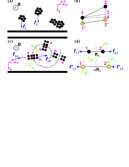
Figure 1: (Color online) (a) Migration of flocs towards the walls in a laminar flow. (b) Schematics of the distance change between two flocs after magnetic field is applied. Position- $1$ and $2$ are the positions of the two flocs without a magnetic field. Position- $1^{\prime}$ and $2^{\prime}$ are the positions of the two flocs with a magnetic field after time $t$. Obviously, distance-$1^{\prime}2^{\prime}$ is somewhat shorter than distance-$12$. (c) Self-rotation of a floc in a turbulent flow. The dashed line is a vorticity orbit while the solid line separates the primary-particles into two groups, $a$ and $b$, which have opposite net vector velocity $u_{a}$ and $u_{b}$ with respect to the applied magnetic field, producing Lorentz forces with opposite directions $f_{La}$ and $f_{Lb}$. (d) Schematics of the distance change between two primary-particles in a floc after a magnetic field is applied. Before disruption, the distance is $R_{0}$ without a magnetic field but $\alpha R_{0}$ with a magnetic field. It is clear that $\alpha\geq 1$.

always drag the flocs toward the walls. This process is similar to the sedimentation effect that can be called as floc-migration (FM).

On the other hand, floc rotation in laminar flows [11] and velocity fluctuation in turbulent flows [5, 12] are inevitable. In most cases, the former one is neglected while the latter should be taken into account. As mentioned in Ref. 5, random velocity fluctuations may induce pressure difference on opposite sides of a floc, which causes its deformation and eventual rupture [5], i.e., it increases the distance between the primary-particles inside the floc. Thus, as shown in Fig. 1(c), we can expect that in a turbulent flow a floc moves along the circular orbit and spins around its center, showing floc-self-rotations (FSR). This is somewhat similar to the Earth orbital motion around the Sun combined with the Earth’s spinning around its axis. Such FSR causes the constituting primary-particles in the floc to have different net vector velocities. In this case we divide the floc into two parts, $a$ and $b$, which have opposite velocity directions $u_{a}$ and $u_{b}$. When a magnetic field is applied, the two velocities produce opposite Lorentz forces and induce an extra pressure difference (we identify it as magnet-induced stress) on opposite sides of the floc, which enhances the total stress (i.e. the total interaction energy $V_{T}$ between two primary-particles) under turbulent conditions, and thus stretches the floc to a more prolate spheroid. Once the total stress surpasses the yield stress of the floc, it breaks up.

In principle, we cannot directly estimate the FM and FSR effects by a special potential term as $V_{EL}$, $V_{VDW}$, and $V_{M}$ shown in Refs. 6, 7 because the Lorentz forces acted on different charged particles are independent from each other. But, by means of the distance change between the flocs due to the FM effect, or between the primary-particles inside a floc due to the FSR effect we can estimate the total energy change in Eq. (1). To do this, we need to know the velocity distribution in each position at every time. The most precise way is to solve the Navier-Stokes equations by computational fluid dynamics (CFD) softwares. But this is a quite complicated task and it goes beyond the scope of this work.

Fortunately, we can have two simple alternative ways to estimate the velocity distributions and hence the distance changes due to the magnetic effects. First, for the distance change between flocs caused by the FM effect, considering that this FM effect is dominant in laminar flows (also possible in weak turbulent flows), one can approximate the velocity in the $x$-direction along a 2-dimension (2$D$) pipe as

$$v_{x}=v_{max}(1-4y^{2}/D^{2}),$$ (2)

where $v_{max}$ is the maximum linear velocity at the center part of the pipe, and $D$ is the diameter of the pipe. Then, from the physical viewpoint, the dynamics of an isolated floc in $y$-direction is governed by the Newtonian equation as

$$F_{Gravity,y}+F_{Lorentz,y}+F_{viscosity,y}=m_{f}\frac{d^{2}y}{dt^{2}},$$ (3)

where $F_{Gravity,y}$ is the gravity force, $F_{Lorentz,y}$ is the Lorentz force, $F_{viscosity,y}$ is the friction force of the fluid, and $m_{f}$ and $y$ are the mass and translation of the floc, respectively.

If $F_{Lorentz,y}<<F_{Gravity,y}$, the system is reduced to the sedimentation case and the velocity and moving distance in $y$-direction, $v_{y}$ and $y$, are mainly dependent on the gravity force. Thus, at steady state, one can easily find that [7], $v_{y}=\frac{dy}{dt}=\frac{2g}{9\mu}(\rho_{particle}-\rho_{fluid})a_{f}^{2}$, and $y=y_{0}+\frac{2g}{9\mu}(\rho_{particle}-\rho_{fluid})a_{f}^{2}t$, where $\rho_{particle}$ and $\rho_{fluid}$ are the densities of the floc and the fluid, respectively, $a_{f}$ is the radius of the floc, $g$ is the gravity constant, $\mu$ is the viscosity of the fluid, and $t$ is the integral time.

However, in modern nano-dispersion systems the relation $F_{Lorentz,y}>>F_{Gravity,y}$ is often satisfied since the gravity effect can be neglected. Similarly, by using Eqs. (2) and (3) the $v_{y}$ and $y$ can be estimated as,

$$v_{y}=\frac{dy}{dt}=\frac{AD[-1+tanh(At)^{2}](D^{2}-4y_{0}^{2})}{2[D-2y_{0}tanh(At)]^{2}},$$ (4a)

$$y=\frac{2y_{0}D-D^{2}tanh(At)}{2D-4y_{0}tanh(At)},$$ (4b)

where $A=qNB_{z}v_{max}/(3\pi a_{f}\mu D)$, $q$ is the elementary charge constant, and $N$ is the total charge number in the floc which is associated with the potential of the surface charges, $\psi_{0}$.

Consequently, combining Eq. (2) and (4) we can estimate the position of a floc flowing in a laminar flow at any time due to the FM effect. Fig. 1(b) is the schematic presentation of two flocs migrating in a 2$D$ pipe. Position- $1$ and $2$ are the originals of the two flocs. As it can be seen, without magnetic field the $y$ coordinates are not changed, while with magnetic field the flocs move to position- $1^{\prime}$ and $2^{\prime}$, respectively, after time $t$. Obviously, distance-$1^{\prime}2^{\prime}$ is somewhat shorter than distance-$12$. To trace in a better way the distance change by the magnetic field we introduce a ratio $\alpha=\frac{distance-1^{\prime}2^{\prime}}{distance-12}$. This $\alpha$ is clearly dependent on magnetic field, and potential of the surface charge. For such FM case $\alpha$ is smaller than 1.

Secondly, the distance change between the primary-particles inside a floc, due to the FSR effect which dominates in turbulent flows, can also be estimated in a simple way. Notice that before a floc breaks the extra stress (force), for instance, the magnetic-induced stress inside the floc is always relaxed by the distance change. For simplicity we only discuss pair interaction between any two primary-particles as the classic DLVO theory did to estimate the distance change between the pairs. Fig. 1(d) is the schematic presentation of the distance change between two primary-particles inside a floc induced by magnetic field. We assume that these two primary-particles are balance at positions $1$ and $2$ without magnetic field and at positions $1^{\prime}$ and $2^{\prime}$ with magnetic field. The distances between them are $R_{0}$ and $\alpha R_{0}$, respectively. For a given turbulent dispersion system without magnetic field, if we assume that the length and time scales are the order of Kolmogorov length and time scales, respectively, the distribution of the intensity of turbulence over the range of wavenumbers (or over the range of eddy sizes) can be determined as follow [12],

$$\frac{3}{2}u^{2}_{1,2}=\int_{k}^{\infty}E(k,t)dk,$$ (5)

where $u_{1,2}$ is the fluctuation velocity, $k$ is the wavenumber (reciprocal of the characteristic length $r$), and $E(k,t)=const.\times\epsilon^{2/3}k^{-5/3}$ for $\eta\ll r\ll L$ while $\eta$ is the Kolmogorov length scale and $L$ is the large scales. Therefore, before disruption the distance between any two primary-particles, $R_{0}$, inside a floc is governed by the force balance equation acting at one primary-particle as,

$$\left.\frac{\frac{1}{2}m_{1,2}u_{1,2}^{2}}{R_{0}/2}=-\frac{dV_{T}}{ds}\right|_{s=R_{0}/a},$$ (6)

where $m_{1,2}$ is the mass of primary-particles. The left-hand side is the force caused by the kinetic energy of the turbulence while the right-hand side is the static force caused by the total interaction potential. Similarly, for a system with a magnetic field, the force balance is changed to,

$$\left.\frac{\frac{1}{2}m_{1,2}u_{1,2}^{\prime 2}}{\alpha R_{0}/2}+qN_{0}u^{\prime}_{1,2}B_{z}=-\frac{dV_{T}}{ds}\right|_{s=\alpha R_{0}/a},$$ (7)

where $u^{\prime}_{1,2}$ is the fluctuation velocity with a magnetic field, and $N_{0}$ is the total charge number in the primary- particle. The second term in the left-hand side is the Lorentz force. Furthermore, before disruption, the change of the total interaction potential must equal to the change of the kinetic energy (energy conservation),

$$V_{T}(\alpha R_{0})-V_{T}(R_{0})=\frac{1}{2}m_{1}(u_{1}^{\prime 2}-u_{1}^{2})+\frac{1}{2}m_{2}(u_{2}^{\prime 2}-u_{2}^{2}).$$ (8)

For simplicity, we further suppose that the primary-particles are identical, that is, $m_{1}=m_{2}=m_{pp}$, $|u_{1}|=|u_{2}|=|u|$ and $|u^{\prime}_{1}|=|u^{\prime}_{2}|=|u^{\prime}|$. Thus, combining Eqs. (1), (6), (7), and (8) we can calculate the four unknown variables, $V_{T}$, $R_{0}$, $u^{\prime}$, and $\alpha$. Obviously, this $\alpha$ is dependent also on the magnetic field, Reynolds number, and potential of the surface charge. In this case $\alpha$ is greater than 1, which means the floc is getting more prolate and less oscillating before it is broken apart.

Now we turn to the discussion of the effect of an external transverse magnetic field on the pair interaction potential curve. Fig. 2 presents the total energy with respect to the distance between two primary-particles. The solid line without symbol is the classic DLVO curve without magnetic field.

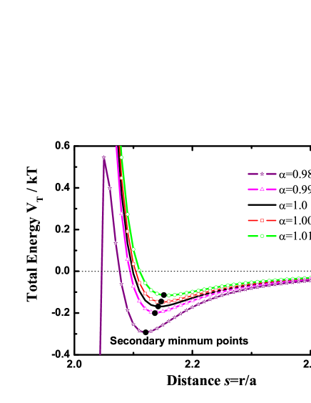
Figure 2: (Color online) Total energy with respect to the distance between two primary-particles. The solid black line without symbols is the classic DLVO curve without magnetic field. Solid curves with open star, triangle, square, and circle are the cases of $\alpha=0.985,0.995,1.005,and~{}1.015$, respectively. Black filled dots in each curve are the secondary minimum points.

Solid curves with open star, triangle, square, and circle are slight distance change cases, such as, $\alpha=0.985,0.995,1.005,and~{}1.015$, respectively. From the figure we can find that in laminar flow ($\alpha<1$), due to the FM effect, the curve produces a more pronounced secondary minimum which means that the interaction energy is more attractive than the one without magnetic field. In this case the flocs flocculate more easily from a relatively large interparticle distance, giving rise to a relatively large floc size, which is in a good agreement with the experimental results reported in Refs. 8, 9, 10. While in a turbulent flow ($\alpha>1$), due to the FSR effect, the curve is completely above the classic one which means that the total energy is less attractive than the one without magnetic field. In this case the original aggregates are elongated into prolate spheroids by the extra magnetic-induced stress and eventually break up into smaller flocs leading to a relatively small average floc size. This is the reason why the size of flocs is reduced in strong turbulent flows reported in Refs. 9, 10. Furthermore, in weak turbulent flows, both the FM and FSR effects are comparable. Thus, the floc size is dependent on the competition between FM and FSR. Using this model we can explain why the floc size increases in weak turbulent region in Refs. 9, 10: the FM effect in this case is stronger than the FSR.

3 Conclusions

To conclude, a transverse magnetic field results in Lorentz forces acting on primary-particles and hence flocs, which drag flocs toward the walls and/or elongate flocs into prolate spheroids. The former mechanism mainly works in laminar flows leading to a decrease of the distances between the flocs, while the latter dominates in turbulent flows thus giving rise to an increase of the distances between the primary-particles inside a floc. This model predicts that under MHD conditions, the size increases in laminar or gentle turbulent flows and decreases in turbulent regime. We believe that the presented model is not only applicable for physics and chemical engineering science, but also for the biology, medicine, etc. A good example here is the investigation of the stability of protein molecules. It should be noted here that the model in this paper is only one eddy for the regime of turbulence. Further stage calculations one should take into account many eddies of different sizes and a statistical description should be used.

4 Acknowledgement

This work was sponsored by K.U. Leuven Interdisciplinary research programme (IDO-project), IDO/04/009.

References

- [1] B. V. Derjaguin and L. Landau, Acta PhysicoChemica USSR, 14, 633 (1941).
- [2] E. J. W. Verwey and J. Th. G. Overbeek, Theory of the stability of Lyophobic Colloids, Elsevier, New York, 1948.
- [3] J. M. Montgomery, Consulting Engineers, “Water Treatment — Principles and Design”, Willey, New York, 1985.
- [4] Yerachmiel Argaman, and Warren J. Kaufman, J. Div. Saint. Eng.,Proc. Amer. Soc. Civil Eng. 96 (SA2), 223 (1970).
- [5] D. G. Thomas, AIChE J. 10, 517 (1963).
- [6] Jan Svoboda, IEEE Trans. Magn. MAG-18, 796 (1982).
- [7] M. R. Parker, R. P. A. R. van Kleef, H. W. Myron, and P. Wyder, IEEE Trans. Magn. MAG-18, 1647 (1982).
- [8] K. W. Busch, S. Gopalakrishnan, M. A. Busch, E. Tombcz, J. Coll. Interf. Sci. 183, 528 (1996).
- [9] Bernard Stuyven, Qinghua Chen, Wim Van de Moortel, Heiko Lipkens, Bart Caerts, Alexander Aerts, Lars Giebeler, Bernard Van Eerdenbrugh, Patrick Augustijns, Guy Van den Mooter, Jan Van Humbeeck, Johan Vanacken, Victor V. Moshchalkov, Jan Vermant and Johan A. Martens, Chem. Commun.,1, 47 (2009).
- [10] Bernard Stuyven, Gina Vanbutsele, Jan Nuyens, Jan Vermant, and Johan A. Martens, Chem. Eng. Sci., 64(8), 1904-1906, 2009.
- [11] H. L. Goldsmith, and S. G. Mason, “Rheology:Theory and Applications”, Academic Press, New York, 1967; S. G. Mason, J. Colloid Sci. 58, 275 (1977).
- [12] J. O. Heinze, Turbulence, McGraw-Hill, New York (1959).