Morse Theory for Geodesics in Conical Manifolds

Abstract

The aim of this paper is to extend the Morse theory for geodesics to the conical manifolds. In a previous paper [15] we defined these manifolds as submanifolds of $\mathbb{R}^{n}$ with a finite number of conical singularities. To formulate a good Morse theory we use an appropriate definition of geodesic, introduced in the cited work. The main theorem of this paper (see theorem 3.6, section 3) proofs that, although the energy is nonsmooth, we can find a continuous retraction of its sublevels in absence of critical points. So, we can give a good definition of index for isolated critical values and for isolated critical points. We prove that Morse relations hold and, at last, we give a definition of multiplicity of geodesics which is geometrical meaningful. In section 5 we compare our theory with the weak slope approach existing in literature. Some examples are also provided.
MSC Numbers: 58E05; 49J52; 58E10
Keywords: Geodesics, Morse Theory, Nonsmooth Analysis, Nonsmooth Manifolds

1 Introduction

In a previous work [15] we introduced conical manifolds as submanifolds of $\mathbb{R}^{n}$, giving the following definition:

Definition 1.1.

A conical manifold $M$ is a complete $n$-dimensional $C^{0}$ sub manifold of $\mathbb{R}^{m}$ which is everywhere smooth, except for a finite set of points $V$. A point in $V$ is called vertex.

These kind of manifold have many common features with other singular manifolds present in literature, as the Cone-manifolds studied by Hodgson and Tysk [17], the piecewise linear manifolds (see, e.g [1, 21, 22]), or the Orbifolds ([6, 5, 23]); in [16] these links are briefly examined.

Furthermore, the geodesic problem on a singular manifold is studied by Degiovanni and Morbini, in [12]. In section 5 we will point out the common feature and the main differences between our approach and the Degiovanni and Morbini one.

In our previous work we gave the following definition of geodesic, which seems to be appropriate for these kind of problems ([15, Definition 2]).

Definition 1.2.

A path $\gamma\in H^{1,2}([0,1],M)$ is a geodesic iff

• the set $T=T_{\gamma}:=\{s\in(0,1):\gamma(s)\in V\}$ is a closed set without internal part;

• $D_{s}\gamma^{\prime}=0\,\,\forall s\in[0,1]\smallsetminus T$;

• $|\gamma^{\prime}|^{2}$ is constant as a function in $L^{1}$.

By this definition, we were able to prove a deformation lemma that allows us to apply the main theorems of the calculus of variation in the large. In particular we can estimate the number of geodesics using the Ljusternik-Schnirelmann theory ([15, Theorem 1]).

In this work we will associate to each geodesic $\gamma$ an index $i(\gamma)$ similar to the Morse index, that allows us to obtain some information on the qualitative properties of the geodesics. By this index we state also an analogous of the Morse relations that hold in the smooth case.

As usual, given $p,q\in M$, we set

$${\Omega}={\Omega}_{p,q}:=\left\{\gamma\in W^{1,2}([0,1],\mathbb{R}^{n})|\gamma(0)=p,\gamma(1)=q,\gamma([0,1])\subset M\right\},$$

the suitable path space, and a functional

$$E:{\Omega}\rightarrow\mathbb{R}$$ (1)

$$E(\gamma)=\int\limits_{0}^{1}\|\gamma^{\prime}\|^{2}dt.$$ (2)

Moreover we set

$${\Omega}^{c}={\Omega}^{c}_{p,q}:=\left\{\gamma\in{\Omega},E(\gamma)\leq c\right\}.$$

$${\Omega}^{b}_{a}=\{{\Omega}_{p,q}\}^{b}_{a}:=\left\{\gamma\in{\Omega},a\leq E(\gamma)\leq b\right\}.$$

Under suitable assumption, if $M$ is a generic smooth manifold, we know that the following Morse relations hold.

$$\sum_{K\cap{\Omega}_{a}^{b}}\lambda^{m(\gamma)}={P}_{\lambda}({\Omega}^{a},{\Omega}^{b})+(1+\lambda){Q}_{\lambda}.$$ (3)

$$\sum_{K}\lambda^{m(\gamma)}={P}_{\lambda}({\Omega})+(1+\lambda){Q}_{\lambda}.$$ (4)

where $K$ is the set of geodesics, ${P}_{\lambda}(X,Y)$ is the Poincaré polynomial (in the variable $\lambda$) of the couple $(X,Y)$, ${Q}_{\lambda}$ is a formal series with coefficient in $\mathbb{N}\cup\{+\infty\}$, and $m(\gamma)$ is the Morse index of the geodesic $\gamma$, i.e. the signature of the second variation of the energy. Furthermore, if we take a geodesic $\gamma$ s.t. $E(\gamma)=c$ and ${\Omega}^{c+{\varepsilon}}_{c-{\varepsilon}}\cap K=\gamma$ for some ${\varepsilon}>0$, then we have that

$$\lambda^{m(\gamma)}={P}_{\lambda}({\Omega}^{c+{\varepsilon}},{\Omega}^{c-{\varepsilon}})$$ (5)

(for some references on Morse theory the reader can check, for example [19], [2, 3, 4],[8]).

Coming back to conical manifold, the usual definition of $m(\gamma)$ makes no sense since the energy is not differentiable. However, under suitable assumptions, we can define the index of a geodesic as the formal polynomial

$$i(\gamma)={P}_{\lambda}({\Omega}^{c+{\varepsilon}},{\Omega}^{c-{\varepsilon}}),$$ (6)

according to (5). In this case the Morse relations (3) and (4) become

$$\sum_{K\cap{\Omega}_{a}^{b}}i(\gamma)={P}_{\lambda}({\Omega}^{a},{\Omega}^{b})+(1+\lambda){Q}_{\lambda}.$$ (7)

$$\sum_{K}i(\gamma)={P}_{\lambda}({\Omega})+(1+\lambda){Q}_{\lambda}.$$ (8)

In this work we prove that $i(\gamma)$ is a good definition, i.e. does not depends on ${\varepsilon}$ and that (7) and (8) hold.

We have also that, while in a smooth manifold, for a generic geodesic, $i(\gamma)$ is a monome in $\lambda$, for a geodesic in a conical manifold this is not true. Then we have introduce the multiplicity of a geodesic (Definition 4.5) as

$$\operatorname{mult}({\gamma})=i(\gamma)|_{\lambda=1}.$$ (9)

we show some examples in which an high multiplicity, or a 0 multiplicity of a geodesic occurs.

Also, the definition of index that we give, allows us to make a comparison between our approach to conical manifold and the approach of Degiovanni, Marzocchi and Morbini (Section 5), which is based on the concept of the weak slope (see [7, 9, 10, 11]), and was presented in [12, 18]

2 Preliminary Results

In this section we present some peculiarities of the study of geodesics in conical manifold, which motivate Definition 1.2. Also, we resume briefly some result contained in [15] which will be useful for this paper.

Usually there are two ways to introduce geodesics in a smooth manifolds: at first we can formulate a Cauchy problem, i.e., given $p\in M$, $v\in T_{p}M$, we look for a continuous curve $\gamma:I\rightarrow M$ s.t.

$$\left\{\begin{array}[]{l}D_{s}\gamma^{\prime}=0;\\ \gamma(0)=p;\\ \gamma^{\prime}(0)=v.\end{array}\right.$$ (10)

Otherwise we can choose a suitable path space and an energy functional, for example, the space ${\Omega}$ and the functional $E$ previously defined, and we look for critical points of the energy.

Contrarily to the smooth case, these two methods are not equivalent for manifolds which have conical singularities, and each one of them have some peculiarity. If we try to solve the Cauchy problem we have neither uniqueness nor continuous dependence from starting condition: David Stone (see [21], [22]) showed that there are piecewise linear manifold with a vertex $p$ (indeed a special case of conical manifolds) in which, given a point $q$, there is a family of minimal geodesics solving (10) that are the same straight line between $q$ and $p$, then start again from $p$ with different angles. So (10) has many solutions, and there is no reasonable criterion to choose one of these geodesics instead of another.

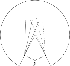
Figure 1: Geodesics starting from a point.

Now, taken an Euclidean half cone, we can represent it as a circular sector in a plane, in which the straight edges are identified. Taking $p$ on these edges, we represent the geodesics as straight lines starting from $p$. In Fig. 1 we show two sequence of geodesics, respectively the continuous and the dotted lines, approaching the edges of the circular sector. It is easy to see that a dotted and a continuous line can not be too close, even if they approach the geodesic which start from $p$ and goes to the vertex. Even in a familiar case we are not able to say how can a geodesic pass through the vertex, in order to have continuous dependence from initial data.

Also, if we take two points, say $p$ and $q$, symmetrical respect to the vertex, we can say that there are always two minimal geodesics joining them, even if $p$ and $q$ are as close as we want; so it is not possible to define a normal neighborhood of the vertex. Thus we can not hope to define a global exponential map.

The functional approach, on the contrary, gives us an easy result on minimal geodesics. To finding minima is useful to extend $E$ in the whole space

$$W^{1,2}_{p,q}:=\left\{\gamma\in W^{1,2}([0,1],\mathbb{R}^{n})|\ \gamma(0)=p,\gamma(1)=q\right\}$$ (11)

and to look at minima of $E$ with the constraint $\text{Im}(\gamma)\subset M$; in this way we know that $E$ is lower semi continuous for the $W^{1,2}$-weak topology and the set $\big{\{}\gamma|\gamma\in{\Omega}\cap W^{1,2}_{p,q},\,\|\gamma\|_{W^{1,2}}<c\big{\}}$ is weakly compact in $W^{1,2}_{p,q}$, because $M$ is complete: then the problem

$$\min_{\begin{subarray}{c}\gamma\in W^{1,2}_{p,q}\\ \text{Im}\gamma\subset M\end{subarray}}E(\gamma)$$ (12)

has a solution, and we can formulate the following theorem.

Theorem 2.1.

Let $M$ be a conical manifold; let $p,q\in M$.

Then, the energy functional

$$\begin{array}[]{c}E:{\Omega}_{p,q}\rightarrow\mathbb{R}\\ E(\gamma)=\int\limits_{0}^{1}\|\gamma^{\prime}\|^{2}dt.\end{array}$$ (13)

has a minimum.

Proof.

Just proved. ∎

However, this approach is not completely useful, because the energy is not smooth, so there is no easy way to define a critical point of energy different from minimum. In the cited work we gave a generalized definition of geodesic (Definition 2) which seems to be the right one for these kind of problems.

In fact, although this is a local definition, it let us show two deformation lemmas typical of the calculus of variation in the large ([15, Theorem 2 and Theorem 7]). This lemmas are crucial for this work and are briefly recalled here. In the next section we will provide also some sketch of the proof of these results.

Lemma 2.2 (First deformation lemma).

Let $M$ be a conical manifold, and let $p,q\in M$. Suppose that there exists $c>0$ s.t. there are a finite number of geodesics with energy lesser than $c$. Suppose also that there are no geodesics which energy is in the strip $[a,b]$ for some $a,b\in\mathbb{R}$, $a<b<c$. Then ${\Omega}^{a}$ is a deformation retract of ${\Omega}^{b}$.

Lemma 2.3 (Second deformation lemma).

Let $M$ be a conical manifold, $p,q\in M$. Suppose that there exists $c>0$ s.t. there are a finite number of geodesics with energy lesser than $c$. Suppose also that there are no geodesics which energy is in the strip $[a,b)$ for some $a,b\in\mathbb{R}$, $a<b<c$. Set $k_{b}$ the set of $b$-energy geodesics, then there exists a neighborhood $U$ of $k_{b}$ s.t.

$${\Omega}^{b}\smallsetminus U\simeq{\Omega}^{a}.$$

These results link the topological structure of sublevels of $E$ with our definition of geodesics and allow us to consider geodesics as critical points of energy. By these lemmas, in the cited work we proved an estimate on the number of geodesic in a conical manifold, via the Ljusternik-Schnirelmann theory. In this paper these lemmas allow us to prove that the definition of the index $i(\gamma)$ is a good definition.

3 Morse Theory For Critical Levels

In order to define the index of a critical point and of a critical level, we recall the definition of Poincaré polynomial

Definition 3.1.

Let $H^{*}$ the Alexander-Spanier cohomology with coefficient in a field ${\mathbb{F}}$. For every pair $(X,A)$ of closed spaces, the Poincaré polynomial is the formal series in the variable $\lambda$ (with the convention that $\lambda^{\infty}=0$)

$${P}_{\lambda}(X,A,{\mathbb{F}})={P}_{\lambda}(X,A)=\sum_{q=0}^{\infty}\dim H^{q}(X,A,{\mathbb{F}})\lambda^{q}.$$ (14)

Moreover, we set

$${P}_{\lambda}(X,{\mathbb{F}}):={P}_{\lambda}(X,\emptyset,{\mathbb{F}}).$$ (15)

For the main properties of the formal series we refer to [4]. We use the Alexander-Spanier cohomology (see [20] for an exhaustive treatment) to define the index of a geodesic because we need its continuity property (recalled in Theorem 4.2) to prove Theorem 4.3.

Definition 3.2.

Given $p,q\in M$, suppose that there exists a $\bar{c}$ s.t. ${\Omega}^{\bar{c}}$ contains a finite number of geodesics. Let $c<\bar{c}$. Set, as usual $k_{c}$ the set of $c$-energy geodesic, we define the index of $k_{c}$ as

$$i(k_{c})={P}_{\lambda}({\Omega}^{c+{\varepsilon}},{\Omega}^{c-{\varepsilon}}),$$ (16)

for ${\varepsilon}$ sufficiently small.

In order to prove that 3.2 is a good definition, we need to show now that there exists $\bar{\varepsilon}$ s.t. $\forall{\varepsilon}_{1}<{\varepsilon}_{2}\leq\bar{\varepsilon}$

$${P}_{\lambda}({\Omega}^{c+{\varepsilon}_{1}},{\Omega}^{c-{\varepsilon}_{1}})={P}_{\lambda}({\Omega}^{c+{\varepsilon}_{2}},{\Omega}^{c-{\varepsilon}_{2}}).$$

In order to prove it, we show that ${\Omega}^{c+{\varepsilon}_{2}}$ retracts on ${\Omega}^{c+{\varepsilon}_{1}}$ and that ${\Omega}^{c-{\varepsilon}_{1}}$ retracts on ${\Omega}^{c-{\varepsilon}_{2}}$. This is possible by the deformation lemmas (2.2 and 2.3) cited previously. Here we recall shortly the main tools of the proof.

We choose ${\varepsilon}$ s.t. $[c-{\varepsilon},c+{\varepsilon}]$ contains only $c$ as critical value. We start defining some special subset of ${\Omega}^{c+{\varepsilon}_{1}}_{c+{\varepsilon}_{2}}$ (for ${\Omega}^{c-{\varepsilon}_{2}}_{c-{\varepsilon}_{1}}$ we will act in the same way). Let

$$\Sigma=\{\gamma\in{\Omega}^{c+{\varepsilon}_{1}}_{c+{\varepsilon}_{2}},\text{ s.t. Im}\gamma\cap V\neq\emptyset\}$$ (17)

(we recall that $V$ is the set of vertexes). If $\gamma_{i}$ is a geodesic in ${\Omega}^{c+{\varepsilon}}$, let

$$\Sigma_{i}=\{\gamma\in\Sigma\text{ s.t. }\gamma=\gamma_{i}\text{ up to affine reparametrization }\}.$$ (18)

Lemma 3.3.

$\Sigma_{i}$ is compact for all $i$

Proof.

The proof is not difficult and can be found in ([15, Lemma 3]) ∎

By the compactness we can prove the following lemma.

Lemma 3.4 (existence of retraction in $\bigcup_{i}\Sigma_{i}$).

There exist $R\supset\bigcup_{i}\Sigma_{i}$, $\nu,\bar{t}\in\mathbb{R}^{+}$ and

$$\eta_{R}:R\times[0,\bar{t}\,]\rightarrow H^{1}(I,M)$$

a continuous function s.t.

• $\eta_{R}(\beta,0)=\beta$

• $E(\eta_{R}(\beta,t))-E(\beta)<-\nu t$

for all $t\in[0,\bar{t}\,]$, $\beta\in R$.

Proof.

The proof is quite technical, and is based on a modification of Degiovanni and Marzocchi techniques. For the details we refer to ([15, Lemma 4]) ∎

We can prove also a deformation result that is in some sense the complementary of the previous lemma.

Lemma 3.5.

For any $U\supset\bigcup_{i}\Sigma_{i}$ there exist $\bar{t},\nu\in\mathbb{R}^{+}$ and a continuous functional

$$\eta_{U}:{\Omega}^{c+{\varepsilon}_{1}}_{c+{\varepsilon}_{2}}\smallsetminus U\times[0,\bar{t}\,]\rightarrow{\Omega}^{c+{\varepsilon}_{1}}_{c+{\varepsilon}_{2}}$$

such that

• $\eta_{U}(\cdot,0)=\text{Id}$

• $E(\eta_{U}(\beta,t))-E(\beta)\leq-\nu t$

for all $t\in[0,\bar{t}\,]$, for all $\beta\in{\Omega}^{c+{\varepsilon}_{1}}_{c+{\varepsilon}_{2}}\smallsetminus U$

Proof.

We use that for every $\gamma\in\Sigma\smallsetminus U$ we can find a vector field $w_{\gamma}$ s.t. $dE(\gamma)[w_{\gamma}]$ exists, although the energy is not smooth. Moreover, outside $\Sigma$ the energy can be differentiated, so we can use pseudo gradient vector field construction and we find the wanted retraction (for all details see [15, Lemma 5]) ∎

From Lemma 3.4 and Lemma 3.5 we get the following result, which states that Definition 3.2 is a good definition.

Theorem 3.6.

Let $M$ be a conical manifold, let $p,q\in M$ be s.t. $E$ admits only a finite set of critical points under a certain level $\bar{c}$. Let $c<\bar{c}$ be a critical level. There exists an ${\varepsilon}>0$ s.t., for any ${\varepsilon}_{1},{\varepsilon}_{2}<{\varepsilon}$, we have that

$${P}_{\lambda}({\Omega}^{c+{\varepsilon}_{1}},{\Omega}^{c-{\varepsilon}_{1}})={P}_{\lambda}({\Omega}^{c+{\varepsilon}_{2}},{\Omega}^{c-{\varepsilon}_{2}}).$$ (19)

Proof.

Because there are a finite number of critical points, we can choose ${\varepsilon}$ s.t. $[c-{\varepsilon},c+{\varepsilon}]$ contains only $c$ as critical value. Chosen ${\varepsilon}_{1}<{\varepsilon}_{2}<{\varepsilon}$, we want to retract ${\Omega}^{c+{\varepsilon}_{2}}$ on ${\Omega}^{c+{\varepsilon}_{1}}$ and ${\Omega}^{c-{\varepsilon}_{1}}$ on ${\Omega}^{c-{\varepsilon}_{2}}$. Defined as before $\Sigma$ and $\Sigma_{i}$ in ${\Omega}^{c+{\varepsilon}_{2}}_{c+{\varepsilon}_{1}}$, we note that for $i\neq j$ then $\Sigma_{i}\cap\Sigma_{j}=\emptyset$, because the geodesics $\gamma_{i}$ and $\gamma_{j}$ are distinct. Set $N$ the number of critical points under the level $c+{\varepsilon}$, we can find a neighborhood $R\supset\bigcup\limits_{i}\Sigma_{i}$ and a retraction $\eta_{R}$ as in Lemma 3.4. Furthermore, for every $U\supset\bigcup\limits_{i=0}^{N}\Sigma_{i}$ there exists a retraction $\eta_{U}$ on ${\Omega}^{c+{\varepsilon}_{2}}_{c+{\varepsilon}_{1}}\smallsetminus U$ in analogy with Lemma 3.5. We choose $U$ s.t. there exists $V$ a neighborhood of $\bigcup\limits_{i}\Sigma_{i}$ with

$$\bigcup_{i}\Sigma_{i}\subsetneq U\subsetneq V\subsetneq R.$$

For the sake of simplicity we will suppose that $\eta_{U}$ and $\eta_{R}$ are defined for $0\leq t\leq 1$ and that $\nu$ is the same for both of them. Let $\theta_{1}:{\Omega}^{c+{\varepsilon}_{2}}\rightarrow[0,1]$ be a continuous map s.t.

$$\theta_{1}|_{U}\equiv 0;$$

$$\theta_{1}|_{{\Omega}^{c+{\varepsilon}_{1}}\smallsetminus V}\equiv 1.$$

Then we define a continuous map

$$\mu_{1}:{\Omega}^{c+{\varepsilon}_{2}}\times[0,1]\rightarrow{\Omega}^{c+{\varepsilon}_{2}},$$ (20)

$$\mu_{1}(\beta,t)=\eta_{U}(\beta,\theta_{1}(\beta)t);$$ (21)

we know that $E(\mu_{1}(\beta,t))-E(\beta)\leq-\nu t\theta_{1}(\beta)$, so

$$\mu_{1}({\Omega}^{c+{\varepsilon}_{2}},1)\subset V\cup{\Omega}^{c+{\varepsilon}_{2}-\nu},$$

in fact if $\mu_{1}(\beta,t)\notin V$ for all $t$, then $E(\mu_{1}(\beta,t))-E(\beta)\leq-\nu t$, so $\mu_{1}(\beta,1)\in{\Omega}^{c+{\varepsilon}_{2}-\nu}$.

By $\mu_{1}$ we have retracted ${\Omega}^{c+{\varepsilon}_{2}}$ on ${\Omega}^{c+{\varepsilon}_{2}-\nu}\cup V$; now we define a continuous map $\theta_{2}:{\Omega}^{c+{\varepsilon}_{2}}\rightarrow[0,1]$ s.t.

$$\theta_{1}|_{{\Omega}^{c+{\varepsilon}_{2}}_{c+{\varepsilon}_{2}-\nu/2}}\equiv 1;$$

$$\theta_{1}|_{{\Omega}^{c+{\varepsilon}_{1}-\nu}}\equiv 0.$$

Then set

$$\mu_{2}:V\cup{\Omega}^{c+{\varepsilon}_{2}-\nu}\times[0,1]\rightarrow{\Omega}^{c+{\varepsilon}_{2}},$$ (22)

$$\mu_{2}(\beta,t)=\eta_{R}(\beta,\theta_{2}(\beta)t);$$ (23)

$\mu_{2}$ is a continuous map that retracts $V\cup{\Omega}^{c+{\varepsilon}_{2}-\nu}$ on ${\Omega}^{c+{\varepsilon}_{2}-\nu/2}$. By iterating this algorithm we can retract continuously ${\Omega}^{c+{\varepsilon}_{2}}$ on ${\Omega}^{c+{\varepsilon}_{1}}$.

The retraction of ${\Omega}^{c-{\varepsilon}_{1}}$ on ${\Omega}^{c-{\varepsilon}_{2}}$ is obtained in the same way. ∎

Remark 3.7.

The hypothesis of finiteness of critical points seems quite restrictive. Indeed, because we have a finite number of vertexes, in many concrete examples this assumption is easily verified, as shown in the applications.

To conclude this section we show some properties of ${P}_{\lambda}$ useful in the next.

Lemma 3.8.

(see [2, lemma 4.2,(v)]). Let $X$ a metric space, $A,B$ two closed subspace of $X$ s.t. $B\subset A\subset X$; then there exist a formal series ${Q}_{\lambda}$ s.t.

$${P}_{\lambda}(X,A)+{P}_{\lambda}(A,B)={P}_{\lambda}(X,B)+(1+\lambda){Q}_{\lambda}.$$ (24)

Proof.

We consider the exact sequence relative to the triple $X,A,B$:

$$\ldots\stackrel{{\scriptstyle\delta^{*}_{q-1}}}{{\longrightarrow}}H^{q}(X,A)\stackrel{{\scriptstyle i^{*}_{q}}}{{\longrightarrow}}H^{q}(X,B)\stackrel{{\scriptstyle j^{*}_{q}}}{{\longrightarrow}}H^{q}(A,B)\stackrel{{\scriptstyle\delta^{*}_{q}}}{{\longrightarrow}}\ldots$$ (25)

and we set

$$\begin{array}[]{c}a_{q}=\dim(\ker i^{*}_{q}),\\ b_{q}=\dim(\ker j^{*}_{q}),\\ c_{q}=\dim(\ker\delta^{*}_{q}).\end{array}$$

By exactness of (25) we have that

$$\begin{array}[]{rcl}\dim H^{q}(X,A)&=&a_{q}+c_{q-1};\\ \dim H^{q}(X,B)&=&a_{q}+b_{q};\\ \dim H^{q}(A,B)&=&b_{q}+c_{q},\end{array}$$

thus

$$\begin{array}[]{rcl}{P}_{\lambda}(X,A)&=&\sum_{q=0}^{\infty}(a_{q}+c_{q-1})\lambda^{q};\\ {P}_{\lambda}(X,B)&=&\sum_{q=0}^{\infty}(a_{q}+b_{q})\lambda^{q};\\ {P}_{\lambda}(A,B)&=&\sum_{q=0}^{\infty}(b_{q}+c_{q})\lambda^{q}.\end{array}$$

So

$${P}_{\lambda}(X,A)+{P}_{\lambda}(A,B)={P}_{\lambda}(X,B)+\sum_{q=0}^{\infty}(c_{q}+c_{q-1})\lambda^{q},$$ (26)

but we can write

$$\sum_{q=0}^{\infty}(c_{q}+c_{q-1})\lambda^{q}=(1+\lambda)\sum_{q=0}^{\infty}c_{q}\lambda^{q},$$ (27)

and then, by setting ${Q}_{\lambda}=\sum_{q=0}^{\infty}c_{q}\lambda^{q}$, we conclude the proof. ∎

Lemma 3.9.

(see [3, theorem II.3.5]) Let $M$ a conical manifold. If $M$ is topologically trivial, then also ${\Omega}$ is topologically trivial, thus

$${P}_{\lambda}({\Omega})=1.$$

Proof.

Obvious. ∎

By lemma 3.8 we can formulate the Morse relations for critical levels.

Theorem 3.10.

Let $M$ a conical manifold; let $p,q\in M$ s.t. $E$ admits only a finite number of critical points for every sublevel ${\Omega}^{c}$

Then, if $a$ and $b$ are regular levels there exists a formal series ${Q}_{\lambda}$ such that

$$\sum_{c\text{ critical in }(a,b)}i(k_{c})={P}_{\lambda}({\Omega}^{a},{\Omega}^{b})+(1+\lambda){Q}_{\lambda}.$$ (28)

Moreover, if we consider the whole space ${\Omega}$ there exists a ${Q}_{\lambda}$ such that

$$\sum_{c\text{ critical}}i(k_{c})={P}_{\lambda}({\Omega})+(1+\lambda){Q}_{\lambda}.$$ (29)

Proof.

We know that there is a finite set, say $\{c_{1},\cdots,c_{l}\}$, of critical levels in $[a,b]$. We can, by previous theorem, iterate (24) obtaining that

$$\sum_{j=1}^{l}i(k_{c_{j}})={P}_{\lambda}({\Omega}^{c_{l+{\varepsilon}}},{\Omega}^{c_{1-{\varepsilon}}})+(1+\lambda){Q}_{\lambda}.$$ (30)

Then by deformation lemma we obtain (28).

Finally, by a limiting process, and considering that ${\Omega}^{-1}=\emptyset$ we can prove (29) (we recall that, by definition, ${P}_{\lambda}({\Omega},\emptyset)={P}_{\lambda}({\Omega})$). ∎

4 Morse Theory For Geodesics

In this section we will define the Morse index for an isolated geodesics and finally prove, as claimed, the Morse relations. Under some a priori bound on the number of geodesics, we obtain an analogous of the Morse relations that holds in the smooth case.

Definition 4.1.

Let $c$ an isolated critical value. Let $k_{c}$ the set of $c$ energy geodesics and let $\gamma$ an isolated point of $k_{c}$. Then

$$i(\gamma)={P}_{\lambda}({\Omega}^{c},{\Omega}^{c}\smallsetminus\gamma)$$ (31)

To proceed, we need to recall the continuity property of Alexander-Spanier cohomology (see [20, Cor. 6.6.3]).

Theorem 4.2.

Let $X\supset A\supset B$, $X$ a paracompact Hausdorff space, $A,B$ closed in $X$.Then

$$\operatorname*{lim_{\rightarrow}}_{(U,V)\supset(A,B)}H^{q}(U,V)=H^{q}(A,B).$$ (32)

We can prove now the main theorem of this paper.

Theorem 4.3.

Let M a conical manifold. let $p,q\in M$ s.t. $E$ admits only a finite set of geodesics for every sublevel ${\Omega}^{c}$.

Then, if $a,b$ are regular values, we have

$$\sum_{\gamma\in{\Omega}_{a}^{b}\text{ geodesic}}i(\gamma)={P}_{\lambda}({\Omega}^{a},{\Omega}^{b})+(1+\lambda){Q}_{\lambda}.$$ (33)

Furthermore, if we consider the whole space we obtain

$$\sum_{\gamma\text{ geodesic}}i(\gamma)={P}_{\lambda}({\Omega})+(1+\lambda){Q}_{\lambda}.$$ (34)

Proof.

We know, by theorem 3.10 that

$$\sum_{c\text{ critical in }(a,b)}i(k_{c})={P}_{\lambda}({\Omega}^{a},{\Omega}^{b})+(1+\lambda){Q}_{\lambda};$$

where

$$i(k_{c})={P}_{\lambda}({\Omega}^{c+{\varepsilon}},{\Omega}^{c-{\varepsilon}}).$$

Because the critical point are in a finite number, we can choose $d$ s.t., if $i\neq j$, $B(\gamma_{i},d)\cap B(\gamma_{j},d)=\emptyset$. Setting $B_{k_{c}}(d)=\bigcup_{\gamma\in k_{c}}B_{\gamma}$, we have obviously, by the second deformation lemma, that ${\Omega}^{c-{\varepsilon}}\simeq{\Omega}^{c}\smallsetminus B_{k_{c}}(d)$, thus

$${P}_{\lambda}({\Omega}^{c+{\varepsilon}},{\Omega}^{c-{\varepsilon}})={P}_{\lambda}({\Omega}^{c+{\varepsilon}},{\Omega}^{c}\smallsetminus B_{k_{c}}(d)).$$

Then, by the continuity property of the Alexander-Spanier cohomology (Theorem 4.2) we have

$${P}_{\lambda}({\Omega}^{c+{\varepsilon}},{\Omega}^{c}\smallsetminus B_{k_{c}}(d))={P}_{\lambda}({\Omega}^{c},{\Omega}^{c}\smallsetminus B_{k_{c}}(d)).$$

To obtain the proof we want to show that

$$H^{*}({\Omega}^{c},{\Omega}^{c}\smallsetminus B_{k_{c}}(d))\simeq H^{*}({\Omega}^{c},{\Omega}^{c}\smallsetminus k_{c}).$$

It’s easy to see that both ${\Omega}^{c}\smallsetminus B_{k_{c}}(d)$, ${\Omega}^{c}\smallsetminus k_{c}$ are locally contractible subsets, so there is an isomorphism between Alexander-Spanier and singular cohomology $\bar{H}^{*}$ (see [20, Chap.6,Sec.9]). Furthermore, according to Definition 3.1, we are working with coefficient in a field ${\mathbb{F}}$, so there is also an isomorphism between $\bar{H}^{*}$ and $\operatorname{Hom}(\bar{H}_{*})$ (see [20, Th.5.5.3]). So it is enough to show that

$$\operatorname{Hom}(H_{*}({\Omega}^{c},{\Omega}^{c}\smallsetminus B_{k_{c}}(d)))\simeq\operatorname{Hom}(H_{*}({\Omega}^{c},{\Omega}^{c}\smallsetminus k_{c})).$$

Given $\omega\in H_{*}({\Omega}^{c},{\Omega}^{c}\smallsetminus k_{c})$, we know that $\omega\in H_{*}({\Omega}^{c},{\Omega}^{c}\smallsetminus B_{k_{c}}(d))$ for a sufficiently small $d$, because $\omega$ has compact support. So

$$H_{*}({\Omega}^{c},{\Omega}^{c}\smallsetminus k_{c})=\operatorname*{lim_{\rightarrow}}_{d}H_{*}({\Omega}^{c},{\Omega}^{c}\smallsetminus B_{k_{c}}(d)),$$

but $H_{*}({\Omega}^{c},{\Omega}^{c}\smallsetminus B_{k_{c}}(d))$ is definitely constant in $d$, thus we have that

$$H_{*}({\Omega}^{c},{\Omega}^{c}\smallsetminus B_{k_{c}}(d))=H_{*}({\Omega}^{c},{\Omega}^{c}\smallsetminus k_{c}).$$

We proved that

$${P}_{\lambda}({\Omega}^{c+{\varepsilon}},{\Omega}^{c-{\varepsilon}})={P}_{\lambda}({\Omega}^{c},{\Omega}^{c}\smallsetminus k_{c}).$$

Finally, by excision, we obtain

$${P}_{\lambda}({\Omega}^{c},{\Omega}^{c}\smallsetminus k_{c})=\bigoplus_{\gamma\in k_{c}}{P}_{\lambda}({\Omega}^{c},{\Omega}^{c}\smallsetminus\gamma)=\sum_{\gamma\in k_{c}}i(\gamma)$$

that proves (33). As usual by a limiting process we prove (34). ∎

Remark 4.4.

Following the proof of the above theorem, it’s easy to see that, if $k_{c}=\{\gamma\}$, then $i(k_{c})=i(\gamma)$, so the definition of index for a geodesic and for a critical set are compatible.

By the index we can also define the multiplicity of a critical point.

Definition 4.5.

Let $\gamma$ an isolated critical point of energy. Then

$$\operatorname{mult}(\gamma)=i(\gamma)|_{\lambda=1}.$$

It is well known that the geodesics with high multiplicity are unstable in smooth manifolds, i.e. up to small perturbations of extremal points $p$ and $q$ we can find only isolated geodesics, that have multiplicity 1. For conical manifolds this is false.

We will show in the next example, that in some cases, given $p,q$ on a conical manifold $M$, there exists a geodesic $\gamma_{0}$ with $\operatorname{mult}(\gamma_{0})>1$ joining them; for a sufficiently small change of the boundary data $p,q$ we will obtain another geodesic with the same multiplicity of $\gamma_{0}$.

Example.

Let $C$ be a 2-dimensional Euclidean half cone embedded in $R^{3}$; let $p,q$ be two points of $C$ and let $v$ be its vertex. We want to estimate the number of standard geodesics between $p$ and $q$.

Figure 2: Geodesic on a Cone.

We represent $C$ as a circular sector in the plane: let $\alpha$ be the wideness of the sector; we see that, if $\alpha$ is sufficiently small, there are many regular geodesic joining $p$ and $q$ (see, for instance [13, exercise 6, section 4-7]), and the number of these geodesics depends on $p,q$ and $\alpha$. If $\alpha$ is bigger than $\pi$, on the contrary, we have an unique geodesic joining $p$ and $q$. We can also observe that all these curves have different energies, and that they are shorter than the broken straight line $\gamma_{0}$, which joins $p$ to $v$ and $v$ to $q$, as shown in Fig 2. Because the cone is flat, any one of these geodesics has Morse index 0. In this case classical Morse theory fails, in fact ${P}_{\lambda}=1$, because the cone is contractible (see lemma 3.9), so

$$\sum_{i=1}^{n}\lambda^{m(\gamma_{i})}=n=1+(1+\lambda){Q}_{\lambda}$$ (35)

and so there will be at least $n-1$ geodesics whose Morse index is 1: this is a contradiction. If use our definition of generalized geodesic (Definition 1.2) to estimate the number of critical points of energy, we see that we must consider all the classical geodesics $\gamma_{1}$,…,$\gamma_{n}$, plus the broken geodesic $\gamma_{0}$ (up to reparametrization). The critical levels are all distinct, so every geodesic is isolated and we can apply (34), which states that Morse relations hold. These estimates give us that

$$n+i(\gamma_{0})=1+(1+\lambda){Q}_{\lambda},$$ (36)

then

$${Q}_{\lambda}=n-1+{R}_{\lambda},$$ (37)

where ${R}_{\lambda}$ is a formal series with non negative coefficients.

So

$$i(\gamma_{0})\geq(n-1)\lambda,$$ (38)

and

$$\operatorname{mult}(\gamma_{0})\geq(n-1).$$ (39)

As claimed, we have a geodesic $\gamma_{0}$ with an high multiplicity. If we look at the definition of this curve, we have obviously that $\operatorname{mult}(\gamma_{0})$ is stable for small perturbations of $p$ and $q$.

The above example gives us also a geometrical interpretation of multiplicity, in fact, if we smooth $C$, classical Morse theory holds, and we will see exactly $\operatorname{mult}(\gamma_{0})$ geodesics appearing. We can think that, is some sense, this geodesics accumulates in $\gamma_{0}$.

Furthermore $\operatorname{mult}(\gamma_{0})$ depends on the wideness $\alpha$ and it is zero if $\alpha>\pi$. We have a change of topology of the energy sublevels only when $\operatorname{mult}(\gamma_{0})\neq 0$; this fact allows us another consideration that we clarify with the following example.

Example.

Let $M=\mathbb{R}^{2}$ be endowed with the usual scalar product and let $v=(0,0)$, $p=(0,1)$, $q=(1,0)$; obviously, the unique Riemannian geodesic between $p$ and $q$ is the straight line $pq$.

We can also consider $M$ as a conical manifold with vertex $v$, according to definition 1.1. We see that also the broken line $pvq$ is a geodesic following definition 1.2: this fact seems artificial. By Morse relations we prove that $i(pvq)=0$, in fact, $i(pq)=1$, and ${P}_{\lambda}=1$, thus

$$i(pvq)+1=1+(1+\lambda){Q}_{\lambda}.$$ (40)

Then even $\operatorname{mult}(pvq)=0$. The geodesic $pvq$, thus, does not affect the structure of the sublevels of energy: the multiplicity of a curve allows us to distinguish the geodesics as $pvq$ from the ones that are meaningful critical points of energy.

This example shows that, by the multiplicity, we also recover the geometrical meaning of geodesic that we lost in the starting definitions.

5 Comparison with weak-slope approach

To complete the our study about geodesics, we want to compare our approach with Degiovanni-Marzocchi-Morbini one. These authors in [12, 18] study the problem of finding geodesics in manifolds with boundary by using the weak slope theory; under certain hypothesis on the conical manifold, both approaches are possible. We’ll see that there is a strong bound between these theories, and we’ll be able to recover a regularity result. Let $M$ be a conical manifold embedded in $\mathbb{R}^{n}$, and assume that $M$ is the Lipschitz boundary of an open convex set $A\subset\mathbb{R}^{n}$. Let $C=\mathbb{R}^{n}\smallsetminus A$, and let $p,q\in M\subset C$. We set the functional space

$$X=\{\gamma\in H^{1}([0,1],C),\gamma(0)=p,\gamma(1)=q\},$$

and we define a functional

$$\begin{array}[]{c}J:L^{2}([0,1],\mathbb{R}^{n})\rightarrow\mathbb{R}\cup\{\infty\},\\ \\ J(\gamma)=\left\{\begin{array}[]{ll}\int_{0}^{1}|\gamma^{\prime}|^{2}&\text{ if }\gamma\in X\\ +\infty&\text{ otherwise},\end{array}\right.\end{array}$$ (41)

in order to have the P.S. condition for every sublevel $J^{c}$.

Definition 5.1.

A curve $\gamma$ is a critical point of $J$ iff $|dJ|(\gamma)=0$, where $|dJ|$ is the weak slope introduced in [11].

We have that

Theorem 5.2.

Let $\gamma\in X$ be a critical point for $J$. Then

• $|\gamma^{\prime}|$ is constant almost everywhere.

• $\forall(a,b)\subset[0,1]$ we have that $\gamma^{\prime}\in BV((a,b),\mathbb{R}^{n})$ and there exists a finite Borel measure $\mu$ on $(a,b)$ and a bounded Borel function $\nu:(a,b)\rightarrow\mathbb{R}^{n}$ s.t $\nu(s)\in N_{\gamma(s)}C$ (the Clarke normal cone to $C$) for $\mu$ a.e. $s\in(a,b)$ such that

  $$\int_{a}^{b}|\gamma^{\prime}|ds=-\int_{a}^{b}\nu\delta d\mu$$

  $\forall\delta\in W^{1,1}((a,b),\mathbb{R}^{n})$ (i.e. in a distributional sense $\gamma^{\prime\prime}=\nu d\mu$)

Proof.

This theorem is a reformulation of [12, th.3.5] and[18, th.2.10], which we refer to. ∎

We can prove now the following proposition, that states a link between our approach and weak slope one.

Proposition 5.3.

Let $M$ be a conical manifold as above, and let $p,q\in M$. Let $E$ be defined as usual in (2). Suppose that exist a $\gamma\in{\Omega}$ and an ${\varepsilon}>0$ s.t. $\gamma$ is the unique geodesic (in the sense of Definition 1.2) in the strip ${\Omega}^{c+{\varepsilon}}_{c-{\varepsilon}}$, where $c=E(\gamma)$.

If $i(\gamma)\neq 0$, then $\gamma$ is a critical point of $J$ in sense of weak slope, i.e. $|dJ|(\gamma)=0$. Furthermore $\gamma$ has the regularity properties of theorem 5.2.

Proof.

Obviously $J(\gamma)=E(\gamma)=c$. Given ${\varepsilon}$ as in the hypothesis, we know that ${\Omega}^{c+{\varepsilon}}\not\simeq{\Omega}^{c-{\varepsilon}}$. We can easily see that, by a convexity argument, $J^{a}\simeq{\Omega}^{a}$ for all $a\in\mathbb{R}$: thus, it must exist a $\beta\in J^{c+{\varepsilon}}_{c-{\varepsilon}}$ s.t. $|dJ|(\beta)=0$ and, again by convexity, $\beta([0,1])\subset M$. We apply theorem 5.2 and we obtain that $|\beta^{\prime}|$ is constant a.e., then $\beta$ is a generalized geodesics according to Definition 1.2. Also, $\beta\in{\Omega}^{c+{\varepsilon}}_{c-{\varepsilon}}$: by hypothesis, $\gamma$ is the unique geodesic in ${\Omega}^{c+{\varepsilon}}_{c-{\varepsilon}}$, so $\beta=\gamma$. The proof follows immediately. ∎

6 A final remark

We have introduced this theory to solve a problem arising in a natural way: what is a geodesic on a cone? Although the answer is obvious for minimal ones, a general definition is difficult. To overrides this obstacle, we have introduced a large class of generalized geodesics in Definition 1.2.

At a first sight our definition seems a little bit artificial, but the existence of a Morse theory and the examples provided in the last section, suggest that this definition is appropriate to our purpose. Indeed, when a geodesic has a positive index then there is a change in the topology of energy sublevels: these generalized geodesics can be considered as critical points, at least in a topological sense. This fact has two peculiarities.

First, a generalized geodesic is suitable for the global variational approach.

Second, we have a criterion to establish when a generalized geodesic is geometrically meaningful. In fact, even if our definition might introduce ”artificial” geodesics, as we have shown in Example Example, the index theory states that these curves are not critical points of energy; namely, they have 0 multiplicity.

Furthermore, if $M$ is a conical manifolds which is a Lipschitz boundary of a convex open set in $\mathbb{R}^{n}$, a geodesic $\gamma$ with non zero index is a critical point even according to Degiovanni, Marzocchi and Morbini approach.

References

- [1] Thomas Banchoff. Critical points and curvature for embedded polyhedra. Journal of Differential Geometry, 1:245–256, 1967.
- [2] Vieri Benci. A new approach to the Morse-Conley theory and some applications. Annali di Matematica Pura ed Applicata (IV), 158:231–305, 1991.
- [3] Vieri Benci. Introduction to Morse theory. A new approach. In Michele Matzeu and Alfonso Vignoli, editors, Topological Nonlinear Analysis: Degree, Singularity, and Variations, number 15 in Progress in Nonlinear Differential Equations and their Applications, pages 37–177. Birkhäuser, Boston, 1995.
- [4] Vieri Benci and Fabio Giannoni. Morse theory for -functionals and Conley blocks. Topological Methods in Nonlinear Analysis, 4:365–398, 1994.
- [5] Joseph E. Borzellino. Riemannian geometry of orbifolds. Phd thesis, University of California, 1992.
- [6] Joseph E. Borzellino and Benjamin G. Lorica. The closed geodesic problem for compact Riemannian -orbifolds. Pacific J. Math., 175(1):39–46, 1996.
- [7] Annamaria Canino and Marco Degiovanni. Nonsmooth critical point theory and quasilinear elliptic equations. In Topological methods in differential equations and inclusions (Montreal, PQ, 1994), volume 472 of NATO Adv. Sci. Inst. Ser. C Math. Phys. Sci., pages 1–50. Kluwer Acad. Publ., Dordrecht, 1995.
- [8] Kung Ching Chang. Infinite-dimensional Morse theory and its applications, volume 97 of Séminaire de Mathématiques Supérieures [Seminar on Higher Mathematics]. Presses de l’Université de Montréal, Montreal, QC, 1985.
- [9] Jean-Nöel Corvellec, Marco Degiovanni, and Marco Marzocchi. Deformation proprieties for continuous functionals and critical point theory. Topological Methods in Nonlinear Analysis, 1:151–171, 1993.
- [10] Marco Degiovanni. Nonsmooth critical point theory and applications. In Proceedings of the Second World Congress of Nonlinear Analysts, Part 1 (Athens, 1996), volume 30, pages 89–99, 1997.
- [11] Marco Degiovanni and Marco Marzocchi. A critical point theory for nonsmooth functionals. Annali di Matematica Pura ed Applicata (IV), 167:73–100, 1994.
- [12] Marco Degiovanni and Laura Morbini. Closed geodesics with Lipschitz obstacle. J. Math. Anal. Appl., 233(2):767–789, 1999.
- [13] Manfredo Perdigão do Carmo. Differential geometry of curves and surfaces. Prentice-Hall Inc., Englewood Cliffs, N.J., 1976.
- [14] Manfredo Perdigão do Carmo. Riemannian geometry. Mathematics: Theory & Applications. Birkhäuser Boston Inc., Boston, MA, 1992.
- [15] Marco Ghimenti. Geodesics in conical manifolds. Topol. Methods Nonlinear Anal., 25(2):235–261, 2005.
- [16] Marco G. Ghimenti. Geodesics in conical manifolds. Phd thesis, Università degli studi di Pisa, Dipartimento di Matematica, 2004.
- [17] Craig Hodgson and Johan Tysk. Eigenvalue estimates and isoperimetric inequalities for cone-manifolds. Bull. Austral. Math. Soc., 47(1):127–143, 1993.
- [18] Marco Marzocchi and Laura Morbini. Periodic solutions of Lagrangian systems with Lipschitz obstacle. Nonlinear Anal., 49(2, Ser. A: Theory Methods):177–195, 2002.
- [19] Richard S. Palais. Morse theory on Hilbert manifolds. Topology, 2:299–340, 1963.
- [20] Edwin H. Spanier. Algebraic topology. McGraw-Hill Book Co., New York, 1966.
- [21] David A. Stone. Sectional curvature in piecewise linear manifolds. Bullettin of the American Mathematical Society, 79(5):1060–1063, September 1973.
- [22] David A. Stone. Geodesic in piecewise linear manifolds. Transaction of the American Mathematical Society, 215:1–44, 1976.
- [23] William Thurston. The geometry and the topology of 3-manifolds. Lecture notes, Princeton University Math. Dept., 1978.