Excitons in narrow-gap carbon nanotubes

Abstract

We calculate the exciton binding energy in single-walled carbon nanotubes with narrow band gaps, accounting for the quasi-relativistic dispersion of electrons and holes. Exact analytical solutions of the quantum relativistic two-body problem are obtain for several limiting cases. We show that the binding energy scales with the band gap, and conclude on the basis of the data available for semiconductor nanotubes that there is no transition to an excitonic insulator in quasi-metallic nanotubes and that their THz applications are feasible.

I Introduction

In the 1940s it was predicted by P. R. Wallace Wallace1947 that due to its honeycomb lattice, graphene, a single monolayer of carbon, should exhibit unusual semimetallic behavior. The gap between the valence and conductance band is exactly zero, and the low-energy excitations are massless chiral Dirac fermions. NovoselovNature ; CastroNetoRMP On the other hand, the electronic band structure of other carbon-based materials shows substantial differences from the band structure of graphene. Among them are fullerenes, which can be considered as zero-dimensional carbon molecules with discrete energy spectra, and carbon nanotubes, which are obtained by rolling graphene along a given direction and reconnecting the carbon bonds.Charlier2007

The energy spectrum of a single-walled carbon nanotube is determined by the way it is rolled Saito and is characterized by two integers $(n,m)$ ($0\leq m\leq n$) denoting the relative position, $\textbf{C}_{h}=n\textbf{a}_{1}+m\textbf{a}_{2}$, of the pair of atoms on a graphene strip which coincide when the strip is rolled into a tube ($\textbf{a}_{1}$ and $\textbf{a}_{2}$ are the unit vectors of the hexagonal lattice). For most combinations of $n$ and $m$ the energy spectrum of the nanotube is characterized by the gap, whose value is comparable to those in semiconductor materials. However, for a third of $n$ and $m$ combinations, namely when $n-m=3p,\;p=0,1,2,...$ the value of the gap is drastically reduced and lies in terahertz frequency range. Moreover, for $m=n$ the gap vanishes in zero magnetic field, and opens only after the application of a magnetic field parallel to the nanotube axis. Charlier2007 ; Saito ; Ando93

Optical properties of carbon nanotubes have been investigated by many authors.Bachilo ; Hartschuh ; Wang ; WangScience05 ; Berciaud It was shown that the excitonic effect plays an important role and that the properties of the excitonic resonance can be modulated by applying external fields.Shaver ; Shaver1 ; Mohite However, excitons were theoretically studied mostly for semiconductor carbon nanotubes with sufficiently large gaps. Pedersen ; PerebeinosPRL ; AndoTransverse ; AndoReview09 For metallic nanotubes mostly the excitons associated with high branches of the nanotube spectrum separated by an energy of about $2\;$eV were considered.metallic ; metallic2 On the other hand, the analysis of the long-wavelength properties of narrow-band nanotubes is also of high interest, as there is a growing number of proposals using carbon nanotubes of this type for THz applications, including several schemes put forward by the authors of the present work. PortnoiNano ; PortnoiSM ; PortnoiJMPB The only work on excitons in narrow-gap nanotubes, in which the stability of excitons in metallic carbon nanotubes subjected to Aharonov-Bohm magnetic flux was considered is Ref. Ando1997, , where it was claimed that even in this case the exciton binding energy never exceeds the gap. The main conclusions of Ref. Ando1997, are based on numerical calculations in the ${\textbf{k}}\cdot{\textbf{p}}$ scheme. In our present work we give further consideration to this interesting case, using a noticeably different semi-analytical approach based on a Dirac-like matrix equation.

At first glance, narrow-gap carbon nanotubes fit ideally the excitonic insulator picture Jerome predicted for the case when the exciton binding energy exceeds the band gap. However, the energy spectrum of a narrow-gap carbon nanotube is quasi-relativistic with the effective mass of the charge carriers proportional to the gap leading to a drastic reduction of the exciton binding energy with reducing the gap. In this paper we consider excitons formed by relativistic quasi-one-dimensional electrons and holes interacting via a model yet realistic potential. We show that the binding energy scales with the band gap and conclude on the basis of the data available for semiconductor nanotubes that there is no transition to an excitonic insulator in quasi-metallic carbon nanotubes and that their THz applications are feasible.

II Formalism and interaction potential

The Hamiltonian for a single free electron in a narrow-gap carbon nanotube can be written (see Appendix A) as

$$\widehat{H}_{0}=\hbar v_{\textrm{\scriptsize{F}}}\left(\begin{array}[]{cc}0&b\widehat{q}-i\Delta\\ b\widehat{q}+i\Delta&0\end{array}\right),$$ (1)

where $\hat{q}=-i\frac{\partial}{\partial x}$ is the operator of the wavevector along the nanotube axis and we use the basis $\left|\psi_{A}\right\rangle,\left|\psi_{B}\right\rangle$ with indices $A,B$ corresponding to the carbon atoms of two different sublattices in the honeycomb lattice. Here $v_{\textrm{\scriptsize{F}}}$ is the Fermi velocity in graphene, connected to the tight-binding matrix element of electron hopping $|t|\approx 3\;$eV and the graphene lattice constant $a$ by $\hbar v_{\textrm{\scriptsize{F}}}=\frac{\sqrt{3}}{2}|t|a$, where $a=|\textbf{a}_{1}|=|\textbf{a}_{2}|=2.46\;$Å.Saito For the $(n,n)$ armchair nanotube the value of the band gap $2\hbar v_{\textrm{\scriptsize{F}}}|\Delta|$ is determined by the external magnetic field, $\Delta=\frac{2}{a\sqrt{3}}\sin\left(\frac{\pi\Phi}{n\Phi_{0}}\right)$, where $\Phi$ is the magnetic flux through the nanotube cross section, $\Phi_{0}=ch/e$ is the flux quantum and $b=\sqrt{\frac{4}{3}-\frac{1}{3}\cos^{2}\left(\frac{\pi\Phi}{n\Phi_{0}}\right)}$. Since for experimentally accessible magnetic fields $\Phi/\Phi_{0}\ll 1$, in our further consideration we set $b=1$. A similar Hamiltonian can be written for a narrow-gap carbon nanotube with a gap opened by curvature Kane or for certain types of graphene nanoribbons Fertig . The diagonalization of equation (1) gives a quasi-relativistic dispersion, $E=\pm\hbar v_{\textrm{\scriptsize{F}}}\sqrt{\Delta^{2}+q^{2}}$. To go from the case of the electrons to the case of the holes, $|\psi_{i}^{e}\rangle\rightarrow|\psi_{i}^{h}\rangle$ one should use the substitution $\widehat{q}\rightarrow-\widehat{q},~{}\Delta\rightarrow-\Delta$. For a pair of interacting electron and hole the total Hamiltonian can be written in the form of a $4\times 4$ matrix, and the stationary Schrödinger equation for determining the binding energy written in the basis $|\Psi_{ij}\rangle=|\psi_{i}^{e}\rangle|\psi_{j}^{h}\rangle$ reads

$$\hbar v_{\textrm{\scriptsize{F}}}\left(\begin{array}[]{cccc}0&\widehat{q}_{e}-i\Delta&-\widehat{q}_{h}+i\Delta&0\\ \widehat{q}_{e}+i\Delta&0&0&-\widehat{q}_{h}+i\Delta\\ -\widehat{q}_{h}-i\Delta&0&0&\widehat{q}_{e}-i\Delta\\ 0&-\widehat{q}_{h}-i\Delta&\widehat{q}_{e}+i\Delta&0\end{array}\right)\left(\begin{array}[]{c}\Psi_{AA}\\ \Psi_{BA}\\ \Psi_{AB}\\ \Psi_{BB}\end{array}\right)=\left[E-V(x_{e}-x_{h})\right]\left(\begin{array}[]{c}\Psi_{AA}\\ \Psi_{BA}\\ \Psi_{AB}\\ \Psi_{BB}\end{array}\right),$$ (2)

where the indices $e$ and $h$ correspond to the electrons and holes, and $\widehat{q}_{e,h}=-i\frac{\partial}{\partial x_{e,h}}$. In the absence of interaction and band-filling effects this Hamiltonian yields four energy eigenvalues corresponding to a pair of non-interacting quasi-particles: $E=\hbar v_{\textrm{\scriptsize{F}}}(\pm\sqrt{\Delta^{2}+q_{e}^{2}}\pm\sqrt{\Delta^{2}+q_{h}^{2}})$; only the solution with positive signs should be taken if we consider a system containing a single electron and a single hole. As the potential of electron-hole interaction $V(x_{e}-x_{h})$ depends only on the distance between the electron and hole, it is convenient to use the center of mass and relative motion coordinates, $X=(x_{e}+x_{h})/2,x=x_{e}-x_{h},~{}\widehat{q}_{e}=\widehat{K}/2+\widehat{k},~{}\widehat{q}_{h}=\widehat{K}/2-\widehat{k}$, and represent the exciton wavefunctions as $\Psi_{ij}(X,x)=e^{iKX}\phi_{ij}(x)$, which permits the substitution of the operator $\widehat{K}$ by the number $K$, having the physical meaning of the wavevector of the exciton as a whole. Considering the case of $K=0$ corresponding to a static exciton, the equation for the wavefunction of relative motion reads

$$\left(\begin{array}[]{cccc}0&\widehat{k}-i\Delta&\widehat{k}+i\Delta&0\\ \widehat{k}+i\Delta&0&0&\widehat{k}+i\Delta\\ \widehat{k}-i\Delta&0&0&\widehat{k}-i\Delta\\ 0&\widehat{k}-i\Delta&\widehat{k}+i\Delta&0\end{array}\right)\left(\begin{array}[]{c}\phi_{AA}\\ \phi_{BA}\\ \phi_{AB}\\ \phi_{BB}\end{array}\right)=\left[\varepsilon-\tilde{V}(x)\right]\left(\begin{array}[]{c}\phi_{AA}\\ \phi_{BA}\\ \phi_{AB}\\ \phi_{BB}\end{array}\right),$$ (3)

where $\varepsilon=E/\hbar v_{\textrm{\scriptsize{F}}},~{}\tilde{V}(x)=V(x)/\hbar v_{F}$ and $\widehat{k}=-i\partial/\partial x$. Eq. (3) represents a system of first order differential equations, which can be reduced (see Appendix B) to a single second order equation for $\phi_{AA}$:

$$\frac{d^{2}\phi_{AA}}{dx^{2}}+\frac{1}{\varepsilon-\tilde{V}(x)}\,\frac{d\tilde{V}(x)}{dx}\,\frac{d\phi_{AA}}{dx}+\left[\left(\frac{\varepsilon-\tilde{V}(x)}{2}\right)^{2}-\Delta^{2}\right]\phi_{AA}=0$$ (4)

Before solving Eq. (4), we need to specify the interaction potential. It needs to possess the following properties: first, it should remain finite as $x\rightarrow 0$ and for small $x$ scale as $V(x)\approx-e^{2}/\left(\epsilon\sqrt{x^{2}+d^{2}}\right)$, where $\epsilon$ is the effective dielectric constant and $d$ is the short-range cut-off parameter, which is of the order of the nanotube diameter; second, for large $x$ it should decay exponentially due to the effects of screening necessarily present in nanotubes of the metallic type metallic - it is apparent that the size of the exciton should not exceed the mean separation between quasi-particles. The convenient choice of the potential is

$$\tilde{V}(x)=-\frac{\alpha}{\cosh(\beta x)}$$ (5)

where $\alpha=e^{2}/(\epsilon\hbar v_{\textrm{\scriptsize{F}}}d)$ and the effective length, $1/\beta$, defines the spatial extension of the interaction. The additional advantage of the potential given by Eq. (5) is that it allows one to obtain some analytical results in the context of graphene physics as was shown in Ref. Richard, .

III Results and Discussion

The results of the numerical solution are shown in Fig. 1 and Fig. 2. Figures 1(a) and 1(b) show the dependence of the binding energy $\varepsilon_{b}$ calculated as an absolute value of the difference between the eigenenergy of Eq. (4) and the energy of the pair of non-interacting electron and hole, $\varepsilon_{b}=|\varepsilon-2\Delta|$, measured in the units of $\beta$ versus the effective strength of the interaction $\alpha/\beta$ for two different values of $\Delta/\beta=1$ and $\Delta/\beta=0.01$ corresponding to the cases of the semiconductor and narrow-gap quasi-metallic nanotube respectively. In both cases, for small values of $\alpha/\beta$ there is only one bound s-type state, whose binding energy increases with the increase of the interaction strength, until it reaches the value $\varepsilon_{b}=\varepsilon_{g}=2\Delta$ after which it goes to the continuum of states with negative energies and thus unbinds. On the other hand, the increase of $\alpha/\beta$ leads to the appearance of higher order solutions, corresponding to p, d, etc. excitons. This is an adequate picture for a single impurity-like exciton. However, if the interaction between an electron and a hole created across the gap separating the ground and excited states of the system exceeds the band gap in a many-body system, the ground state should be redefined and the many-body effects should govern the value of the gap. To find out whether the gap in a narrow-gap nanotube is mostly governed by single-electron effects such as an external magnetic field and curvature or by many-body effects, the value of the effective interaction strength $\alpha/\beta$ should be estimated from the known data for excitons in semiconductor nanotubes.

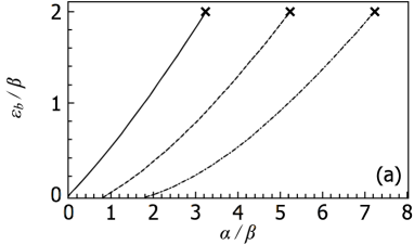
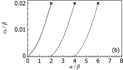
Figure 1: The dependence of the exciton binding energy $\varepsilon_{b}/\beta$ on the interaction strength: (a) - for a semiconductor nanotube with $\Delta/\beta=1$; (b) - for a quasi-metallic nanotube with $\Delta/\beta=0.01$. The different lines correspond to different excitonic states. The crosses indicate the exact analytic results for zero-energy states ($\varepsilon_{b}=\varepsilon_{g}$).

Note also, that by reducing Eq. (4) for $\varepsilon=0$ to the hypergeometric equation (see Appendix B) one can find the analytical expression for the values of the parameter $\alpha/\beta$ when the exciton binding energy is exactly equal to the bandgap:

$$\frac{\alpha}{\beta}=1+2n+\sqrt{1+4\frac{\Delta^{2}}{\beta^{2}}},$$ (6)

where $n=0,1,2,...\;$. These exact values are shown by the crosses in Fig. 1.

It is convenient to express the dimensionless interaction strength $\alpha/\beta$ as

$$\frac{\alpha}{\beta}=\frac{e^{2}}{\epsilon d\hbar v_{\textrm{\scriptsize{F}}}\beta}=\frac{c}{v_{\textrm{\scriptsize{F}}}}\frac{e^{2}}{\hbar c}\frac{1}{\epsilon\beta d}\approx\frac{300}{137}\frac{1}{\epsilon\beta d}.$$ (7)

When the interaction strength is written in the above form, one can immediately see the direct relation of the strongly-bound exciton problem to the long-standing problem of a supercritical charge (the nuclear charge with $Z>137$) and atomic collapse in relativistic quantum mechanics Zeldovich71 . This problem has recently been revisited and reformulated for graphene ShytovSSC09 where the effective impurity charge is increased by a factor of $c/v_{\textrm{\scriptsize{F}}}\approx 300$, which is also present in the numerator of Eq. (7). It follows from Eq. (6) that for an exciton in a narrow-gap carbon nanotube ($\Delta\ll\beta$) the effective supercritical charge corresponding to $\varepsilon_{b}>\varepsilon_{g}$ can be achieved for $\alpha/\beta>2$. In principle, parameters $\epsilon$ and $\beta$ can be controlled by submerging nanotubes in a solution or changing the number of electrons and holes by injection, optical excitation or varying temperature. However, one should not expect the value of $1/(\epsilon\beta d)$ to be higher for a quasi-metallic carbon nanotube than for a semiconductor nanotube of similar diameter.

Fig. 2 shows the dependence of the ratio of the binding energy of the 1s exciton to the value of the gap on the interaction strength for the cases of the semiconductor and narrow gap nanotubes. For very small interaction strengths the ratio $\varepsilon_{b}/\varepsilon_{g}$ is a universal quadratic function of $\alpha/\beta$ (see Appendix C). The two curves remain practically indistinguishable from one another with increasing $\alpha/\beta$ up to $\alpha/\beta\approx 0.6$. A further increase of the interaction strength or range leads to the breakdown of universality for finite range potentials.

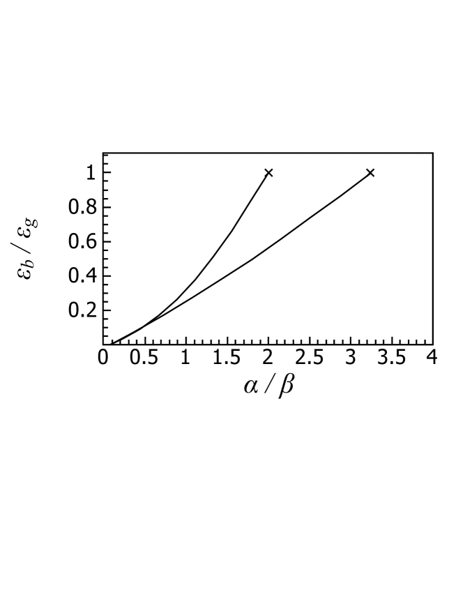
Figure 2: The dependence of the ratio of the exciton binding energy to the nanotube band gap on the interaction strength for a quasi-metallic carbon nanotube with $\Delta/\beta=0.01$ (upper curve) and a semiconductor nanotube with $\Delta/\beta=1$. Only s-states are shown. The crosses correspond to the exact analytic results when the exciton binding energy is equal to the band gap.

It should be noted, that for a zero-range attractive potential between the electron and hole Roemer09 this universality holds for the whole range of interaction strength (see Appendix D). However, for the smooth interaction potential considered here the universality breaks for sufficiently large interaction strength. The difference between the case of semiconductor and quasi-metallic nanotubes is not as large as one could expected. Namely, the value of $\alpha/\beta$ for which the 1s-exciton binding energy is exactly equal to the band gap is about 3.2 for the case of a semiconductor nanotube with $\Delta/\beta=1$ and about 2 for a quasi-metallic nanotube with $\Delta/\beta=0.01$. Also, the variational calculations Pedersen of the binding energy in semiconductor nanotubes supported by the experimental data gives a value for the exciton binding energy of approximately 30 percent of the bandgap which according to Fig. 2 corresponds to the values of $\alpha/\beta\approx 1$. Using the experimental data for the exciton binding energy for the excited subbands of metallic tubes Shaver1 provides even smaller values for $\alpha/\beta$. These estimations ensure that for a quasi-metallic nanotube the 1s exciton bound state lies within the gap. The hypothetical situation $\alpha/\beta>2$ corresponds to the case of the so-called “excitonic insulator”, Jerome where the account of many body effects becomes crucially important and goes beyond the scope of our consideration, which is essentially a two-particle approach. Certain many-body aspects of the physics of excitons in narrow gap nanotubes and their relation to the Luttinger liquid model have been recently studied using a numerical renormalization group.Konik10

Fig. 3 shows the square modulus of the excitonic wavefunction in real space for a quasi-metallic nanotube. One sees that for the 1s state the density in the center of mass has a local minimum, which differs strikingly from the result obtained earlier for semiconductor nanotubes in the effective-mass approximation,WangScience05 in which the probability density in the exciton center of mass has a maximum. This is related to the complex matrix structure of the Hamiltonian (1) resulting in the multi-component structure of the eigenfunctions. A similar dip in the ground-state density was previously reported for graphene-based waveguides.Richard

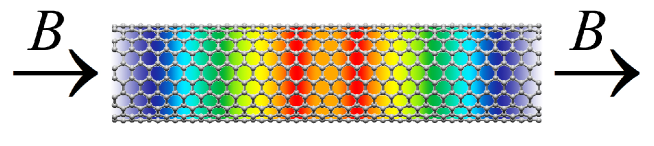
Figure 3: (Color on-line) The density of the 1s-exciton for a (10,10) carbon nanotube with a magnetic field induced gap of $10\;$meV ($2.5\;$THz) corresponding to a magnetic field of $15\;$T along the nanotube axis. The density represents the probability of finding the electron and hole comprising the exciton at the indicated relative separation. Red and blue colors correspond to the highest and lowest values of density, respectively.

It should be noted that taking into account the valley and spin quantum numbers increases the number of different types of excitons associated with a given carbon nanotube spectrum branch to sixteen.AndoReview09 Their consideration, however, can be done along the lines described above, the only difference being the modified interaction strength $\alpha/\beta$ for each type of exciton. The exciton with the highest binding energy in a semiconductor nanotube is known to be optically inactive (dark). The difference between the energy of the dark and bright excitons is proportional to the exciton binding energy and exceeds $k_{\textrm{\scriptsize{B}}}T$ at room temperature causing a significant suppression in the optical emission from semiconductor nanotubes. As it is shown above, for narrow-gap nanotubes the binding energy is drastically reduced and there should be no noticeable difference in the population of dark and bright excitonic states at any experimentally attainable temperatures. At room temperature, all dark and bright excitons in narrow-gap nanotubes should be fully ionized and the direct inter-band transitions PortnoiNano ; PortnoiSM ; PortnoiJMPB govern the emission in the terahertz range.

IV Conclusions

In conclusion, we considered the formation of the exciton in narrow gap carbon nanotubes characterized by the quasi-relativistic spectrum of free particles. We show that the exciton binding energy scales with the band gap and vanishes with decreasing the gap even for strong electron-hole attraction. Therefore, excitonic effects including strongly-bound dark excitons, which explain the poor electroluminescent properties of semiconducting nanotubes, should not dominate for narrow-gap carbon nanotubes. This opens the possibility of using quasi-metallic carbon nanotubes for various terahertz applications.

Appendix A Armchair carbon nanotube in a magnetic field

Graphene’s effective matrix Hamiltonian following the notations of Ref. Saito, is given by

$$H=t\left(\begin{array}[]{cc}0&f_{k}\\ f_{k}^{\star}&0\end{array}\right)$$

and the corresponding eigenvalues are

$$E=\pm\left|t\right|\sqrt{\left|f_{k}\right|^{2}},$$

where

$$f_{k}=\exp\left(i\frac{a}{\sqrt{3}}k_{x}\right)+2\exp\left(-i\frac{a}{2\sqrt{3}}k_{x}\right)\cos\left(k_{y}\frac{a}{2}\right).$$ (8)

For an $\left(n,n\right)$ armchair carbon nanotube, $k_{x}$ is quantized in the following manner

$$k_{x}=\frac{2\pi}{a\sqrt{3}}\frac{l}{n},$$

where $l$ is an integer. Defining $k_{T}$ as the projection of the wavevector along the nanotube axis Eq. (8) can be expressed as

$$f_{k}=\exp\left(i\frac{2\pi}{3}\frac{l}{n}\right)+2\exp\left(-i\frac{\pi}{3}\frac{l}{n}\right)\cos\left(\frac{k_{T}a}{2}\right).$$ (9)

In the presence of a magnetic field, $l\rightarrow l+\mathcal{F}$ (here $\mathcal{F}=\Phi/\Phi_{0}$) and the armchair carbon nanotube energy spectrum becomes

$$E=\pm\left|t\right|\sqrt{1+4\cos\left(\pi\frac{l+\mathcal{F}}{n}\right)\cos\left(\frac{k_{T}a}{2}\right)+4\cos^{2}\left(\frac{k_{T}a}{2}\right)}.$$ (10)

We are interested solely in the lowest conduction and highest valence subbands, which correspond to $l=n$. In this instance the subbands energy spectra are

$$E=\pm\left|t\right|\sqrt{1-4\cos\left(\pi\frac{\mathcal{F}}{n}\right)\cos\left(\frac{k_{T}a}{2}\right)+4\cos^{2}\left(\frac{k_{T}a}{2}\right)},$$ (11)

where the $+\,\left(-\right)$ sign denotes the lowest conduction (highest valence) subband. The introduction of a magnetic field along the nanotube axis shifts the minimum in the spectrum away from $k_{T}=2\pi/3a$, the electrons “acquire mass” and a band gap is opened. The new minimum, $k_{T}^{\mathrm{min}}$, is obtained by differentiating Eq.(11) and equating it to zero, this yields:

$$\frac{1}{2}\cos\left(\pi\frac{\mathcal{F}}{n}\right)=\cos\left(k_{T}^{\mathrm{min}}\frac{a}{2}\right).$$ (12)

Since we are interested in particle behavior in the vicinity of $k_{T}^{\mathrm{min}}$, it is natural to re-express the electron energy spectrum in terms of $q_{T}$, defined as the momentum measured relative to $k_{T}^{\mathrm{min}}$ i.e. $k_{T}=k_{T}^{\mathrm{min}}+q_{T}$, thus Eq. (9) can be expressed by

$$f_{k}=\exp\left[-i\frac{\pi}{3}\left(1+\frac{\mathcal{F}}{n}\right)\right]\left\{-\exp\left(i\pi\frac{\mathcal{F}}{n}\right)+2\cos\left[\left(k_{T}^{min}+q_{T}\right)\frac{a}{2}\right]\right\}.$$

Using the identity Eq. (12) $f_{k}$ becomes:

$$f_{k}=\exp\left[-i\frac{\pi}{3}\left(1+\frac{\mathcal{F}}{n}\right)\right]\left[\cos\left(\pi\frac{\mathcal{F}}{n}\right)\cos\left(\frac{aq_{T}}{2}\right)-2\sqrt{1-\frac{1}{4}\cos^{2}\left(\pi\frac{\mathcal{F}}{n}\right)}\sin\left(\frac{aq_{T}}{2}\right)-\exp\left(i\pi\frac{\mathcal{F}}{n}\right)\right].$$ (13)

Expanding Eq. (13) in terms of $q_{T}$ and retaining first order terms only yields

$$f_{k}=\exp\left[-i\frac{\pi}{3}\left(1+\frac{\mathcal{F}}{n}\right)\right]\left(-i\sin\left(\pi\frac{\mathcal{F}}{n}\right)-\sqrt{1-\frac{1}{4}\cos^{2}\left(\pi\frac{\mathcal{F}}{n}\right)}aq_{T}\right).$$ (14)

The effective matrix Hamiltonian can therefore be written as:

$$\hat{H}_{0}=t\left(\begin{array}[]{cc}0&e^{-i\theta}\left(-i\sin\left(\pi\frac{\mathcal{F}}{n}\right)-\sqrt{1-\frac{1}{4}\cos^{2}\left(\pi\frac{\mathcal{F}}{n}\right)}a\hat{q}\right)\\ e^{i\theta}\left(i\sin\left(\pi\frac{\mathcal{F}}{n}\right)-\sqrt{1-\frac{1}{4}\cos^{2}\left(\pi\frac{\mathcal{F}}{n}\right)}a\hat{q}\right)&0\end{array}\right),$$ (15)

where $\theta=\frac{\pi}{3}\left(1+\frac{\mathcal{F}}{n}\right)$ and $\hat{q}=-i\frac{\partial}{\partial y}$. This $2\times 2$ Hamiltonian acts on a two-component Dirac wavefunction with components $\chi_{1}$ and $\chi_{2}$ associated with the $A$ and $B$ sublattices of graphene respectively. By changing the basis wavefunctions from $\chi_{1}$ and $\chi_{2}$ to $\psi_{A}=-\chi_{1}$ and $\psi_{B}=-\exp(-i\theta)\chi_{2}$, and changing the variable $y\rightarrow-x$, so that the $x$-coordinate is now along the nanotube axis, the effective matrix Hamiltonian can be expressed as

$$\hat{H}_{0}=\left|t\right|\left(\begin{array}[]{cc}0&\sqrt{1-\frac{1}{4}\cos^{2}\left(\pi\frac{\mathcal{F}}{n}\right)}a\hat{q}-i\sin\left(\pi\frac{\mathcal{F}}{n}\right)\\ \sqrt{1-\frac{1}{4}\cos^{2}\left(\pi\frac{\mathcal{F}}{n}\right)}a\hat{q}+i\sin\left(\pi\frac{\mathcal{F}}{n}\right)&0\end{array}\right),$$ (16)

which acts on the two-component Dirac wavefunction $(\psi_{A},\psi_{B})^{\textrm{T}}$. For brevity let $b=\sqrt{\frac{4}{3}-\frac{1}{3}\cos^{2}\left(\frac{\pi}{n}{\mathcal{F}}\right)}$ and $\Delta=\frac{2}{a\sqrt{3}}\sin\left(\frac{\pi}{n}{\mathcal{F}}\right)$. Thus,

$$\hat{H}_{0}=\hbar v_{\mathrm{F}}\left(\begin{array}[]{cc}0&b\hat{q}-i\Delta\\ b\hat{q}+i\Delta&0\end{array}\right),$$ (17)

where now $\hat{q}=-i\frac{\partial}{\partial x}$.

Appendix B Derivation of the analytic solution for $E=0$

For the case of total momentum $K=0$, corresponding to the static exciton, the multi-component wavefunction of relative motion satisfies the matrix equation given by Eq. (3) of the main text. Since $\phi_{AA}=\phi_{BB}$, the system of equations (3) reduces to

$$\phi_{BA}=\frac{2}{\left[\varepsilon-\tilde{V}\left(x\right)\right]}\left(\hat{k}+i\Delta\right)\phi_{AA};$$ (18)

$$\phi_{AB}=\frac{2}{\left[\varepsilon-\tilde{V}\left(x\right)\right]}\left(\hat{k}-i\Delta\right)\phi_{AA};$$ (19)

$$\left(\hat{k}-i\Delta\right)\phi_{BA}+\left(\hat{k}+i\Delta\right)\phi_{AB}=\left[\varepsilon-\tilde{V}\left(x\right)\right]\phi_{AA}.$$ (20)

Substituting Eq. (18) and Eq. (19) into Eq. (20) yields the following second order differential equation:

$$\frac{d^{2}\phi_{AA}}{dx^{2}}+\frac{1}{\varepsilon-\tilde{V}(x)}\,\frac{d\tilde{V}(x)}{dx}\,\frac{d\phi_{AA}}{dx}+\left[\left(\frac{\varepsilon-\tilde{V}(x)}{2}\right)^{2}-\Delta^{2}\right]\phi_{AA}=0,$$ (21)

which coincides with Eq. (4) of the main text.

Let us now consider the case of

$$\tilde{V}\left(x\right)=-\frac{\alpha}{\cosh\left(\beta x\right)}$$

and $\varepsilon=0$. Making the change of variable $z=\beta x$ transforms Eq. (21) to

$$\frac{d^{2}\phi_{AA}}{dz^{2}}+\tanh\left(z\right)\frac{d\phi_{AA}}{dz}+\left[-\frac{1}{4}\omega^{2}\tanh^{2}\left(z\right)+\frac{1}{4}\omega^{2}-\tilde{\Delta}^{2}\right]\phi_{AA}=0,$$ (22)

where $\omega=\alpha/\beta$ and $\tilde{\Delta}=\Delta/\beta$. The change of variable $\chi=\tanh\left(z\right)$ allows Eq. (22) to be expressed as

$$\left(\chi^{2}-1\right)^{2}\frac{\partial^{2}\phi_{AA}}{\partial\chi^{2}}+\chi\left(\chi^{2}-1\right)\frac{\partial\phi_{AA}}{\partial\chi}+\left(c\chi^{2}+e\right)\phi_{AA}=0,$$ (23)

where $c=-\frac{1}{4}\omega^{2}$ and $e=\frac{1}{4}\omega^{2}-\Delta^{2}$. Eq. (23) is of a known form and has the solutions Kamke_Book

$$\phi_{AA}=A_{1}\left(\chi+1\right)^{p}\left(\chi-1\right)^{q}\eta\left[\frac{1}{2}\left(\chi+1\right)\right],$$ (24)

where $A_{1}$ is a constant, the function $\eta\left[\frac{1}{2}\left(\chi+1\right)\right]$ is to be found and $p$ and $q$ are found from the following conditions:

$$4q\left(q-1\right)+2q+c+e=0;$$

$$\qquad\left(p-q\right)\left[2\left(p+q\right)-1\right]=0.$$ (25)

Eqs. (23, 24, 25) yield

$$\left(\chi^{2}-1\right)\frac{\mathrm{d}^{2}\eta}{\mathrm{d}\chi^{2}}+\left[\left(2p+2q+1\right)\chi-2\left(p-q\right)\right]\frac{\mathrm{d}\eta}{\mathrm{d}\chi}+\left[\left(p+q\right)^{2}+c\right]\eta=0.$$ (26)

Performing a change of variable $\left(\chi+1\right)/2\rightarrow\kappa$ reduces Eq. (26) to the hypergeometric equation

$$\kappa\left(\kappa-1\right)\frac{\mathrm{d}^{2}\eta}{\mathrm{d}\kappa^{2}}+\left[\left(a_{1}+a_{2}+1\right)\kappa-a_{3}\right]\frac{\mathrm{d}\eta}{\mathrm{d}\kappa}+a_{1}a_{2}\eta=0,$$

where $a_{1}=p+q\pm\sqrt{-c}$, $a_{2}=p+q\mp\sqrt{-c}$ and $a_{3}=2p+\frac{1}{2}$. Thus, the form of $\eta$ is

$$\eta=\mathrm{{}_{2}F_{1}}\left(p+q-\sqrt{-c},\,p+q+\sqrt{-c};\,2p+\frac{1}{2};\,\kappa\right).$$ (27)

Hence the wavefunction $\phi_{AA}$ is given by

$$\phi_{AA}=A_{1}\left(1+\chi\right)^{p}\left(1-\chi\right)^{q}\mathrm{{}_{2}F_{1}}\left(p+q-\frac{\omega}{2},\,p+q+\frac{\omega}{2};\,2p+\frac{1}{2};\,\frac{1+\chi}{2}\right).$$ (28)

From Eq. (25) $q$ is found to be

$$q=\frac{1\pm\sqrt{1+4\tilde{\Delta}^{2}}}{4},$$ (29)

and $p$ can take the values

$$p=q$$ (30)

or

$$p=\frac{1}{2}-q.$$ (31)

Let us first consider the case of $p=q$. In this instance Eq. (28) becomes

$$\phi_{AA}=A_{1}\left[1-\chi^{2}\right]^{q}\mathrm{{}_{2}F_{1}}\left(2q-\frac{\omega}{2},\,2q+\frac{\omega}{2};\,2q+\frac{1}{2};\,\frac{1+\chi}{2}\right).$$ (32)

For the function $\phi_{AA}$ to vanish as $z\rightarrow\infty$ we require

$$q=\frac{1\pm\sqrt{1+4\tilde{\Delta}^{2}}}{4}>0$$ (33)

and that the hypergeometric series is terminated. This can be satisfied if we take the positive root of $q$ and restrict $\omega$ such that $2q-\frac{\omega}{2}=-n$, where $n$ is a positive integer, thus we arrive at the condition that

$$\omega=1+2n+\sqrt{1+4\tilde{\Delta}^{2}}.$$ (34)

The functions $\phi_{BA}$ and $\phi_{AB}$, which can be found from Eq. (18) and Eq. (19), must also vanish as $z\rightarrow\infty$. For simplicity let us analyze the linear combinations $\Psi_{+}=\phi_{BA}+\phi_{AB}$ and $\Psi_{-}=\phi_{BA}-\phi_{AB}$:

$$\Psi_{+}=i\frac{4\beta}{V\left(z\right)}\frac{\partial\phi_{AA}}{\partial z}=-i\frac{4}{\omega}\cosh\left(z\right)\frac{\partial\phi_{AA}}{\partial z};$$ (35)

$$\Psi_{-}=-i\frac{4\Delta}{V\left(z\right)}\phi_{AA}=i\frac{4\tilde{\Delta}}{\omega}\cosh\left(z\right)\phi_{AA}.$$ (36)

For the functions satisfying Eqs. (35) and (36) to vanish in the limit of $z\rightarrow\infty$, we require

$$q=\frac{1+\sqrt{1+4\tilde{\Delta}^{2}}}{4}>\frac{1}{2}.$$ (37)

This is automatically satisfied for any finite $\tilde{\Delta}$. Therefore, providing $\phi_{AA}$ vanishes as $z\rightarrow\infty$, $\phi_{BA}$ and $\phi_{AB}$ will also vanish.

Let us now consider the case of $p+q=\frac{1}{2}$, in this instance Eq. (28) becomes

$$\phi_{AA}=\tilde{A}_{1}\left(1-\chi^{2}\right)^{q}\left(1+\chi\right)^{\frac{1}{2}-2q}\mathrm{{}_{2}F_{1}}\left(\frac{1}{2}-\frac{\omega}{2},\,\frac{1}{2}+\frac{\omega}{2};\,\frac{3}{2}-2q;\,\frac{1+\chi}{2}\right).$$ (38)

Using the identity Abramowitz_Stegun

$$z^{1-c}\mathrm{{}_{2}F_{1}}\left(a+1-c,\,b+1-c;\,2-c;\,z\right)=\mathrm{{}_{2}F_{1}}\left(a,\,b;\,c;\,z\right),$$ (39)

where $a=2q-\frac{\omega}{2}$, $b=2q+\frac{\omega}{2}$, $c=2q+\frac{1}{2}$ and $z=\left(1+\chi\right)/2$, Eq. (38) becomes

$$\phi_{AA}=\tilde{A}_{2}\left[1-\chi^{2}\right]^{q}\mathrm{{}_{2}F_{1}}\left(2q-\frac{\omega}{2},\,2q+\frac{\omega}{2};\,2q+\frac{1}{2};\,\frac{1+\chi}{2}\right),$$ (40)

where $\tilde{A}_{2}$ is a constant. This is of the same form as Eq. (32).

Appendix C Binding energy in the limit of weak electron-hole attraction

Let us consider the limit of very weak electron-hole attraction: $|\tilde{V}(x)|\ll\Delta$ for any inter-particle separation. Substituting $\varepsilon=2\Delta-\varepsilon_{b}$ into Eq. (4) and retaining only the first order terms in $\tilde{V}/\Delta$ and $\varepsilon_{b}/\Delta$ transforms Eq. (4) into

$$-\frac{1}{\Delta}\frac{d^{2}\phi_{AA}}{dx^{2}}+\tilde{V}(x)\,\phi_{AA}=-\varepsilon_{b}\phi_{AA}.$$ (41)

Eq. (41) is of the form of the non-relativistic one-dimensional Schrödinger equation, where the parameter $\Delta$, plays the role of the effective mass. For a particle of mass $m$ in a weak one-dimensional potential $U(x)$, the textbookLandau treatment of the potential as a perturbation yields the following result for the binding energy: $|E|=(m/2\hbar^{2})\left[\int_{-\infty}^{\infty}U(x)dx\right]^{2}$, which can be reformulated for Eq. (41) as

$$\varepsilon_{b}=\frac{\Delta}{4}\left[\int_{-\infty}^{\infty}\tilde{V}(x)dx\right]^{2}.$$ (42)

For $\tilde{V}(x)=-\alpha/\cosh(\beta x)$, Eq. (42) yields

$$\varepsilon_{b}=\frac{\pi^{2}}{4}\Delta\,\left(\alpha/\beta\right)^{2}.$$ (43)

Thus, we have shown that for a weak hyperbolic secant potential, when $\alpha\ll\Delta$, the binding energy scales with the band gap and has the universal quadratic dependence on $\alpha/\beta$. Notably, Eq. (43) is also true for a weak interaction potential given by a Lorentzian, $\tilde{V}(x)=\alpha/\left(1+\beta^{2}x^{2}\right)$.

Appendix D Exciton with attractive delta-function potential

The problem of calculating the energy of an exciton in a carbon nanotube can be solved exactly in the case when interaction potential between the electron and hole is taken to be a delta-function, $\tilde{V}(x)=-U_{0}\delta(x)$, where the strength of the potential $U_{0}$ is positive and can be estimated as a product of the strength of the realistic potential and its width.

Let us consider an electron-hole pair in a narrow-gap 1D carbon nanotube with a band gap energy of $4|\Delta|$. Measuring all quantities in units of $\hbar v_{F}$ as above, one can write the Hamiltonian as

$$\widehat{H}=\sqrt{\Delta^{2}+\widehat{q}_{e}^{2}}+\sqrt{\Delta^{2}+\widehat{q}_{h}^{2}}+\tilde{V}(|x_{e}-x_{h}|),$$ (44)

where

$$\widehat{q}_{e,h}=-i\frac{\partial}{\partial x_{e,h}}.$$ (45)

Here we have retained only the eigenstates of the general graphene-type Hamiltonian with positive energies. The Schrodinger equation for the problem we consider thus reads

$$\left[\sqrt{\Delta^{2}+\widehat{q}_{e}^{2}}+\sqrt{\Delta^{2}+\widehat{q}_{h}^{2}}+\tilde{V}(|x_{e}-x_{h}|)\right]\Psi(x_{e},x_{h})=\varepsilon\Psi(x_{e},x_{h}).$$ (46)

Introducing new variables corresponding to the center of mass and relative motion in the manner explained in the text of the article and putting the wavevector of the center of mass motion equal to zero, one gets the following expression

$$2\sqrt{\Delta^{2}-\frac{d^{2}}{dx^{2}}}\psi(x)=\left[\varepsilon-\tilde{V}(x)\right]\psi(x),$$ (47)

where $\psi(x)$ is a wavefunction of relative motion. The above expression is a 1D Schrödinger equation for a particle with a complicated dispersion placed in an external potential $\widetilde{V}(x)$, which can be solved for the case when $\tilde{V}(x)=-U_{0}\delta(x)$. Indeed, in this case the solution of the Schrödinger equation corresponding to a bound state reads

$$\psi(x)=Ae^{\kappa(\epsilon)x},~{}x<0,$$ (48)

$$\psi(x)=Ae^{-\kappa(\epsilon)x},~{}x>0,$$ (49)

where $\varepsilon=2\sqrt{\Delta^{2}+\kappa^{2}}$. It is well known that the zero-range delta potential is equivalent to the introduction of the specific boundary condition for the derivative of the solution at $x=0$ (the function itself should be continuous, $\psi(+0)=\psi(-0)$). To obtain a condition for the derivative, let us integrate the Schrödinger equation

$$\left[\widehat{H}_{0}\left(\frac{d}{dx}\right)-\varepsilon\right]\psi(x)=U_{0}\delta(x)\psi(x),$$ (50)

where $\widehat{H}_{0}\left(\frac{d}{dx}\right)=2\sqrt{\Delta^{2}+\frac{d^{2}}{dx^{2}}}$ across the interval $[-0;+0]$; this yields

$$\int{\widehat{H}_{0}\left(\frac{d}{dx}\right)\psi(x)dx}|_{x=+0}-\int{\widehat{H}_{0}\left(\frac{d}{dx}\right)\psi(x)dx}|_{x=-0}=U_{0}\psi(0).$$ (51)

Using this relation and Eqs. (48), (49) and (47) one gets the following expression for determining the parameter $\kappa$

$$H_{0}(-\kappa)+H_{0}(\kappa)-2H_{0}(0)=-\kappa U_{0}.$$ (52)

Thus,

$$\sqrt{\Delta^{2}-\kappa^{2}}=\Delta-\frac{\kappa U_{0}}{4},$$ (53)

which yields

$$\kappa=\frac{8U_{0}\Delta}{16+U_{0}^{2}},$$ (54)

where the energy is given by

$$\varepsilon=2\sqrt{\Delta^{2}-\kappa^{2}}.$$ (55)

Note, that this result is valid only for the case of $U_{0}<4$, as for $U_{0}>4$, the right hand side of Eq. (53) is negative. The binding energy of the exciton can be determined as

$$\varepsilon_{b}=2\Delta-\epsilon=4\Delta U_{0}^{2}/(16+U_{0}^{2}),$$ (56)

which tends to the non-relativistic result of $\varepsilon_{b}=U_{0}^{2}\Delta/4$ for $U_{0}\ll 1$; c.f. this result with Eq. (42). Note, that in both relativistic and non-relativistic cases the binding energy is proportional to the gap.

References

- (1) P. R. Wallace, Phys. Rev. 71, 622 (1947)
- (2) K. S. Novoselov, A. K. Geim, S. V. Morozov, D. Jiang, M. I. Katsnelson, I. V. Grigorieva, S. V. Dubonos, and A. A. Firsov, Nature (London) 438, 197 (2005).
- (3) See, e.g., a review article A. H. Castro Neto, F. Guinea, N. M. R. Peres, K. S. Novoselov, and A. K. Geim, Rev. Mod. Phys. 81, 109 (2009).
- (4) J.-C. Charlier, X. Blase, and S. Roche, Rev. Mod. Phys. 79, 677 (2007).
- (5) R. Saito, G. Dresselhaus, and M. S. Dresselhaus, Physical Properties of Carbon Nanotubes (Imperial College Press, London, 1998).
- (6) H. Ajiki and T. Ando, J. Phys. Soc. Jpn. 62, 1255 (1993).
- (7) S. M. Bachilo, M. S. Strano, C. Kittrell, R. H. Hauge, R. E. Smalley, and R. B. Weisman, Science 298, 2361 (2002).
- (8) A. Hartschuh, H. N. Pedrosa, L. Novotny, and T. D. Krauss, Science 301, 1354 (2003).
- (9) F. Wang, G. Dukovic, L. E. Brus, and T. F. Heinz, Phys. Rev. Lett. 92, 177401 (2004).
- (10) F. Wang, G. Dukovic, L. E. Brus, and T. F. Heinz, Science 308, 838 (2005).
- (11) S. Berciaud, L. Cognet and B. Lounis, Phys. Rev. Lett. 101, 077402 (2008).
- (12) J. Shaver, J. Kono, O. Portugall, V. Krstic, G. L. J. A. Rikken, Y. Miyauchi, S. Maruyama, and V. Perebeinos, Nano Lett. 7, 1851 (2007).
- (13) J. Shaver, J. Kono, Laser & Photon. Rev. 1, 260 (2007) and references therein.
- (14) A. D. Mohite, P. Gopinath, H. M. Shah, B. W. Alphenaar, Nano Lett. 8, 142 (2008).
- (15) T. G. Pedersen, Carbon 42, 1007 (2004).
- (16) V. Perebeinos, J. Tersoff, P. Avouris, Phys. Rev. Lett. 92, 257402 (2004).
- (17) S. Uryu and T. Ando, Phys. Rev. B 76, 115420 (2007).
- (18) For a review see T. Ando and S. Uryu, Phys. Status Solidi C 6, 173 (2009).
- (19) J. Deslippe, C. D. Spataru, D. Prendergast, S. G. Louie, Nano Lett. 7, 1626 (2007).
- (20) E. Malic, J. Maultzsch, S. Reich, and A. Knorr, Phys. Rev. B 82, 035433 (2010).
- (21) O. V. Kibis, M. Rosenau da Costa, and M. E. Portnoi, Nano Lett. 7, 3414 (2007).
- (22) M. E. Portnoi, O. V. Kibis, M. Rosenau da Costa, Superlattices Microstruct. 43, 399 (2008).
- (23) M. E. Portnoi, M. Rosenau da Costa, O. V. Kibis, and I. A. Shelykh, Int. Journ. Mod. Phys. B 23, 2846 (2009).
- (24) T. Ando, J. Phys. Soc. Jpn. 66, 1066 (1997)
- (25) D. Jerome, T. M. Rice, and W. Kohn, Phys. Rev. 158, 462 (1967).
- (26) C. L. Kane and E. J. Mele, Phys. Rev. Lett. 78, 1932 (1997).
- (27) L. Brey and H. A. Fertig, Phys. Rev. B 73, 235411 (2006).
- (28) R. R. Hartmann, N. J. Robinson, and M. E. Portnoi, Phys. Rev. B 81, 245431 (2010).
- (29) Y. B. Zeldovich, V. S. Popov, Usp. Fiz. Nauk 105, 403 (1971); Sov. Phys. Usp. 14, 673 (1972).
- (30) A. Shytov, M. Rudner, N. Gu, M. Katsnelson, and L. Levitov, Solid State Commun. 149 1087 (2009).
- (31) A. M. Fischer, V. L. Campo, Jr., M. E. Portnoi, and R. A. Römer, Phys. Rev. Lett. 102, 096405 (2009).
- (32) R. M. Konik, arXiv:1007.4773; Phys. Rev. Lett. 106, 136805 (2011).
- (33) E. Kamke, Differentialgleichungen - Lösungsmethoden und Lösungen (Chelsea Publishing Company, New York, 1974).
- (34) M. Abramowitz, I. A. Stegun, Handbook of Mathematical Functions with Formulas, Graphs, and Mathematical Tables (Dover Publications, New York, 1972).
- (35) L. D. Landau and E. M. Lifshitz, Quantum Mechanics: Non-Relativistic Theory (Pergamon Press, Oxford, 1991), p.163.