Role of different model ingredients in the exotic cluster-decay of ⁵⁶Ni^∗
Narinder K. Dhiman
Govt. Sr. Sec. School, Summer Hill, Shimla -171005, India

We present cluster decay studies of ⁵⁶Ni^∗ formed in heavy-ion collisions using different Fermi density and nuclear radius parameters proposed by various authors. Our study reveals that different technical parameters do not alter the transfer structure of fractional yields significantly. The cluster decay half-lives of different clusters lies within $\pm$10% for different Fermi density parameters and nuclear radius, therefore, justify the current set of parameters used in the literature for the calculations of cluster decay.

1 Introduction

In earlier days, nucleus was considered to have a uniform density and sharp radius. With the passage of time, the density distribution was found to be more complicated. Several different forms (direct or indirect) exist in literature that can explain these complicated nuclear density distributions. The first method is the direct parametrization which involves the choice of a suitable functional form where parameters are varied to fit the experimental data. The two parameter Fermi density distribution is an example of such a parametrization. The second method is of indirect parametrization of density distribution proceeds via nuclear models. The nuclear models like shell model contains certain parameters which are determined by other physical considerations and it is then used to calculate the nuclear density distribution without further adjustments. The experimental data can be described accurately with two-parameter Fermi density distribution at relatively low momentum. Among all the density distributions two-parameters Fermi density has been quite successful in the low, medium and heavy mass regions. The systematic study of charge distributions have been carried out in Refs.[1, 2, 3]. We shall use this density distribution here.

Since the nuclear systems obey quantum laws, therefore, their surfaces are not well defined. The nuclear density remains constant up to certain distance but fall more rapidly close to the surface region where the nucleons are free to move about. The nuclear densities provide important information about the structure of nuclear matter at low energies and other important information regarding the equation of state at intermediate energies [4, 5].

Various methods have been developed for exploring the nuclear structure and radius. The electron scattering/ electrically charged particles of high energy are employed as probe to explore the proton distribution of the nuclei (i.e charge radii), whereas neutral nuclear probes such as neutrons will give the effect of nuclear forces over the nuclear surface (i.e. interaction radii). The charge radii are often used to extract the information about nuclear radii. The electron scattering experiments shows that the charge distribution within a nucleus either follow Fermi trapezoidal shape or modified Gaussian distribution. These studies have shown that nuclear charge density does not decrease abruptly but has a finite diffuseness.

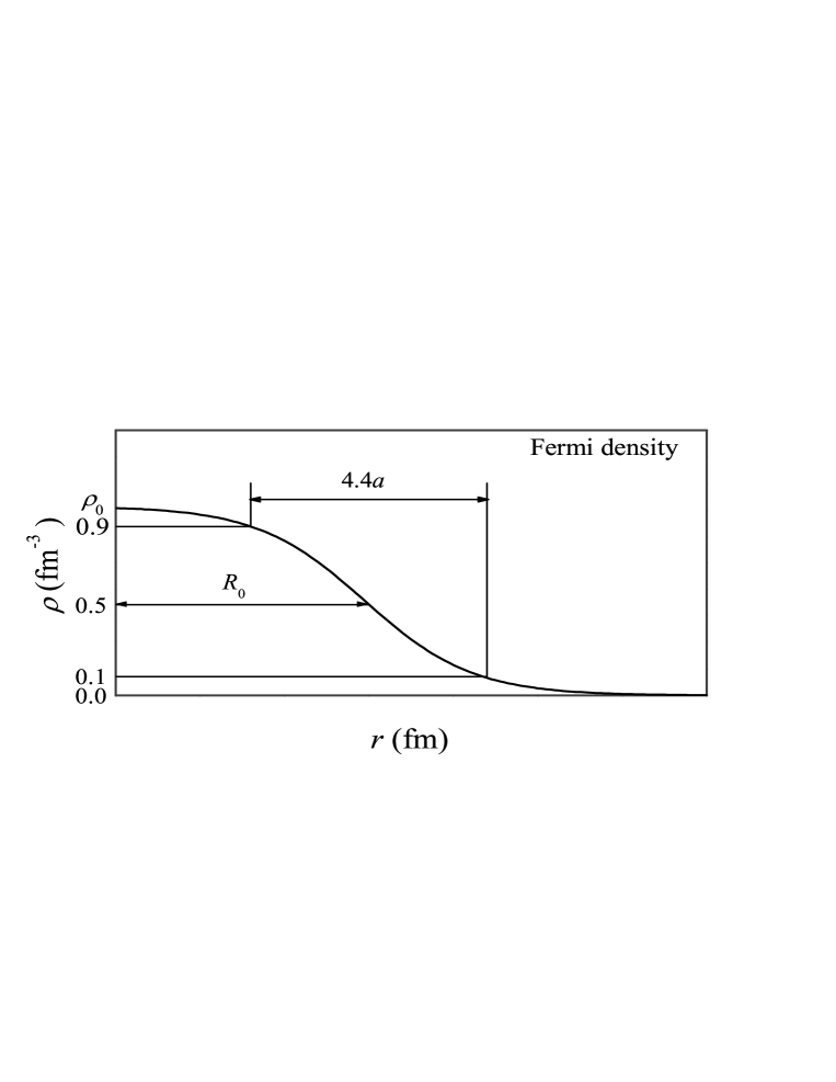
Figure 1: The systematics diagram for two parameter Fermi density.

A model that uses density distribution such as two parameter Fermi density (as shown in Fig. 1) has to rely on the information about nuclear radius (or half density radii $R_{0}$), central density $\rho_{0}$, and surface diffuseness ($a$). Interestingly, several different experimental as well as theoretical values of these parameters are available in literature [6, 7, 8, 9, 10, 11]. In addition, several different names such as central radii, equivalent sharp radii, root mean square radii etc. have also been used in the literature to define different functional forms. The role of different radii was examined in exotic cluster decay half-lives [12] and interestingly two different forms of radii were found to predict five order of magnitude different half-lives within the same theoretical model. Similarly, the use of different values of surface diffuseness also varies from author to author. The effect of these model ingredients on the fusion process at low incident energy have been studied in Ref. [13] and there was found that the effect of different radii is more than marginal and therefore this parameter should be used with a more fundamental basis. Unfortunately, no systematic study is still available in the cluster decay process. In this paper, we plan to study the role of Fermi density parameters in the cluster decay of ⁵⁶Ni^∗ when formed in heavy-ion collisions. This study is still missing in the literature.

Heavy-ion reactions provide a very good tool to probe the nucleus theoretically. This includes low energy fusion process [14], intermediate energy phenomena [15] as well as cluster-decay and/or formation of super heavy nuclei [16, 17]. In the last one decade, several theoretical models have been employed in the literature to estimate the half-life times of various exotic cluster decays of radioactive nuclei. These outcome have also been compared with experimental data. Among all the models employed preformed cluster model (PCM) [18, 19, 20] is widely used to study the exotic cluster decay. In this model the clusters/ fragments are assumed to be pre-born well before the penetration of the barrier. This is in contrast to the unified fission models (UFM) [21, 22, 23], where only barrier penetration probabilities are taken into account. In either of these approach, one needs complete knowledge of nuclear radii and densities in the potential.

Cluster decay of ⁵⁶Ni is studied when formed as an excited compound system in heavy-ion reactions. Since ⁵⁶Ni has negative $Q$-value (or $Q_{out}$) and is stable against both fission and cluster decay processes. However, if is is produced in heavy-ion reactions depending on the incident energy and angular momentum involved, the excited compound system could either fission, decay via cluster emissions or results in resonance phenomenon. The ⁵⁶Ni has a negative $Q_{out}$ having different values for various exit channels and hence would decay only if it were produced with sufficient compound nucleus excitation energy $E^{\ast}_{CN}~{}(=E_{cm}+Q_{in})$, to compensate for negative $Q_{out}$, the deformation energy of the fragments $E_{d}$, their total kinetic energy ($TKE$) and the total excitation energy ($TXE$), in the exit channel as:

$$E^{\ast}_{CN}=\mid Q_{out}\mid+E_{d}+TKE+TXE.$$ (1)

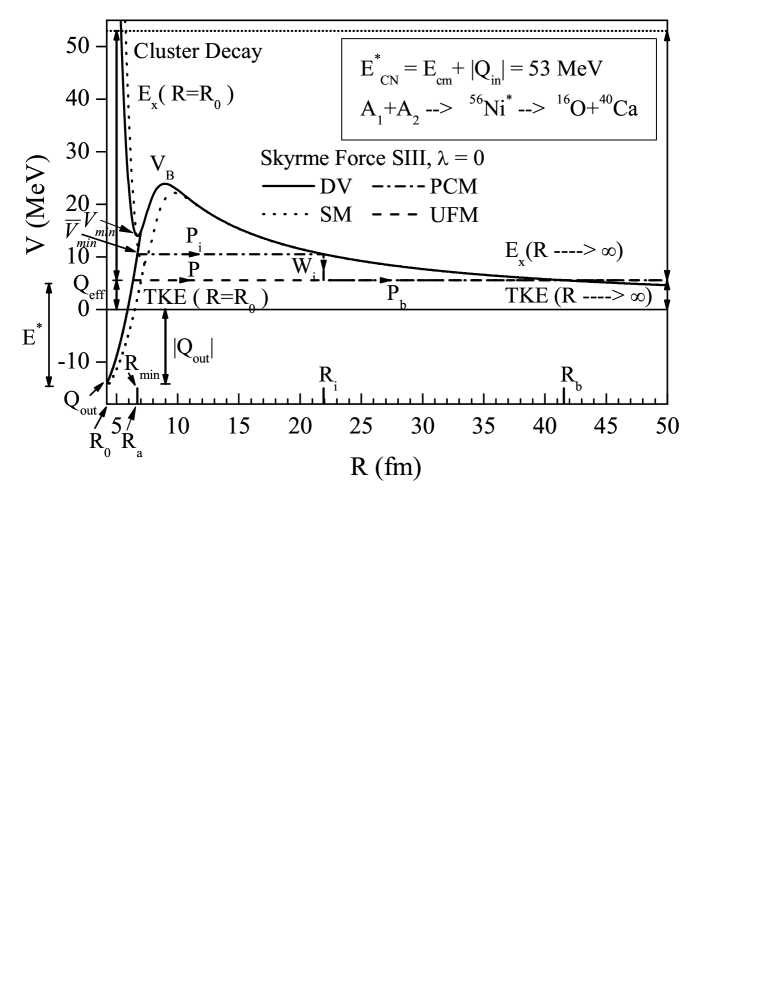
Figure 2: The scattering potential $V(R)$ (MeV) for cluster decay of ⁵⁶Ni^∗ into ¹⁶O + ⁴⁰Ca channel for different Fermi density parameters. The distribution of compound nucleus excitation energy E${}_{CN}^{*}$ at both the initial ($R=R_{0}$) and asymptotic ($R\to\infty$) stages and $Q$-values are shown. The decay path for both PCM and UFM models is also displayed.

(see Fig. 2, where $E_{d}$ is neglected because the fragments are considered to be spherical). Here $Q_{in}$ adds to the entrance channel kinetic energy $E_{cm}$ of the incoming nuclei in their ground states.

Section 2 gives some details of the Skyrme energy density model and preformed cluster model and its simplification to unified fission model. Our calculations for the decay half-life times of ⁵⁶Ni compound system and a discussion of the results are presented in Section 3. Finally, the results are summarized in Section 4.

2 Model

2.1 Skyrme Energy Density Model

In the Skyrme Energy Density Model (SEDM) [7], the nuclear potential is calculated as a difference of energy expectation value $E$ of the colliding nuclei at a finite distance $R$ and at complete isolation (i.e. at $\infty$) [7, 24].

$$V_{N}(R)=E(R)-E(\infty),$$ (2)

where $E=\int H(\vec{r})\vec{dr}$, with $H(\vec{r})$ as the Skyrme Hamiltonian density which reads as:

$$H(\rho,\tau,\vec{J}) = \frac{\hbar^{2}}{2m}\tau+\frac{1}{2}t_{0}[(1+\frac{1}{2}x_{0})\rho^{2}-(x_{0}+\frac{1}{2})(\rho_{n}^{2}+\rho_{p}^{2})]$$ (3)

$$+\frac{1}{4}(t_{1}+t_{2})\rho\tau+\frac{1}{8}(t_{2}-t_{1})(\rho_{n}\tau_{n}+\rho_{p}\tau_{p})$$

$$+\frac{1}{16}(t_{2}-3t_{1})\rho\nabla^{2}\rho+\frac{1}{4}t_{3}\rho_{n}\rho_{p}\rho$$

$$+\frac{1}{32}(3t_{1}+t_{2})(\rho_{n}\nabla^{2}\rho_{n}+\rho_{p}\nabla^{2}\rho_{p})$$

$$-\frac{1}{2}W_{0}(\rho\vec{\nabla}\cdot\vec{J}+\rho_{n}\vec{\nabla}\cdot\vec{J}_{n}+\rho_{p}\vec{\nabla}\cdot\vec{J}_{p}).$$

Here $\vec{J}=\vec{J}_{n}+\vec{J}_{p}$ is the spin density which was generalized by Puri et al. [7], for spin-unsaturated nuclei and $\tau=\tau_{n}+\tau_{p}$ is the kinetic energy density calculated using Thomas Fermi approximation [25, 26], which reduces the dependence of energy density $H(\rho,\tau,\vec{J})$ to be a function of nucleon density $\rho$ and spin density $\vec{J}$ only. Here strength of surface correction factor is taken to be zero (i.e. $\lambda=0$). The remaining term is the nucleon density $\rho=\rho_{n}+\rho_{p}$ is taken to be well known two-parameter Fermi density. The Coulomb effects are neglected in the above energy density functional, but will be added explicitly. In Eq. (3), six parameters $t_{0}$, $t_{1}$, $t_{2}$, $t_{3}$, $x_{0}$, and $W_{0}$ are fitted by different authors to obtain the best description of the various ground state properties for a large number of nuclei. These different parameterizations have been labeled as S, SI, SII, SIII etc. and known as Skyrme forces for light and medium colliding nuclei. Other Skyrme forces are able to reproduce the data for heavy systems better. The Skyrme force used for the present study is SIII with parameters as: $t_{0}=-1128.75$ MeVfm³, $t_{1}=395.00$ MeVfm⁵, $t_{2}=-95.00$ MeVfm⁵, $t_{3}=14000.00$ MeVfm⁶, $x_{0}=0.45$, and $W_{0}=120.00$ MeVfm⁵. It has been shown in previous studies that SIII force reproduces the fusion barrier much better than other sets of Skyrme forces for light and medium nuclei. Other Skyrme forces such as SKa, SKm, however, are found to be better for heavier masses.

From Eq. (3), one observes that the Hamiltonian density $H(\rho,\tau,\vec{J})$ can be divided into two parts: (i) the spin-independent part $V_{P}(R)$, and (ii) spin-dependent $V_{J}(R)$ [7] as:

$$V_{N}(R) = \int\left\{H(\rho)-\left[H_{1}(\rho_{1})+H_{2}(\rho_{2})\right]\right\}d\vec{r}$$ (4)

$$+ \int\left\{H(\rho,\vec{J})-\left[H_{1}(\rho_{1},\vec{J}_{1})+H_{2}(\rho_{2},\vec{J}_{2})\right]\right\}d\vec{r}$$

$$= V_{P}(R)+V_{J}(R)$$

We apply the standard Fermi mass density distribution for nucleonic density:

$$\rho(R)=\frac{\rho_{0}}{1+\exp\left\{\frac{R-R_{0}}{a}\right\}},~{}~{}~{}~{}~{}~{}~{}~{}~{}~{}~{}~{}-\infty\leq R\leq\infty$$ (5)

Here $\rho_{0}$, $R_{0}$ and “a” are respectively, the average central density, half-density radius and the surface diffuseness parameter. The $R_{0}$ gives the distance where density drops to the half of its maximum value and the surface thickness $s~{}(=4.4a)$ has been defined as the distance over which the density drops from 90% to 10% of its maximum value is the average central density $\rho_{0}$. The systematic two parameter Fermi density distribution is shown in Fig. 1.

Another quantity, which is equally important is the r.m.s. radius $\langle r^{2}\rangle_{m}$ defined as:

$$\left<r^{2}\right>_{m} = \int r^{2}\rho\left(\vec{r}\right)d\vec{r}=4\pi\int\limits_{0}^{\infty}\rho\left(\vec{r}\right)r^{4}d^{3}r.$$ (6)

One can find the half density radius by varying surface diffuseness “a” and keeping r.m.s. radius $\langle r^{2}\rangle_{m}$ constant or from normalization condition:

$$R_{0}=\frac{1}{3}\left[5\left<r^{2}\right>_{m}-7\pi^{2}a^{2}\right],$$ (7)

The average central density $\rho_{0}$ given by [27]

$$\rho_{0}=\frac{3A}{4\pi R^{3}_{0}}\left[1+\frac{\pi^{2}a^{2}}{R^{2}_{0}}\right]^{-1}.$$ (8)

Using Eq. (5), one can find the density of neutron and proton individually as:

$$\rho_{n}=\frac{N}{A}\rho,~{}~{}~{}~{}~{}~{}~{}~{}~{}~{}\rho_{p}=\frac{Z}{A}\rho.$$ (9)

For the details of the model, reader is referred to Ref. [7].

In order to see the effect of different Fermi density parameters on the cluster decay half-lives, we choose the following different Fermi density parameters proposed by various authors.

1. H. de Vries et al. [11]: Here, we use the interpolated experimental data [28] of Elton and H. de Vries for half density radius $R_{0}$ and surface thickness $a$. Using $R_{0}$ and $a$, central density $\rho_{0}$ can be computed using Eq. (7). This set of parameters is labeled as DV.

2. Ngô-Ngô [6]: In the version of Ngô-Ngô, a simple analytical expression is used for nuclear densities instead of Hartree-Fock densities. These densities are taken to be of Fermi type and written as:

   $$\rho_{n,p}(R)=\frac{\rho_{n,p}(0)}{1+\exp[(R-C_{n,p})/0.55]}~{},$$ (10)

   $\rho_{n,p}(0)$ are then given by:

   $$\rho_{n}(0)=\frac{3}{4\pi}\frac{N}{A}\frac{1}{r^{3}_{0_{n}}},~{}~{}~{}~{}~{}~{}~{}\rho_{p}(0)=\frac{3}{4\pi}\frac{Z}{A}\frac{1}{r^{3}_{0_{p}}}~{}.$$ (11)

   where $C$ represents the central radius of the distribution.

   $$C=R\left[1-\frac{1}{R^{2}}\right],$$ (12)

   and

   $$R=\frac{NR_{n}+ZR_{p}}{A}.$$ (13)

   The sharp radii for proton and neutron are given by,

   $$R_{p}=r_{0_{p}}A^{1/3},~{}~{}~{}~{}~{}~{}~{}~{}~{}~{}~{}~{}~{}R_{n}=r_{0_{n}}A^{1/3},$$ (14)

   with

   $$r_{0_{p}}=1.128~{}fm,~{}r_{0_{n}}=1.1375+1.875\times 10^{-4}A.$$ (15)

   This set of parameters is labeled as Ngo.

3. S.A. Moszkwski [8]: The Fermi density parameters due to Moszkwski has central density $\rho_{0}=0.16$ nucl./fm³, the surface diffuseness parameters $a$ is equal to 0.50 fm and radius $R_{0}=1.15A^{1/3}$. This set of parameters is labeled as SM.

4. E. Wesolowski [9]: The expressions for Fermi density parameters taken by E. Wesolowski reads as: The central density

   $$\rho_{0}=\left[\frac{4}{3}\pi R^{3}_{0}\left\{1+\left(\pi a/R_{0}\right)^{2}\right\}\right]^{-1}.$$ (16)

   The surface diffuseness parameters $a$ = 0.39 fm and half density radius,

   $$R_{0}=R^{\prime}\left[1-\left(\frac{b}{R^{\prime}}\right)^{2}+\frac{1}{3}\left(\frac{b}{R^{\prime}}\right)^{6}+\cdot\cdot\cdot\cdot\cdot\right];$$ (17)

   with

   $$R^{\prime}=\left[1.2-\frac{0.96}{A^{1/3}}\left(\frac{N-Z}{A}\right)\right]A^{1/3},~{}\mbox{and}~{}b=\frac{\pi}{\sqrt{3}}a.$$ (18)

   This set of parameters is labeled as EW.

5. H. Schechter et al. [10]: The value of Fermi density parameters taken by H. Schechter et al. can be summarized as: central density $\rho_{0}=0.212/(1+2.66A^{-2/3})$, the surface diffuseness parameters $a$ is equal to 0.54 fm and radius $R_{0}=1.04A^{1/3}$ in single folding model for one of the nucleus. This set of parameters is labeled as HS.

In the spirit of proximity force theorem, the spin independent potential $V_{P}(R)$ of the two spherical nuclei, with radii C₁ and C₂ and whose centers are separated by a distance $R=s+C_{1}+C_{2}$ is given by

$$V_{P}(R)=2\pi\overline{R}\phi(s),$$ (19)

where

$$\phi(s)=\int\left\{H(\rho)-\left[H_{1}(\rho_{1})+H_{2}(\rho_{2})\right]\right\}dZ,$$ (20)

and

$$\overline{R}=\frac{C_{1}C_{2}}{C_{1}+C_{2}},$$ (21)

with Süssmann central radius $C$ given in terms of equivalent spherical radius $R$ as

$$C=R-\frac{b}{R}.$$ (22)

Here the surface diffuseness $b=1$ fm and nuclear radius $R$ taken as given by various authors in the literature [6, 29, 30, 31, 32, 33, 34].

In the original proximity potential [29], the equivalent sharp radii used are

$$R=1.28A^{1/3}-0.76+0.8A^{-1/3}~{}~{}~{}{\rm fm}.$$ (23)

This radius is labeled as R_Prox77.

In the present work, we also used the nuclear radius due to Aage Winther, labeled as R_AW and read as [30]:

$$R=1.20A^{1/3}-0.09~{}~{}~{}{\rm fm}.$$ (24)

The newer version of proximity potential uses a different form of nuclear radius [31]

$$R=1.240A^{1/3}\left[1+1.646A^{-1}-0.191A_{s}\right]~{}~{}~{}{\rm fm}.$$ (25)

This radius is labeled as R_Prox00.

Recently, a newer form of above Eq. (25) with slightly different constants is reported  [32]

$$R=1.2332A^{1/3}+2.8961A^{-2/3}-0.18688A^{1/3}A_{s}~{}~{}~{}{\rm fm},$$ (26)

and is labeled as R_Royer.

For Ngô and Ngô [6] nuclear radius, we use Eqs. (13)-(15) and is labeled as R_Ngo.

The potential based on the classical analysis of experimental fusion excitation functions, used the nuclear radius (labeled as R_Bass) [33] as:

$$R=1.16A^{1/3}-1.39A^{-1/3}.$$ (27)

The empirical potential due to Christensen-Winther (CW) uses the same radius form (Eq. (27)) having different constants (labeled as R_CW) [34].

$$R=1.233A^{1/3}-0.978A^{-1/3}.$$ (28)

2.2 The Preformed Cluster Model

For the cluster decay calculations, we use the Preformed Cluster Model [18, 19, 20]. It is based on the well known quantum mechanical fragmentation theory [35, 36, 37, 38], developed for the fission and heavy-ion reactions and used later on for predicting the exotic cluster decay [39, 40, 41] also. In this theory, we have two dynamical collective coordinates of mass and charge asymmetry $\eta=(A_{1}-A_{2})/(A_{1}+A_{2})$ and $\eta_{Z}=(Z_{1}-Z_{2})/(Z_{1}+Z_{2})$. The decay half-life $T_{1/2}$ and decay constant $\lambda$, in decoupled $\eta$- and $R$-motions is

$$\lambda=\frac{\ln 2}{T_{1/2}}=P_{0}\nu_{0}P,$$ (29)

where the preformation probability $P_{0}$ refers to the motion in $\eta$ and the penetrability $P$ to $R$-motion. The $\nu_{0}$ is the assault frequency with which the cluster hits the barrier. Thus, in contrast to the unified fission models [21, 22, 23], the two fragments in PCM are considered to be pre-born at a relative separation co-ordinate $R$ before the penetration of the potential barrier with probability $P_{0}$. The preformation probability $P_{0}$ is given by

$$P_{0}(A_{i})=\mid\psi(\eta,A_{i})\mid^{2}\sqrt{B_{\eta\eta}(\eta)}\left(\frac{4}{A_{i}}\right),\,\,\,\,\,\,\,\,\,(i=1~{}{\rm or}~{}2),$$ (30)

with $\psi^{\nu}(\eta),~{}~{}\nu=0,1,2,3,.....$, as the solutions of stationary Schrödinger equation in $\eta$ at fixed $R$,

$$\left[-\frac{\hbar^{2}}{2\sqrt{B_{\eta\eta}}}\frac{\partial}{\partial\eta}\frac{1}{\sqrt{B_{\eta\eta}}}\frac{\partial}{\partial\eta}+V_{R}(\eta)\right]\psi^{\nu}(\eta)=E^{\nu}\psi^{\nu}(\eta),$$ (31)

solved at $R=R_{a}=R_{min}$ at the minimum configuration i.e. $R_{a}=R_{min}$ (corresponding to $V_{min}$) with potential at this $R_{a}$-value as $V(R_{a}=R_{min})=\overline{V}_{min}$ (displayed in Fig. 2).

The temperature effects are also included here in this model through a Boltzmann-like function as

$$\mid\psi(\eta)\mid^{2}=\sum_{\nu=0}^{\infty}\mid\psi^{\nu}(\eta)\mid^{2}\exp\left(-\frac{E_{\eta}}{T}\right),$$ (32)

where the nuclear temperature $T$ (in MeV) is related approximately to the excitation energy $E^{\ast}_{CN}$, as:

$$E^{\ast}_{CN}=\frac{1}{9}A{T}^{2}-T,\qquad\qquad{(\rm in~{}MeV)}.$$ (33)

The fragmentation potential (or collective potential energy) $V_{R}(\eta)$, in Eq. (31) is calculated within Strutinsky re-normalization procedure, as

$$V_{R}(\eta)=-\sum^{2}_{i=1}\left[V_{LDM}(A_{i},Z_{i})+\delta U_{i}\exp\left(-\frac{T^{2}}{T_{0}^{2}}\right)\right]+\frac{Z_{1}\cdot Z_{2}e^{2}}{R}+V_{N}(R),$$ (34)

where the liquid drop energies ($V_{LDM}=B-\delta U$) with $B$ as theoretical binding energy of Möller et al. [42] and the shell correction $\delta U$ calculated in the asymmetric two center shell model. The additional attraction due to nuclear interaction potential $V_{N}(R)$ is calculated within SEDM potential using different Fermi density parameters and nuclear radii as discussed earlier. The shell corrections are considered to vanish exponentially for $E^{\ast}_{CN}\geq 60$ MeV, giving $T=1.5$ MeV. The mass parameter $B_{\eta\eta}$ representing the kinetic energy part of the Hamiltonian in Eq. (31) are smooth classical hydrodynamical masses of Kröger and Scheid [43].

The WKB action integral was solved for the penetrability $P$ [41]. For each $\eta$-value, the potential $V(R)$ is calculated by using SEDM for $R\geq R_{d}$, with $R_{d}=R_{min}+\Delta R$ and for $R\leq R_{d}$, it is parameterized simply as a polynomial of degree two in $R$:

$$V(R)=\left\{\begin{array}[]{ll}\mid Q_{out}\mid+{a_{1}}(R-R_{0})+{a_{2}}(R-R_{0})^{2}&\mbox{for \quad$R_{0}\leq R\leq R_{d}$},\\ V_{N}(R)+Z_{1}\cdot Z_{2}e^{2}/R&\mbox{for $\quad R\geq R_{d}$},\end{array}\right.$$ (35)

where $R_{0}$ is the parent nucleus radius and $\Delta R$ is chosen for smooth matching between the real potential and the parameterized potential (with second-order polynomial in $R$). A typical scattering potential, calculated by using Eq. (35) is shown in Fig. 2, with tunneling paths and the characteristic quantities also marked. Here, we choose the first (inner) turning point $R_{a}$ at the minimum configuration i.e. $R_{a}=R_{min}$ (corresponding to $V_{min}$) with potential at this $R_{a}$-value as $V(R_{a}=R_{min})=\overline{V}_{min}$ and the outer turning point $R_{b}$ to give the $Q_{eff}$-value of the reaction $V(R_{b})=Q_{eff}$. This means that the penetrability $P$ with the de-excitation probability, $W_{i}=\exp(-bE_{i})$ taken as unity, can be written as $P=P_{i}P_{b},$ where $P_{i}$ and $P_{b}$ are calculated by using WKB approximation, as:

$$P_{i}=\exp\left[-\frac{2}{\hbar}\int\limits_{R_{a}}^{R_{i}}\{2\mu[V(R)-V(R_{i})]\}^{1/2}dR\right],$$ (36)

and

$$P_{b}=\exp\left[-\frac{2}{\hbar}\int\limits_{R_{i}}^{R_{b}}\{2\mu[V(R)-Q_{eff}]\}^{1/2}dR\right],$$ (37)

here $R_{a}$ and $R_{b}$ are, respectively, the first and second turning points. This means that the tunneling begins at $R=R_{a}~{}(=R_{min})$ and terminates at $R=R_{b}$, with $V(R_{b})=Q_{eff}$. The integrals of Eqs. (36) and (37) are solved analytically by parameterizing the above calculated potential $V(R)$.

The assault frequency $\nu_{0}$ in Eq. (29) is given simply as

$$\nu_{0}=\frac{v}{R_{0}}=\frac{(2E_{2}/\mu)^{1/2}}{R_{0}},$$ (38)

where $E_{2}=\frac{A_{1}}{A}Q_{eff}$ is the kinetic energy of the emitted cluster, with $Q_{eff}$ shared between the two fragments and $\mu=m(\frac{A_{1}A_{2}}{A_{1}+A_{2}})$ is the reduced mass.

The PCM can be simplified to UFM, if preformation probability $P_{0}=1$ and the penetration path is straight to $Q_{eff}$-value.

3 Results and Discussions

In the following, we see the effect of different Fermi density parameters and nuclear radii on the cluster-decay process using the Skyrme energy density formalism within PCM and UFM.

First of all, to see the effect of different Fermi density parameters on the cluster decay half-lives, we choose the different Fermi density parameters proposed by various authors as discussed earlier.

Fig. 2 shows the characteristic scattering potential for the cluster decay of ⁵⁶Ni^∗ into ¹⁶O + ⁴⁰Ca channel as an illustrative example. In the exit channel for the compound nucleus to decay, the compound nucleus excitation energy $E_{CN}^{\ast}$ goes in compensating the negative $Q_{out}$, the total excitation energy $TXE$ and total kinetic energy $TKE$ of the two outgoing fragments as the effective Q-value (i.e. $TKE=Q_{eff}$ in the cluster decay process). In addition, we plot the penetration paths for PCM and UFM using Skyrme force SIII (without surface correction factor, $\lambda=0$) with DV Fermi density parameters. For PCM, we begin the penetration path at $R_{a}=R_{min}$ with potential at this $R_{a}$-value as $V(R_{a}=R_{min})=\overline{V}_{min}$ and ends at $R=R_{b}$, corresponding to $V(R=R_{b})=Q_{eff}$, whereas for UFM, we begin at $R_{a}$ and end at $R_{b}$ both corresponding to $V(R_{a})=V(R_{b})=Q_{eff}$. We have chosen only the case of variable $Q_{eff}$ (as taken in Ref. [44]), for different cluster decay products to satisfy the arbitrarily chosen relation $Q_{eff}=0.4(28-\mid Q_{out}\mid)$ MeV, as it is more realistic [45]. The scattering potential with SM Fermi density parameters is also plotted for comparison.

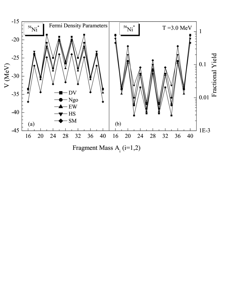
Figure 3: (a) The fragmentation potential $V(\eta)$ and (b) calculated fission mass distribution yield with different density parameters at $T$ = 3.0 MeV.

Fig. 3(a) and (b) shows the fragmentation potential $V(\eta)$ and fractional yield at $R=R_{min}$ with $V(R_{min})=\overline{V}_{min}$. The fractional yields are calculated within PCM at $T$ = 3.0 MeV using various Fermi density parameters for ⁵⁶Ni^∗. From figure, we observe that different parameters have minimal role in the fractional mass distribution yield. The fine structure is not at all disturbed for different sets of Fermi density parameters.

We have also calculated the half-life times (or decay constants) of ⁵⁶Ni^∗ within PCM and UFM for clusters $\geq^{16}$O. For ¹⁶O, the cluster decay constant varies by an order of magnitude ten. The variation is much more with SM parameters. In the case of UFM, variation is almost constant.

In Fig. 4, we display the cluster decay half-lives $\log T_{1/2}$ for various Fermi density parameters using PCM. There is smooth variation in half-life times with all the density parameters except for SM parameter. The trends in the variation of cluster half-life times (or decay constants) are similar in both PCM and UFM, but in case of UFM decay constants are more by an order of ten. In SM the decay constants are larger by an order of 14.

In order to quantify the results, we have also calculated the percentage variation in $\log T_{1/2}$ as:

$$\left[\log T_{1/2}\right]\%=\frac{(\log T_{1/2})^{i}-(\log T_{1/2})^{DV}}{(\log T_{1/2})^{DV}}\times 100,$$ (39)

where $i$ stands for the half-life times calculated using different Fermi density parameters. The variation in the cluster decay half-lives is studied with respect to DV parameters. In Fig. 5(a) and (b), we display the percentage variation in the half-life times within both the PCM and UFM models as a function of cluster mass $A_{2}$ using Eq. (39). For the PCM these variation lies within $\pm$5% excluding SM parameters, whereas including SM parameters it lies within $\pm$13%. In the case of UFM half-lives lies within $\pm$1.5% for all density parameters except of SM. For SM parameters variations lie within $\pm$9%.

Finally, it would be of interest to see how different forms of nuclear radii as discussed earlier would affect the cluter decay half-lives.

In Fig. 6, we display the characteristic scattering potential for the cluster decay of ⁵⁶Ni^∗ into ²⁸Si + ²⁸Si channel for R_Bass and R_Royer forms of nuclear radius. In the exit channel for the compound nucleus to decay, the compound nucleus excitation energy $E_{CN}^{\ast}$ goes in compensating the negative $Q_{out}$, the total excitation energy $TXE$ and total kinetic energy $TKE$ of the two outgoing fragments as the effective Q-value. We plot the penetration path for PCM using Skyrme force SIII (without surface correction factor, $\lambda=0$) with nuclear radius R_Bass. Here again, we begin the penetration path at $R_{a}=R_{min}$ with potential at this $R_{a}$-value as $V(R_{a}=R_{min})=\overline{V}_{min}$ and ends at $R=R_{b}$, corresponding to $V(R=R_{b})=Q_{eff}$ for PCM. The $Q_{eff}$ are same as discussed earlier.

Fig. 7(a) and (b) show the fragmentation potentials $V(\eta)$ and fractional yields at $R=R_{min}$ with $V(R_{min})=\overline{V}_{min}$. The fractional yields are calculated within PCM at $T$ = 3.0 MeV for ⁵⁶Ni^∗ using various forms of nuclear radii. From figure, we observe that different radii gives approximately similar behavior, however small changes in the fractional mass distribution yields are observed. The fine structure is not at all disturbed for different radius values.

We have also calculated the half-life times (or decay constants) of ⁵⁶Ni^∗ within PCM for clusters $\geq^{16}$O. The cluster decay constant for nuclear radius due to Bass varies by an order of magnitude $10^{2}$, where as order of magnitude is same for other radii. In Fig. 8, we display the cluster decay half-lives $\log T_{1/2}$ for various nuclear radii taken by different authors as explained earlier using PCM. One can observe small variations in half-life times.

In order to quantify the results, we have also calculated the percentage variation in $\log T_{1/2}$ as:

$$\left[\log T_{1/2}\right]\%=\frac{(\log T_{1/2})^{i}-(\log T_{1/2})^{R_{Royer}}}{(\log T_{1/2})^{R_{Royer}}}\times 100,$$ (40)

where $i$ stands for the half-life times calculated using different forms of nuclear radii. The variation in the cluster decay half-lives is studied with respect to radius formula given by Royer R_Royer. In Fig. 9, we display the percentage variation in the half-life times for PCM as a function of cluster mass $A_{2}$ using Eq. (40). These variation lies within $\pm$7% excluding Bass radius where it lies within $\pm$10%.

4 Summary

We here reported the role of various model ingredients as well as radii in the cluster decay constant calculations. Our studies revealed that the effect of different density and nuclear radius parameters on the cluster decay half-life times is about $10\%$. Our study justify the use of current set of parameters for radius as the effect of different prescriptions is very small.

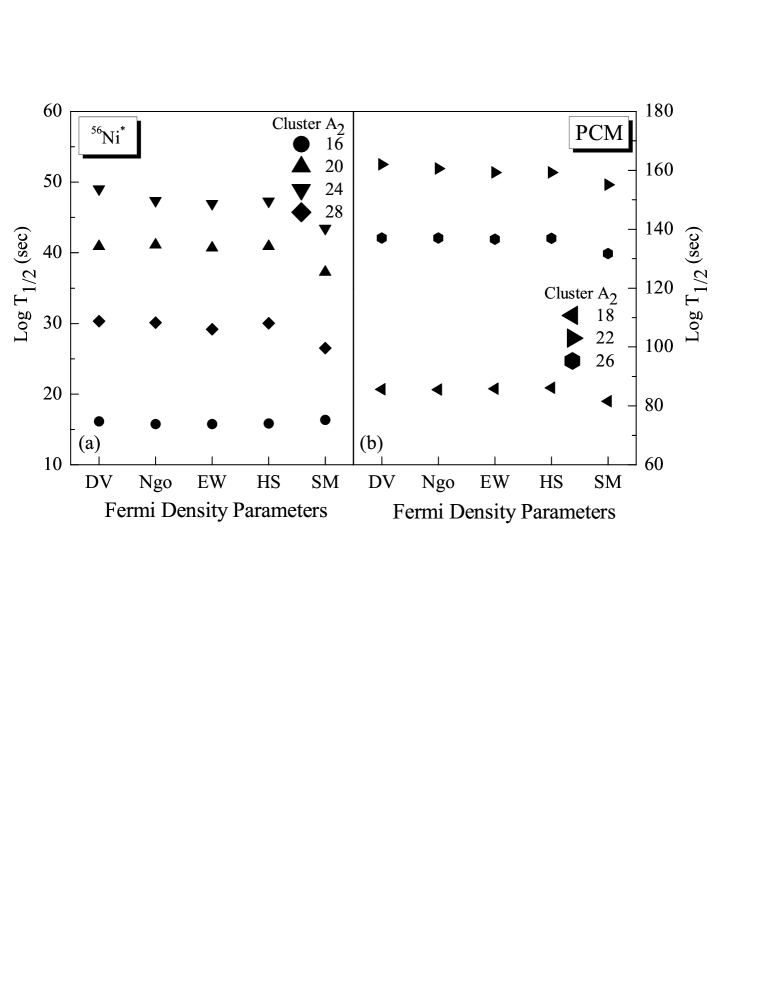
Figure 4: The variation of $\log T_{1/2}$ (sec) using different density parameters for PCM.

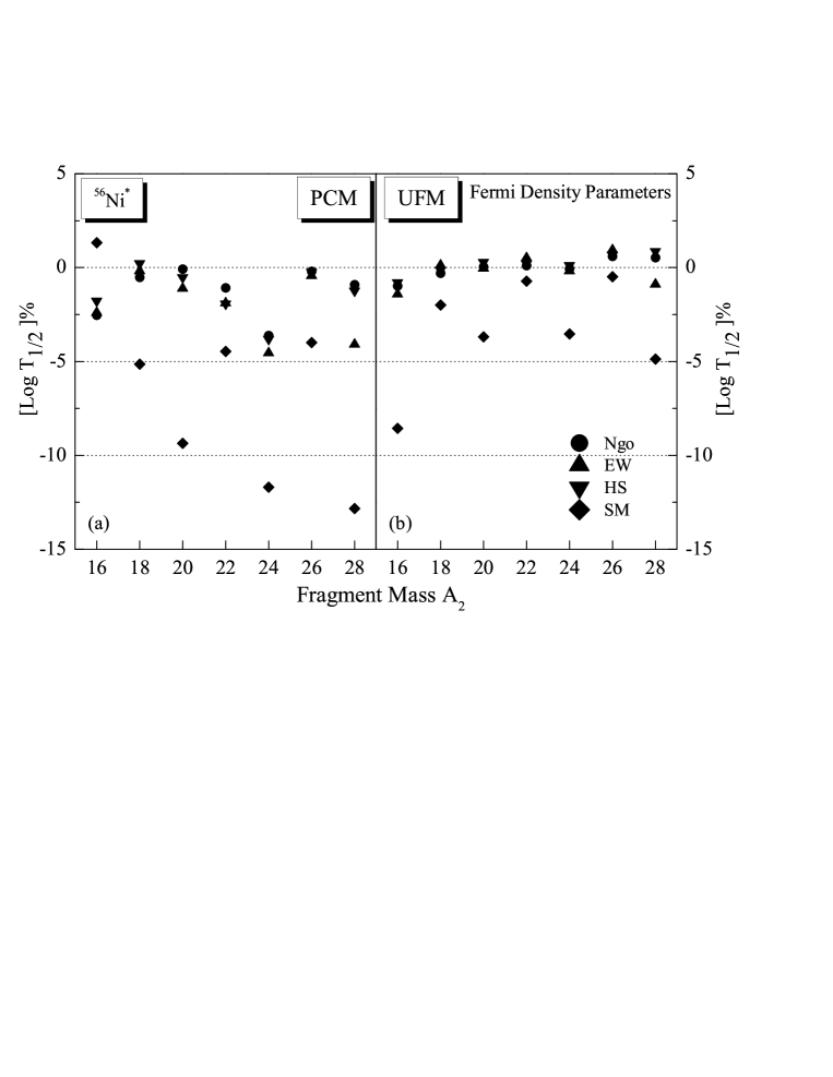
Figure 5: Percentage variation of $\log T_{1/2}$ for different different Fermi density parameters w.r.t. DV parameters.

Figure 6: Same as fig. 2, but for different radii. The decay path displayed only for PCM.

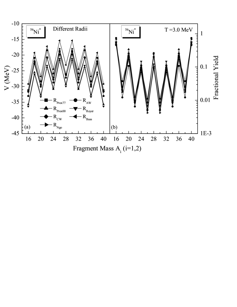
Figure 7: Same as fig. 3, but for different radii.

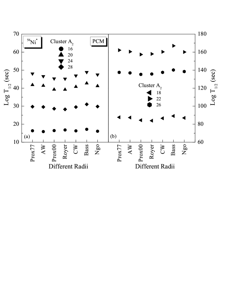
Figure 8: Same as fig. 4, but for different radii.

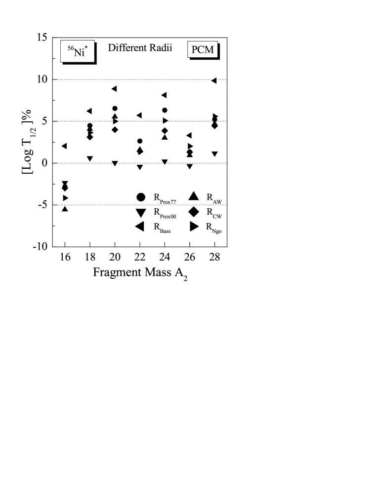
Figure 9: Percentage variation of $\log T_{1/2}$ for different forms of radii with PCM only.

References

- [1] I. Angeli, et al., J. Phys. G: Nucl. Part. Phys. 6, 303 (1980).
- [2] E. Wesolowski, et al., J. Phys. G: Nucl. Part. Phys. 10, 321 (1984).
- [3] J. Friedrich, N. Vögler Nucl. Phys. A 373, 192 (1982).
- [4] S. Kumar et al., Phys. Rev. C 58, 3494 (1998); ibid. C 58, 1618 (1998); J. Singh et al., Phys. Rev. C 62, 044617 (2000); E. Lehmann et al., Phys. Rev. C 51, 2113 (1995); R.K. Puri et al., Nucl. Phys. A 575, 733 (1994); D.T. Khoa et al., Nucl. Phys. A 548, 102 (1992); S.W. Huang et al., Phys. Lett. B 298, 41 (1993); G. Batko et al., J. Phys. G: Nucl. Part. Phys. 20, 461 (1994); S.W. Huang et al., Prog. Part. Nucl. Phys. 30, 105 (1993); E. Lehmann et al., Prog. Part. Nucl. Phys. 30, 219 (1993).
- [5] R.K. Puri et al., Phys. Rev. C 54, R28 (1996); ibid. J. Comput. Phys. 162, 245 (2000); A. Sood et al., Phys. Rev. C 70, 034611 (2004); S. Kumar et al., Phys. Rev. C 81, 014601 (2010); ibid. C 78, 064602 (2009); P.B. Gossiaux et al., Nucl. Phys. A 619, 379 (1997); C. Fuchs et al., J. Phys. G: Nucl. Part. Phys. 22, 131 (1996).
- [6] C. Ngô et al., Nucl. Phys. A 252, 237 (1975); H. Ngô, C. Ngô, Nucl. Phys. A 348, 140 (1980).
- [7] R.K. Puri, N.K. Dhiman, Eur. Phys. J. A 23, 429 (2005); R. Arora et al., ibid. 8, 103 (2000); R.K. Puri et al., ibid. 3, 277 (1998); R.K. Puri et al., Phys. Rev. C 51, 1568 (1995); ibid. 45, 1837 (1992); ibid. J. Phys. G: Nucl. Part. Phys. 18, 903 (1992); R.K. Puri, R.K. Gupta, Int. J. Mod. Phys. E 1, 269 (1992).
- [8] S.A. Moszkwski, Nucl. Phys. A 309, 273 (1978).
- [9] E. Wesolowski, J. Phys. G: Nucl. Part. Phys. 11, 909 (1985).
- [10] H. Schechter et al., Nucl. Phys. A 315, 470 (1979).
- [11] L.R.B. Elton, Nuclear sizes, Oxford University Press, London (1961); H. de Vries, C.W. de Jager, C.de Vries, At. Data Nucl. Data Tables 36, 495 (1987).
- [12] R.K. Gupta et al., J. Phys. G: Nucl. Part. Phys. 18, 1533 (1992).
- [13] R. Arora, Ph. D. Thesis, Panjab University, Chandigarh (2003).
- [14] J.M.B. Shorto et al., Phys. Rev. C 81, 044601 (2010); I. Dutt, R.K. Puri ibid. 81, 047601 (2010); ibid. 81, 044615 (2010); ibid. 81, 064609 (2010); ibid. 81, 064608 (2010).
- [15] C. Xu, B.A. Li Phys. Rev. C 81, 044603 (2010); S. Kumar ibid. 78, 064602 (2008); ibid. 81, 014611 (2010); ibid. 81, 014601 (2010); Y.K. Vermani et al., J. Phys. G: Nucl. Part. Phys. 36, 105103 (2010); ibid. 37, 015105 (2010); ibid. Europhys. lett. 85, 62001 (2009); ibid. Phys. Rev. C 79, 064613 (2009); A. Sood et al., ibid. 79, 064618 (2009); S. Gautam et al., J. Phys. G: Nucl. Part. Phys. 37, 085102 (2010); ibid. Phys. Rev. C 83, 014603 (2011); ibid. Phys. Rev. C 83, 034606 (2011); R. Chugh et al., Phys. Rev. C 82, 014603 (2010); S. Goyal et al., Nucl. Phys. A 847, 164 (2011); ibid. Phys. Rev. C 83, 047601 (2011); V. Kaur et al., Phys. Lett. B 697, 512 (2011); ibid. Nucl. Phys. A 861, 36 (2011).
- [16] S.K. Patra et al., Phys. Rev. C 80, 034612 (2009); S.K. Arun et al., ibid. 80, 034317 (2009); ibid. 79, 064616 (2009); R. Kumar et al., ibid. 79, 034602 (2009).
- [17] K.P. Santhosh et al., J. Phys. G: Nucl. Part. Phys. 36, 115101 (2009); ibid. 36, 015107 (2009); Pramana J. Phys. 59, 599 (2002).
- [18] R.K. Gupta, 5th International Conference on Nuclear Reaction Mechanisms, Varenna, Italy, p. 416 (1988).
- [19] S.S. Malik, R.K. Gupta, Phys. Rev. C 39, 1992 (1989); ibid. C 50, 2973 (1994); S.S. Malik et al., Pramana J. Phys. 32, 419 (1989); R.K. Gupta et al., Phys. Rev. C 47, 561 (1993).
- [20] S. Kumar, R.K. Gupta, Phys. Rev. C 55, 218 (1997); ibid. C 49, 1922 (1994).
- [21] D.N. Poenaru, W. Greiner, R. Gherghescu, Phys. Rev. C 47, 2030 (1993); H.F. Zhang et al., ibid. 80, 037307 (2009).
- [22] B. Buck, A.C. Merchant, S.M. Perez, Nucl. Phys. A 512, 483 (1990); B. Buck, A.C. Merchant, J. Phys. G: Nucl. Part. Phys. 16, L85 (1990).
- [23] A. Sandulescu et al., Int. J. Mod. Phys. E 1, 379 (1992); R.K. Gupta, et al., J. Phys. G: Nucl. Part. Phys. 19, 2063 (1993); Phys. Rev. C 56, 3242 (1997).
- [24] D. Vautherin, D.M. Brink, Phys. Rev. C 5, 626 (1972).
- [25] P. Chattopadhyay, R.K. Gupta, Phys. Rev. C 30, 1191 (1984), and earlier references therein.
- [26] C.F. von Weizsäcker, Z. Phys. 96, 431 (1935).
- [27] D.M. Brink, F. Stancu, Nucl. Phys. A 243, 175 (1975); F. Stancu, D.M. Brink, ibid, A 270, 236 (1976).
- [28] R.K. Puri, P. Chattopadhyay, R.K. Gupta, Phys. Rev. C 43, 315 (1991).
- [29] J. Blocki et al., Ann. Phys. 105, 427 (1977).
- [30] A. Winther, Nucl. Phys. A 594, 203 (1995).
- [31] W.D. Myers, W.J. Światecki, Phys. Rev. C 62, 044610 (2000).
- [32] G. Royer, R. Rousseau, Eur. Phys. J. A 42, 541 (2009).
- [33] R. Bass, Phys. Lett. B 47, 139 (1973).
- [34] P.R. Christensen, A. Winther, Phys. Lett. B 65, 19 (1976).
- [35] R.K. Gupta et al., J. Phys. G: Nucl. Part. Phys. 26, L23 (2000).
- [36] R.K. Gupta, W. Scheid, W. Greiner, Phys. Rev. Lett. 35, 353 (1975).
- [37] D.R. Saroha, N. Malhotra, R.K. Gupta, J. Phys. G: Nucl. Part. Phys. 11, L27 (1985).
- [38] J. Maruhn, W. Greiner, Phys. Rev. Lett. 32, 548 (1974).
- [39] A. Sandulescu, D.N. Poenaru, W. Greiner, Sovt. J. Part. Nucl. 11, 528 (1980).
- [40] H.J. Rose, G.A. Jones, Nature (London) 307, 245 (1984).
- [41] R.K. Gupta, W. Greiner, Int. J. Mod. Phys. E 3, 335 (1994).
- [42] P. Möller et al., At. Data Nucl. Data Tables 59, 185 (1995).
- [43] H. Kröger, W. Scheid, J. Phys. G: Nucl. Part. Phys. 6, L85 (1980).
- [44] N.K. Dhiman, I. Dutt, Pramana J. Phys. 76, 441 (2011).
- [45] M.K. Sharma, R.K. Gupta, W. Scheid, J. Phys. G: Nucl. Part. Phys. 26, L45 (2000).