Vacuum Stability of the wrong sign $(-\phi^{6})$ Scalar Field Theory

Abstract

We apply the effective potential method to study the vacuum stability of the bounded from above $(-\phi^{6})$ (unstable) quantum field potential. The stability ($\partial E/\partial b=0)$ and the mass renormalization ($\partial^{2}E/\partial b^{2}=M^{2})$ conditions force the effective potential of this theory to be bounded from below (stable). Since bounded from below potentials are always associated with localized wave functions, the algorithm we use replaces the boundary condition applied to the wave functions in the complex contour method by two stability conditions on the effective potential obtained. To test the validity of our calculations, we show that our variational predictions can reproduce exactly the results in the literature for the $\mathcal{PT}$-symmetric $\phi^{4}$ theory. We then extend the applications of the algorithm to the unstudied stability problem of the bounded from above $(-\phi^{6})$ scalar field theory where classical analysis prohibits the existence of a stable spectrum. Concerning this, we calculated the effective potential up to first order in the couplings in $d$ space-time dimensions. We find that a Hermitian effective theory is instable while a non-Hermitian but $\mathcal{PT}$-symmetric effective theory characterized by a pure imaginary vacuum condensate is stable (bounded from below) which is against the classical predictions of the instability of the theory. We assert that the work presented here represents the first calculations that advocates the stability of the $(-\phi^{6})$ scalar potential.

I Introduction

The very active research area of the non-Hermitian theories with real spectra bender ; aboebt ; ghost ; aboeff ; bendvs ; spect ; nonr ; spect1 ; ghost1 ; ghost2 may offer solutions to current existing problems in our understanding of nature. Among the very large number of non-Hermitian theories investigated, theories with bounded from above potentials deserve more interest than what offered in the literature. In their quantum field versions, such theories possess the very important asymptotic freedom property aboebt ; Symanzik ; bendf ; Frieder . To shed light on the importance of this property, one has to mention that in the past, to have such interesting property, physicists had to resort to a somehow complicated model which merges group theory to field theory with the number of colors to be equal to or greater than three (quantum chromodynamics). Now and after the discovery of possible physical acceptability of some of the non-Hermitian theories, one can get the important asymptotic freedom property from just colorless, one component and scalar field theories.

Apart from the above mentioned benefits that can be obtained from the employment of the non-Hermitian theories in our modeling of natural events, a big problem was thought to exist in dealing with such theories. In fact, for physical amplitude calculations in the non-Hermitian theories, the metric operator formulations are indispensable. However, the suggested regimes for metric operator calculations in the literature turns the theory divergent even at the quantum mechanical level of study bendvs . For Higher dimensions, the degree of divergences will be even higher and the calculation of the metric operator becomes complicated and even hard to get in a closed form for some perturbative calculations bendmet . However, Jones and Rivers showed that in case of metric operator of gauge form, one can get physical amplitudes from path integrals within the non-Hermitian theory jonesqds . Moreover, it has been shown that the effective field approach does know about the metric jonesgr1 ; jonesgr2 and since effective field approach can be easily extended to the important quantum field case aboeff ; aboebt , one may not worry about the metric any more.

The complex contour method followed in the literature, apart from its success, is hard to follow specially for the study of non-Hermitian quantum field theories. In this approach, one finds a contour in the complex $\ x$-plane ($x$ is equivalent to the field variable in our work) on which the wave functions are localized in the sense that a wave function vanishes as $\left|x\right|\rightarrow 0$. To avoid the problem of finding a contour of such characteristics, one can think in taking the imaginary part of $x$ as a variational parameter that can be adapted in such away that secures the localization of wave functions. However, the process is similar to a field shift which is a well known method in the literature through which one can obtain the corresponding effective potential. The challenge now is to map the boundary condition on wave functions on a complex contour to a condition on the effective potential. In fact, our experience in solving quantum mechanical problems tells us that bounded from below potentials results in localized wave function. Accordingly, one can replace localized wave function boundary condition in the complex contour method by constraining the parameters in the effective potential in such away that turns it bounded from below (stable).

Although one can follow path integral to calculate the effective potential, in this work we follow the canonical quantization method efbook ; Peskin ; Coleman ; normal2 ; Canon1 ; changcac ; mag to calculate the effective potential. In fact, in the context of non-Hermitian theories, it would be more suitable to follow the Canonical quantization method as the Hamiltonian operator can reflect the non-Hermiticity of a theory more clearer than dealing with classical functions in the path integral formalism. The organization of the paper is as follows. In section II, we introduce the formulation of the effective potential within the canonical quantization method. In section III, we study the quantum mechanical case ($0+1$ dimensions). In section IV, we study the the wrong sign $(-\phi^{6})$ scalar field theory in $1+1$ and $2+1$ space-time dimensions. Also, in section V, we test our results by presenting comparisons with those available in the literature while conclusion follows in section VI.

II The Calculation of the effective potential

To start, consider the quantum field Hamiltonian density of the form;

$$H=\frac{1}{2}\left(\triangledown\phi\right)^{2}+\frac{1}{2}\pi^{2}+\frac{1}{2}m^{2}\phi^{2}+g\phi^{4}+h\phi^{6},$$ (1)

where $m$ is the mass of the field $\phi$, $\pi$ is the conjugated momentum field while $g$ and $h$ are coupling constants. The mean field approach is lunched by the application of the canonical transformation $\phi=\psi+B$ and $\pi=\Pi$. Here, $B$ is a constant called the vacuum condensate and $\Pi=\overset{\cdot}{\psi}$. The philosophy behind the field shift is to account in variational manner for the imaginary part of the complex contour method followed in the literature jones ; bender . This field shift will lead to an effective potential on which one may apply constraints that is equivalent to the boundary condition on a complex contour. In the literature, we get used to have localized wave functions associated with bounded from below potentials in quantum mechanical problems. Accordingly, one can constrain the effective potential to be bounded from below and don’t exclude values of the parameters that turn the theory non-Hermitian. Equivalently, we map the condition $\chi\left(x\right)\rightarrow 0$ as $\left|x\right|\rightarrow\infty$ ( $\chi\left(x\right)$ is the wave function) in the complex contour algorithm to the constraint on the effective potential that enforces it to be bounded from below. In this way we obtain a more practical algorithm to do calculations even in complicated non-Hermitian field theories for which one may fail to follow the complex contour algorithm.

Plugging the above transformations into the Hamiltonian model in Eq.(1) to get an equivalent effective form as;

$$H =\frac{1}{2}\left(\triangledown\psi\right)^{2}+\frac{1}{2}\Pi^{2}+\frac{1}{2}M^{2}\psi^{2}+\left(15hB^{4}+6gB^{2}+\frac{1}{2}m^{2}-\frac{1}{2}M^{2}\right)\psi^{2}$$

$$+\left(20hB^{3}+4gB\right)\allowbreak\psi^{3}+\left(15hB^{2}+g\right)\psi^{4}+6Bh\psi^{5}+h\psi^{6}$$ (2)

$$+\left(6hB^{5}+4gB^{3}+Bm^{2}\right)\allowbreak\psi+\left(hB^{6}+gB^{4}+\frac{1}{2}B^{2}m^{2}\right).$$

We have chosen to work with the mass parameter $M$ ( which collects all the coefficients of $\psi^{2}$) of the field $\psi$  and consider all terms except the kinetic term $(\frac{1}{2}\left(\triangledown\psi\right)^{2}+\frac{1}{2}\Pi^{2}+\frac{1}{2}M^{2}\psi^{2})$ to constitute an interaction Hamiltonian. The vacuum expectation value of the Hamiltonian operator $\langle\Omega\left|H\right|\Omega\rangle$ is known as the effective potential or vacuum energy, where $|\Omega\rangle$ represents the vacuum state of the interacting theory. In the canonical quantization regime ( the first part of Ref. Peskin ), one can calculate the expectation value of an operator in an interactive theory in terms of the free vacuum state $|0\rangle$ via the employment of the time evolution operator ( Eq. (4.31) in Ref. Peskin ). At the tree level, the vacuum energy is given by;

$$\langle\Omega\left|H\right|\Omega\rangle=E=hB^{6}+gB^{4}+\frac{1}{2}B^{2}m^{2}.$$

In this form one realizes that;

$$\frac{\partial E}{\partial B}=6hB^{5}+4gB^{3}+Bm^{2},$$

which is exactly the coefficient of the linear term in the field $\psi$ in Eq.(2). This term has to be dropped out if  one seeks the stability of the theory and this term will disappear order by order Peskin . Another realization is that $\frac{\partial^{2}E}{\partial B^{2}}$ is known to be equal to $i\left(\frac{i}{p^{2}-M^{2}}\right)^{-1}$, with $p$ as the external momentum swanson . Since $B$ is position independent, then the external momentum is certainly zero. So one can employ the constraints;

$$\frac{\partial E}{\partial B}=0\text{ and }\frac{\partial^{2}E}{\partial B^{2}}=M^{2},$$ (3)

on the parameters $B$ and $M$. If $M^{2}$ is to be chosen positive, this means that the effective potential $E$ is bounded from below and thus stable. In our work we will use the conditions in Eq. (3) to mimic the localized wave function boundary condition in the complex contour method in Ref.bender .

For the first order correction ( in the couplings) to the effective potential, we consider the Feynman diagrams contributing to this order shown in Fig.1.  Note that, one can split the vacuum expectation value of the Hamiltonian as $\langle\Omega\left|H\right|\Omega\rangle=\langle\Omega\left|H_{0}\right|\Omega\rangle+\langle\Omega\left|H_{I}\right|\Omega\rangle$, where the Hamiltonian operator $H$ has been decomposed into the free Hamiltonian $H_{0}$ plus the interaction Hamiltonian $H_{I}$. In fact, $H_{0}$ is diagonal with respect to the free vacuum and thus can easily obtained to be;

$$\langle\Omega\left|H_{0}\right|\Omega\rangle=\frac{1}{2\left(4\pi\right)^{\frac{d-1}{2}}}\left(\frac{\Gamma\left(-\frac{1}{2}-\frac{d-1}{2}\right)}{\Gamma\left(-\frac{1}{2}\right)}\left(\frac{1}{M^{2}}\right)^{-\frac{1}{2}-\frac{d-1}{2}}\right),$$

and the the expectation value of the interaction Hamiltonian $\langle\Omega\left|H_{I}\right|\Omega\rangle$  can be obtained perturbatively. Note that the diagrams generated by the amplitude $\langle\Omega\left|H_{I}\right|\Omega\rangle$ do not have external legs (zero momentum) because the Hamiltonian itself is an integration over the position space of the Hamiltonian density $H$. In other words, the diagrams contributing to the amplitude $\langle\Omega\left|H_{I}\right|\Omega\rangle$ are those generated by fully contracted internal lines.

Up to first order in the couplings, the fully contracted diagrams of the theory under investigation are given in Fig. 1. Accordingly, one can get the result of $\langle\Omega\left|H_{I}\right|\Omega\rangle$ for $d$ space-time dimensions as;

$$E =\frac{1}{2\left(4\pi\right)^{\frac{d-1}{2}}}\left(\frac{\Gamma\left(-\frac{1}{2}-\frac{d-1}{2}\right)}{\Gamma\left(-\frac{1}{2}\right)}\left(\frac{1}{M^{2}}\right)^{-\frac{1}{2}-\frac{d-1}{2}}\right)+\frac{1}{2}B^{2}m^{2}+gB^{4}+hB^{6}+\left(\frac{-i6!h}{-3!\times 8i}\right)\left(\Delta\right)^{3}$$

$$+\left(\frac{-i4!\left(15hB^{2}+g\right)}{-i8}\right)\left(\Delta\right)^{2}+\left(\frac{-i2\left(15hB^{4}+6gB^{2}+\frac{1}{2}m^{2}-\frac{1}{2}M^{2}\right)}{-i2}\right)\left(\Delta\right),$$ (4)

where

$$\Delta=\frac{1}{\left(4\pi\right)^{\frac{d}{2}}}\frac{\Gamma\left(1-\frac{d}{2}\right)}{\Gamma\left(1\right)}\left(\frac{1}{M^{2}}\right)^{1-\frac{d}{2}},$$

and $\Gamma$ is the gamma function.This form of the vacuum energy is finite in $0+1$ space-time dimensions but for higher dimensions divergences are existing and need certain procedures to get red out of them.

III the effective potential of the $\mathcal{PT}$-symmetric $(-\phi^{6})_{0+1}$ theory

For $d=1$ (quantum mechanics), $E$ can be simplified as;

$$E=\frac{1}{2}M+\frac{1}{2}B^{2}m^{2}+gB^{4}+hB^{6}+\frac{3}{4}\frac{\left(15hB^{2}+g\right)}{M^{2}}+\frac{15}{8}\frac{h}{M^{3}}+\frac{1}{4M}\left(30hB^{4}+12gB^{2}-M^{2}+m^{2}\right).$$ (5)

For this effective potential to be stable, one has to constrain the parameters introduced in the calculations such that;

$$\frac{\partial E}{\partial B}=0.$$

Let us first study the case of $g=0$ and $m=0$, where we get the result;

$$\frac{3}{2}\frac{B}{M^{2}}h\left(4B^{4}M^{2}+20B^{2}M+15\right)=0.$$ (6)

This equation has three different solutions of the form;

$$B =0,$$

$$B^{2} =-\frac{1}{2M}\left(\sqrt{10}+5\right),\text{ }$$ (7)

$$B^{2} =\frac{1}{2M}\left(\sqrt{10}-5\right).$$

The $B=0$ solution is acceptable only for the bounded from below theory (positive $h)$. In this case the theory is Hermitian and the vacuum is stable as well. For the solutions $B^{2}=-\frac{1}{2M}\left(\sqrt{10}+5\right)$ and $B^{2}=\frac{1}{2M}\left(\sqrt{10}-5\right)$, $M$ is positive and thus $B$ is imaginary. Accordingly, the Hamiltonian form in Eq.(2) is non-Hermitian but $\mathcal{PT-}$symmetric as well and one then can claim that the spectrum of the theory is real and stable for both broken symmetry solutions in Eq.(7) either $h$ positive or negative. In fact, the story here is different and it is only the solution $B^{2}=-\frac{1}{2M}\left(\sqrt{10}+5\right)$ that is stable for the bounded from below potential $\left(+h\right)$ while the solution $B^{2}=\frac{1}{2M}\left(\sqrt{10}-5\right)$ represents an unstable vacuum. In fact, for the solution $B^{2}=-\frac{1}{2M}\left(\sqrt{10}+5\right)$ , the effective potential has the form;

$$E=-\frac{1}{B^{2}\left(136\sqrt{10}+440\right)}\left(\left(64h+32\sqrt{10}h\right)B^{8}+140\sqrt{10}+445\right)\allowbreak,$$

which shows that $E$ with $B$ real is $-E$ with $B$ imaginary. In fact, real $B$ means that $M$ is negative which means the existence of ghost states (negative kinetic energy).

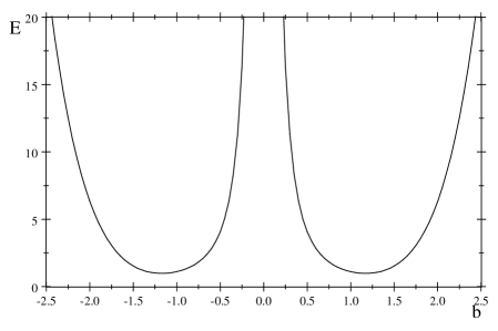
Figure 2: The ground state energy as a function of the one-point function $B\equiv\left\langle 0|\phi|0\right\rangle\equiv ib$ measured in units of $i$ for $h=0.5$ for the solution $B^{2}=-\frac{1}{2M}\left(\sqrt{10}+5\right)$ of the $\mathcal{PT}$-symmetric $\phi^{6}$ potential.

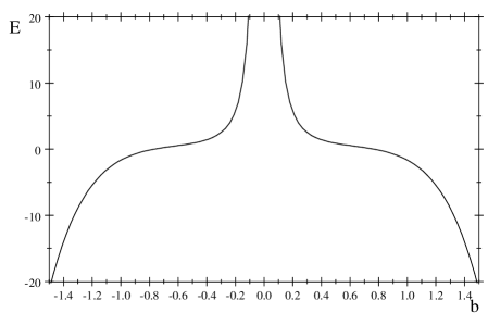
Figure 3: The ground state energy as a function of the one-point function measured in units of $i$ for $h=0.5$ for the the solution $B^{2}=\frac{1}{2M}\left(\sqrt{10}-5\right)$ of the $\mathcal{PT}$-symmetric $\phi^{6}$ potential.

In this article we shall stick to the usual understanding of particles as they have positive masses and stability exists from minimizing actions. Consequently, $B$ is chosen imaginary and to investigate the stability of the theory we plot the diagram in Figs.2 where one can realize that the effective potential (vacuum energy ) is bounded from below for $h=+\frac{1}{2}$ for the solution $B^{2}=-\frac{1}{2M}\left(\sqrt{10}+5\right)$ . On the other hand, the solution $B^{2}=\frac{1}{2M}\left(\sqrt{10}-5\right)$ results in an instable vacuum since the associated effective potential is unbounded either from above or from below (Fig. 3). Again with the solution $B^{2}=\frac{1}{2M}\left(\sqrt{10}-5\right)$, the effective potential has the form;

$$E=\frac{1}{B^{2}\left(136\sqrt{10}-440\right)}\left(\left(64h-32\sqrt{10}h\right)B^{8}-140\sqrt{10}+445\right)\allowbreak,$$

which for $B$ real has exactly an opposite sign to the imaginary $B$ result.

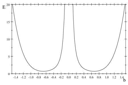
Figure 4: The ground state energy as a function of the one-point function measured in units of $i$ for $h=-0.5$ for the the solution $B^{2}=\frac{1}{2M}\left(\sqrt{10}-5\right)$ of the $\mathcal{PT}$-symmetric $\phi^{6}$ potential.

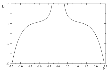
Figure 5: The ground state energy as a function of the one-point function measured in units of $i$ for $h=-0.5$ for the solution $B^{2}=-\frac{1}{2M}\left(\sqrt{10}+5\right)$ of the $\mathcal{PT}$-symmetric $\phi^{6}$ potential.

For an unstable classical potential (negative $h$ coupling), on the other hand, the solution $B^{2}=\frac{1}{2M}\left(\sqrt{10}-5\right)$ results in a stable effective potential as shown in Fig.4 while the solution $B^{2}=-\frac{1}{2M}\left(\sqrt{10}+5\right)$ is unstable (Fig.5). These results are in fact very interesting since they show that stability (like tunneling) can not always be argued in view of classical analysis. A classically stable potential may or may not lead to a stable quantized system. The reverse is also correct, a classically instable potential can have stable as well as instable spectra.

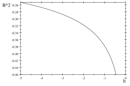
Figure 6: The one-point function squared versus the coupling $h$ for the massless $\mathcal{PT}$-symmetric $(-\phi^{6})$ potential in $0+1$ space-time dimensions.

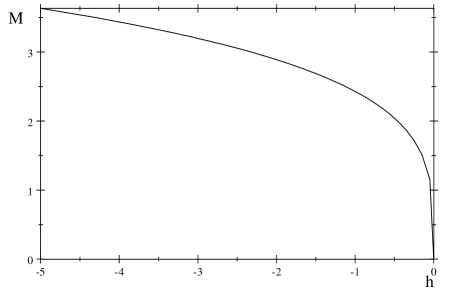
Figure 7: The effective mass of the field $\psi$ versus the coupling $h$ for the massless $\mathcal{PT}$-symmetric $(-\phi^{6})$ potential in $0+1$ space-time dimensions.

For the bounded from above potential (negative $h)$ the $B=0$ solution is unstable. Accordingly, only the broken symmetry solution characterized by the parameters $B^{2}=\frac{1}{2M}\left(\sqrt{10}-5\right)$ and $M=\sqrt[4]{-30\left(\sqrt{10}-2\right)h}$ is the only acceptable solution. For this case, the behavior of the vacuum condensate as a function of the coupling $h$ is shown in Fig.6 while the behavior of the effective mass $M$ is presented in Fig.7.

The results above show that the algorithm we follow is reliable in studying non-Hermitian theories. A big advantage of this algorithm is that it can be extended easily to theories which have never been studied like the bounded from above theories with many couplings.

In $d$ space-time dimensions, for the general case of massive theory as well as for $g\neq 0$, we get the results;

$$M =\frac{1}{\left(15^{\frac{1}{-2+d}}\right)}2^{\frac{d}{-2+d}}\pi^{\frac{d}{2\left(-2+d\right)}}\frac{\left(-2g-10B^{2}h+\sqrt{4g^{2}+40B^{4}h^{2}-10hm^{2}}\right)^{\frac{1}{-2+d}}}{\left(h^{\frac{1}{-2+d}}\right)\left(\left(-\Gamma\left(-\frac{1}{2}d\right)d\right)^{\frac{1}{-2+d}}\right)}\allowbreak,$$

$$M =\frac{1}{\left(15^{\frac{1}{-2+d}}\right)}2^{\frac{1}{-2+d}d}\pi^{\frac{1}{2\left(-2+d\right)}d}\frac{\left(-2g-10B^{2}h-\sqrt{4g^{2}+40B^{4}h^{2}-10hm^{2}}\right)^{\frac{1}{-2+d}}}{\left(h^{\frac{1}{-2+d}}\right)\left(\left(-\Gamma\left(-\frac{1}{2}d\right)d\right)^{\frac{1}{-2+d}}\right)}\allowbreak$$ (8)

For the $0+1$ case, we get;

$$\frac{E}{m}=e=-Hb^{6}+\left(\frac{15}{2t}H+G\right)b^{4}-\left(\frac{45}{4t^{2}}H+\frac{3}{t}G+\frac{1}{2}\right)b^{2}+\frac{1}{4}t+\allowbreak\frac{3}{4t^{2}}G+\frac{15}{8t^{3}}H+\frac{1}{4t},$$ (9)

where we introduced the dimensionless parameters $b$, $H$, $G$ and $t$ as $B=m^{\frac{d-2}{2}}\frac{b}{i}$, $h=Hm^{-2d+6}$, $g=Gm^{-d+4}$ and $M=tm$. In this case we can obtain the dimensionless mass $t=\frac{M}{m}$ of the form;

$$t=\frac{-15H}{2G-10b^{2}H+\sqrt{4G^{2}+40b^{4}H^{2}-10H}},\allowbreak$$

$$t=\frac{-15H}{2G-10b^{2}H-\sqrt{4G^{2}+40b^{4}H^{2}-10H}}\allowbreak.$$

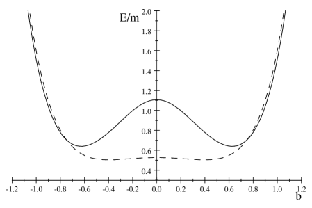
Figure 8: The $0+1$ space-time dimensions effective potential as a function of the one-point function measured in units of $i$ for $H=-\frac{1}{4}\mathtt{,}G=+\frac{1}{2}$ (dashed) and $H=-\frac{1}{4}\mathtt{,}G=-\frac{1}{2}$ (solid) with the stable solution $t=\frac{-15H}{2G-10b^{2}H+\sqrt{4G^{2}+40b^{4}H^{2}-10H}}$ of the $\mathcal{PT}$-symmetric $\phi^{6}$ potential.

As we can see from Fig.8, the effective potential is bounded from below (stable) for negative $H$ and for $\pm G$ but only for the solution;

$$t=\frac{-15H}{2G-10b^{2}H+\sqrt{4G^{2}+40b^{4}H^{2}-10H}}.$$

In the above calculations, although we used dimensional regularization to calculate the Feynman diagrams, $E$ is finite even in using direct integral calculations. In higher dimensions, however, $E$ is divergent even in using the dimensional regularization and thus one has to follow one of other known procedures to kill the divergences.

IV The effective potential in higher space-time dimensions

For higher space-time dimensions, the dimensional regularization used to calculate the Feynman diagrams leaded to the above results may not be able to get rid of the existing divergences. For instance, in $1+1$ space-time dimensions, the gamma function, $\Gamma\left(1-\frac{1}{2}d\right)$, is divergent and thus one may resort to another regularization tool like minimal subtraction. Another point that one has to care about is the invariance of the bare parameters under the renormalization group. However, as long as we constrain our calculations up to first order corrections, normal ordering can overcome these two problems aboebt ; Coleman ; normal2 ; efbook ; changcac ; mag . In the following, we will use the normal ordering technique to study the cases $1+1$ and $2+1$ while the $3+1$ case will be skipped due to the non-renormalizability of the theory.

The normal ordering of the field operators follows the relations Coleman ;

$$N_{m}\psi =N_{M}\psi,$$

$$N_{m}\psi^{2} =N_{M}\psi^{2}+\Delta,$$

$$N_{m}\psi^{3} =N_{M}\psi^{3}+3\Delta N_{M}\psi,$$

$$N_{m}\psi^{4} =N_{M}\psi^{4}+6\Delta N_{M}\psi^{2}+3\Delta^{2},$$

$$N_{m}\psi^{5} =N_{M}\psi^{5}+10\Delta N_{M}\psi^{3}+15\Delta^{2}\psi,$$

$$N_{m}\psi^{6} =N_{M}\psi^{6}+15\Delta N_{M}\psi^{4}+45\Delta^{2}\psi^{2}+15\Delta^{3},$$

where

$$\Delta=\frac{1}{\left(4\pi\right)^{\frac{d+1}{2}}}\left(\frac{\Gamma\left(1-\frac{d+1}{2}\right)}{\left(M^{2}\right)^{1-\frac{d+1}{2}}}\right),$$

and the normal ordering of the kinetic term gives;

$$N_{m}\left(\frac{1}{2}\left(\nabla\psi\right)^{2}+\frac{1}{2}\Pi^{2}\right)=N_{M}\left(\frac{1}{2}\left(\nabla\psi\right)^{2}+\frac{1}{2}\Pi^{2}\right)+E_{0}(M)-E_{0}(m),$$ (10)

where

$$E_{0}(\Omega)=\frac{1}{4}\int\frac{d^{d-1}k}{\left(2\pi\right)^{d-1}}\left(\frac{2k^{2}+\Omega^{2}}{\sqrt{k^{2}+\Omega^{2}}}\right)=I_{1}+I_{2},$$

with

$$I_{1}\left(\Omega\right)=\frac{1}{2}\frac{1}{\left(4\pi\right)^{\frac{d-1}{2}}}\frac{d}{2}\left(\frac{\Gamma\left(\frac{1}{2}-\frac{d-1}{2}-1\right)}{\Gamma\left(\frac{1}{2}\right)}\left(\frac{1}{\Omega^{2}}\right)^{\frac{1}{2}-\frac{d-1}{2}-1}\right),$$ (11)

$$I_{2}\left(\Omega\right)=\frac{\Omega^{2}}{4}\frac{1}{\left(4\pi\right)^{\frac{d-1}{2}}}\left(\frac{\Gamma\left(\frac{1}{2}-\frac{d-1}{2}\right)}{\Gamma\left(\frac{1}{2}\right)}\left(\frac{1}{\Omega^{2}}\right)^{\frac{1}{2}-\frac{d-1}{2}}\right).$$ (12)

In $1+1$ dimensions, we get $\Delta=-\frac{1}{4\pi}\ln t$ and

$$E_{0}(M)-E_{0}(m)=\frac{m^{2}}{8\pi}\left(t-1-\ln t\right)$$

where $t=\frac{M^{2}}{m^{2}}$. Accordingly, the vacuum energy can take the form;

$$\frac{8\pi E}{m^{2}} =e=-2Hb^{6}+\left(-30H\ln t+G\right)b^{4}-\left(90H\ln^{2}t-6\left(\ln t\right)G+1\right)\allowbreak b^{2}$$

$$+3\left(\ln^{2}t\right)G-30H\ln^{3}t+t-1-\ln t,$$

which is constrained by the equation $\frac{\partial E}{\partial B}=0$ or ;

$$2b\left(6Hb^{4}-\left(2G-60H\ln t\right)b^{2}+90H\ln^{2}t-6\left(\ln t\right)G+1\right)\allowbreak=0.$$ (13)

In the above forms we used the parametrization $g=2\pi Gm^{2}$, $B=\frac{b}{i\sqrt{4\pi}}$ and $h=\left(4\pi\right)^{2}Hm^{-2d+6}.$ For $b\neq 0$, Eq.(13) has the solutions,

$$t =\exp\left(\frac{1}{180H}\left(-60Hb^{2}+6G+6\sqrt{40H^{2}b^{4}+G^{2}-10H}\right)\right),$$

$$t =\exp\left(\frac{1}{180H}\left(-60Hb^{2}+6G-6\sqrt{40H^{2}b^{4}+G^{2}-10H}\right)\right).$$ (14)

For the bounded from above case $($negative $h)$, the solution

$$t=\exp\left(\frac{1}{180H}\left(-60Hb^{2}+6G+6\sqrt{40H^{2}b^{4}+G^{2}-10H}\right)\right),$$

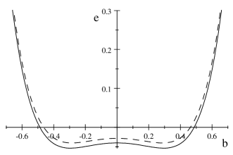
Figure 9: The $1+1$ space-time dimensions effective potential as a function of the one-point function measured in units of $i$ for $H=-\frac{1}{4}\mathtt{,}G=+\frac{1}{2}$ (dashed) and $H=-\frac{1}{2}\mathtt{,}G=-\frac{1}{2}$ (solid) with the stable solution $t=\exp\left(\frac{1}{180H}\left(-60Hb^{2}+6G+6\sqrt{40H^{2}b^{4}+G^{2}-10H}\right)\right)$ of the $\mathcal{PT}$-symmetric $\phi^{6}$ potential .

is the stable one (Fig.9).

In $2+1$ dimensions,  we get $E_{0}(M)-E_{0}(m)=\frac{1}{24\pi}\left(M^{3}-m^{3}\right)$ and $\Delta=\frac{1}{4\pi}\frac{m-M}{\pi}$. Using the parametrization $B=m^{\frac{d-2}{2}}\frac{b}{i\sqrt{\left(4\pi\right)}}$, $g=\left(4\pi\right)Gm^{-d+4}$ , $h=\left(4\pi\right)^{2}Hm^{-2d+6}$ and $M=tm$ we obtain the results;

$$\frac{4\pi E}{m^{3}} =e=-Hb^{6}+\left(15H\left(1-t\right)+G\right)b^{4}-\left(\frac{1}{2}+45H\left(t-1\right)^{2}+6G\left(1-t\right)\right)\allowbreak b^{2}$$

$$+3G\left(t-1\right)^{2}+15H\left(1-t\right)^{3}+\frac{1}{6}\left(t+2\right)\left(t-1\right)^{2},$$

and

$$t =\frac{1}{180H}\left(180H-60Hb^{2}+12G+6\sqrt{40H^{2}b^{4}+4G^{2}-10H}\right),$$

$$t =\frac{1}{180H}\left(180H-60Hb^{2}+12G-6\sqrt{40H^{2}b^{4}+4G^{2}-10H}\right).$$

Only the solution

$$t=\frac{1}{180H}\left(180H-60Hb^{2}+12G+6\sqrt{40H^{2}b^{4}+4G^{2}-10H}\right),$$

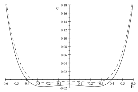
Figure 10: The $2+1$ space-time dimensions effective potential as a function of the one-point function measured in units of $i$ for $H=-1\mathtt{,}G=+\frac{1}{2}$ (dashed) and $H=-1{,}G=-\frac{1}{2}$ (solid) with the stable solution $t=\frac{1}{180H}\left(180H-60Hb^{2}+12G+6\sqrt{40H^{2}b^{4}+4G^{2}-10H}\right)$ of the $\mathcal{PT}$-symmetric $\phi^{6}$ potential .

results in a stable effective potential for the bounded from above $\left(-\phi^{6}\right)$  potential (Fig.10).

V comparison of the effective potential predictions with those from the literature

To test our calculations, let us consider the $h=0$ and negative $g$ ( $\mathcal{PT}\emph{-}\phi^{4}$ theory). In this case; Eq.(5) gives;

$$E=\frac{1}{2}M+\frac{1}{2}B^{2}m^{2}-gB^{4}-\frac{3}{4}\frac{g}{M^{2}}+\frac{1}{4M}\left(-12gB^{2}-M^{2}+m^{2}\right).$$ (15)

Then;

$$\frac{\partial E}{\partial B} =\frac{\partial}{\partial B}\left(\frac{1}{2}M+\frac{1}{2}B^{2}m^{2}-gB^{4}-\frac{3}{4}\frac{g}{M^{2}}+\frac{1}{4M}\left(-12gB^{2}-M^{2}+m^{2}\right)\right)$$

$$=-\allowbreak 4gB^{3}+\frac{1}{M}\left(Mm^{2}-6g\right)B$$ (16)

Also, we have the condition

$$\frac{\partial^{2}E}{\partial B^{2}} =\frac{\partial^{2}}{\partial B^{2}}\left(\frac{1}{2}M+\frac{1}{2}B^{2}m^{2}-gB^{4}-\frac{3}{4}\frac{g}{M^{2}}+\frac{1}{4M}\left(-12gB^{2}-M^{2}+m^{2}\right)\right)$$

$$=-12gB^{2}+\frac{1}{M}\left(Mm^{2}-6g\right),$$ (17)

From Eq.(3) and for $B\neq 0$  we get;

$$m^{2}-4gB^{2}-\frac{6g}{M} =0$$

$$m^{2}-12gB^{2}-\frac{6g}{M} =M^{2},$$ (18)

These are exactly Eq.(39) and Eq.(41) in Ref. jonesgr2 where the authors there obtained them using Schwinger-Dyson equations. Note that, there, they used the interaction term $-\frac{g}{4}\phi^{4}$ but we used $-g\phi^{4}$ interaction term which should be taken into account in the comparison between our results and the results in Ref. jonesgr2 . This result shows that the algorithm we use is quite reasonable.

Another test to our calculations can be drawn from the phase structure of the Hermitian $\phi^{6}$ theory (positive $G$ and positive $H$). In fact, we resort to the Hermitian theory as our calculations for the bounded from above $\phi^{6}$ theory represents the first study for this theory. For technical issues, we use the scaled couplings $\alpha=\frac{G}{4!}$ and $\beta=\frac{H}{4!}$ to generate the plots in Fig.12 and Fig. 12. In these figures we plot the effective potential for the Hermitian $(\phi^{6})$ field theory in $1+1$ dimensions. This theory is well known to have a second order phase transition for positive $G$ while the theory does have a first order phase transition for negative $G$ montecarlo . In fact, our calculations agrees well with these facts which it represents a good test for the validity of our calculations.

VI Conclusions

To conclude, we used the canonical quantization method to study non-Hermitian and $\mathcal{PT}$-symmetric field theory. We showed that the algorithm we follow can reproduce the same results obtained in the literature (using Schwinger-Dyson equation) for the $\mathcal{PT}$-symmetric ($-\phi^{4}$) theory. Also, the algorithm we follow produced the known phase structure for the Hermitian $\phi^{6}$ field theory. We then extended the algorithm to the study of the $\mathcal{PT}$-symmetric ($-\phi^{6}$) theory in $d$ space-time dimensions (for the first time). Regarding this, we calculated the effective potential of the $\mathcal{PT}$-symmetric ($-\phi^{6}$) theory in $d$ space-time dimensions. The classical potential of this theory is bounded from above and thus has not been stressed in the literature due to the believe that this theory is instable. We have shown that as long as the vacuum condensate is imaginary, the effective Hamiltonian is non-Hermitian but $\mathcal{PT}$-symmetric and the effective potential is rather bounded from below which proves the stability of the theory. We found three different vacuum solutions however we figured out that the effective potential is bounded from below for only one vacuum solution out of the three available solutions. In fact, a lesson can be learned from this work because it shows that bounded from above potentials can have both stable and instable vacuum solutions and the bounded from below potentials can have stable as well as instable solutions too. Accordingly, one may expect reflections as well as formation of bound states when incident particles are scattered from either bounded from below or bounded from above potentials. Predictions of such events in the lab will offer a great support to the believe in $\mathcal{PT}$-symmetric theories.

Figure 1: Feynman diagrams contributing to the first order radiative corrections to the vacuum energy of the $\phi^{4}+\phi^{6}$ theory. Diagram (a) generated from the full contraction of the $\psi^{2}$ in the interaction Hamiltonian while diagrams (b) and (c) are generated from the full contraction of the $\psi^{4}$ and $\psi^{6}$ terms in the interaction Hamiltonian, respectively.

.

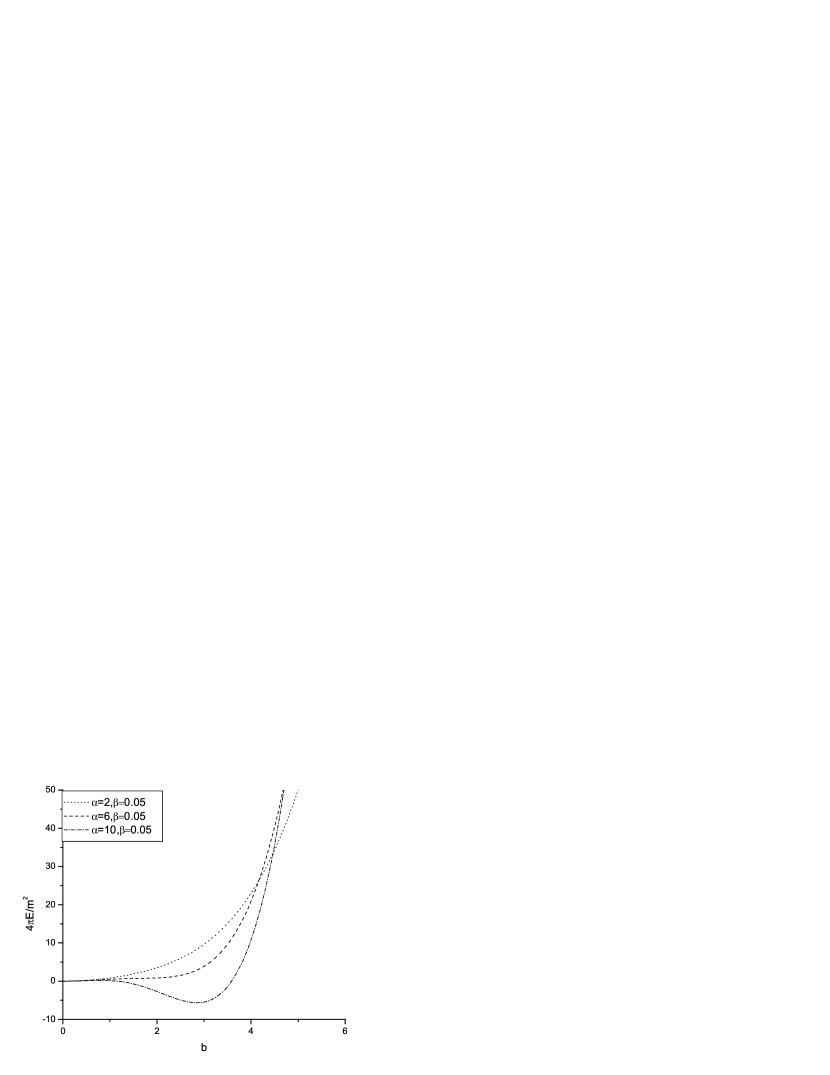
Figure 11: In this figure, we plot the effective potential of the Hermitian $(\phi^{6})_{1+1}$ theory for positive $\alpha=\frac{G}{4!}$ and fixed $\beta=\frac{H}{4!}$. It is clear that the plot shows a second order phase transition which agrees well with the phase structure of the theory in the literature.

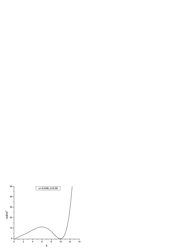
Figure 12: In this figure, we plot the effective potential of the Hermitian $(\phi^{6})_{1+1}$ theory for negative $\alpha=\frac{G}{4!}$ and fixed $\beta=\frac{H}{4!}$. The plot shows a first order phase transition which agrees with the predictions in the literature.

References

• (1) Carl Bender and Stefan Boettcher, Phys.Rev.Lett.80:5243-5246 (1998).
• (2) Abouzeid M. Shalaby and Suleiman S. Al-Thoyaib, Phys. Rev. D 82, 085013 (2010).
• (3) Abouzeid M. Shalaby, Phys.Rev.D 80:025006 (2009).
• (4) Abouzeid Shalaby, Phys.Rev.D 79, 065017 (2009).
• (5) Carl M. Bender, Jun-Hua Chen, and Kimball A. Milton, J.Phys.A39:1657-1668 (2006).
• (6) Abouzeid Shalaby, Int. J. Mod. Phys. A, Vol. 26, No. 17 (2011) 2913–2925.
• (7) A. Mostafazadeh, J. Math. Phys., 43, 3944 (2002).
• (8) A. Mostafazadeh, J. Math. Phys. 43, 205 (2002).
• (9) Carl M. Bender and Philip D. Mannheim, Phys.Rev.Lett.100:110402 (2008).
• (10) Carl M. Bender, Sebastian F. Brandt, Jun-Hua Chen and Qinghai Wang, Phys.Rev. D71, 025014 (2005).
• (11) K. Symanzik, Commun. Math. Phys. 45, 79 (1975).
• (12) C. M. Bender, K. A. Milton, and V. M. Savage, Phys. Rev. D 62, 85001 (2000).
• (13) Frieder Kleefeld, J. Phys. A: Math. Gen. 39 L9–L15 (2006).
• (14) Abouzeid shalaby, Phys.Rev.D76:041702 (2007 ).
• (15) C. M. Bender, D. C. Brody and H. F. Jones, Phys. Rev. Lett. 93, 251601 (2004); Phys. Rev. D70, 025001 (2004).
• (16) Eric S. Swanson, AIP Conf.Proc.1296:75-121, 2010.
• (17) H.F. Jones and R.J. Rivers, Phys.Rev.D74:125022 (2006 ).
• (18) H.F. Jones and R.J. Rivers, Phys. Let. A 373, 3304-3308 (2009).
• (19) H.F. Jones, Int. J. Theor Phys, 50: 1071–1080 ((2011).
• (20) H. F. Jones and J. Mateo, Phys.Rev.D73:085002 (2006 ).
• (21) Michael E. Peskin and Daniel V.Schroeder, An Introduction To Quantum Field Theory (Addison-Wesley Advanced Book Program) ( 1995).
• (22) S.Coleman, Phys.Rev. D11, 2088 (1975).
• (23) Allan M. Din, Phys.Rev.D4, 995 (1971).
• (24) Wen-Fa Lu, Mod.Phys.Lett. A14, 1421-1430 (1999)
• (25) M. Dineykhan, G. V. Efimov, G. Ganbold and S. N. Nedelko, Lect. Notes Phys.  M26, 1 (1995).
• (26) Chang S. J., Phys. Rev. D 12, 1071 (1975).
• (27) Steven. F. Magruder, Phys.Rev. D 14,1602(1976).
• (28) M. Asorey, J.G. Esteve, F. Falceto, J. Salas, Phys. Rev. B52, 9151-9154 (1995).
Refer to caption