Differentiation by integration with Jacobi polynomials

Abstract

In this paper, the numerical differentiation by integration method based on Jacobi polynomials originally introduced by Mboup, Fliess and Join [19, 20] is revisited in the central case where the used integration window is centered. Such a method based on Jacobi polynomials was introduced through an algebraic approach [19, 20] and extends the numerical differentiation by integration method introduced by Lanczos (1956) [21]. The method proposed here, rooted in [19, 20], is used to estimate the $n$th ($n\in\mathbb{N}$) order derivative from noisy data of a smooth function belonging to at least $C^{n+1+q}$ $(q\in\mathbb{N})$. In [19, 20], where the causal and anti-causal cases were investigated, the mismodelling due to the truncation of the Taylor expansion was investigated and improved allowing a small time-delay in the derivative estimation. Here, for the central case, we show that the bias error is $O(h^{q+2})$ where $h$ is the integration window length for $f\in C^{n+q+2}$ in the noise free case and the corresponding convergence rate is $O(\delta^{\frac{q+1}{n+1+q}})$ where $\delta$ is the noise level for a well-chosen integration window length. Numerical examples show that this proposed method is stable and effective.

1 Introduction

Numerical differentiation is concerned with the numerical estimation of derivatives of an unknown function (defined from $\mathbb{R}$ to $\mathbb{R}$) from its noisy measurement data. It has attracted a lot of attention from different points of view: observer design in the control literature [1, 2, 3], digital filter in signal processing [4, 5], the Volterra integral equation of the first kind [6, 7] and identification [8, 9]. The problem of numerical differentiation is ill-posed in the sense that a small error in measurement data can induce a large error in the approximate derivatives. Therefore, various numerical methods have been developed to obtain stable algorithms more or less sensitive to additive noise. They mainly fall into five categories: the finite difference methods [10, 11, 12], the mollification methods [13, 14, 15], the regularization methods [16, 17, 18], the algebraic methods [19, 20] that are the roots of the results reported here and the differentiation by integration methods [21, 22, 23], i.e. using the Lanczos generalized derivatives.

The Lanczos generalized derivative $D_{h}f$, defined in [21] by

$$D_{h}f(x)=\frac{3}{2h^{3}}\int_{-h}^{h}t\,f(x+t)\,dt=\frac{3}{2h}\int_{-1}^{1}t\,f(x+ht)\,dt,$$

is an approximation to the first derivative of $f$ in the sense that $D_{h}f(x)=f^{\prime}\left(x\right)+O(h^{2})$. It is aptly called a method of differentiation by integration. Rangarajana and al. [22] generalized it for higher order derivatives with

$$D_{h}^{(n)}f(x)=\frac{1}{h^{n}}\int_{-1}^{1}\gamma_{n}L_{n}(t)\,f(x+ht)\,dt,\ n\in\mathbb{N},$$

where $f$ is assumed to belong to $C^{n+2}(I)$ with $I$ being an open interval of $\mathbb{R}$ and $L_{n}$ is the $n$th order Legendre polynomial. The coefficient $\gamma_{n}$ is equal to $\frac{1\times 3\times 5\times\cdots\times(2n+1)}{2}$ and $2h>0$ is the length of the integral window on which the estimates are calculated. By applying the scalar product of the Taylor expansion of $f$ at $x$ with $L_{n}$ they showed that $D_{h}^{(n)}f(x)=f^{(n)}(x)+O(h^{2})$. Recently, by using Richardson extrapolation Wang and al. [23] have improved the convergence rate for obtaining high order Lanczos derivatives with the following affine schemes for any $n\in\mathbb{N}$

$$D_{h,\lambda_{n}}^{(n)}f(x)=\frac{1}{h^{n}}\int_{-1}^{1}L_{n}(t)\left(a_{n}\,f(x+ht)+b_{n}\,f(x+\lambda_{n}ht)\right)dt,$$

where $f$ is assumed to belong to $C^{n+4}(I)$, $a_{n}$, $b_{n}$ and $\lambda_{n}$ are chosen such that $D_{h,\lambda_{n}}^{(n)}f(x)=f^{(n)}(x)+O(h^{4})$.

Very recently an algebraic setting for numerical differentiation of noisy signals was introduced in [24] and analyzed in [19, 20]. The reader may find additional theoretical foundations in [25, 26]. The algebraic manipulations used in [19, 20] are inspired by the one used in the algebraic parametric estimation techniques [27, 28, 29]. Let us recall that [19, 20] analyze a causal and an anti-causal version of numerical differentiation by integration method based on Jacobi polynomials

$$D_{h}^{(n)}f(x)=\frac{1}{(\pm h)^{n}}\int_{0}^{1}\gamma_{\kappa,\mu,n}\frac{d^{n}}{dt^{n}}\left\{t^{\kappa+n}(1-t)^{\mu+n}\right\}\,f(x\pm ht)\,dt,\ n\in\mathbb{N},$$

where $f$ is assumed to belong to $C^{n}(I)$ with $I$ being an open interval of $\mathbb{R}$. The coefficient $\gamma_{\kappa,\mu,n}$ is equal to $(-1)^{n}\frac{(\mu+\kappa+2n+1)!}{(\mu+n)!(\kappa+n)!}$, where $\kappa,\mu$ are two integer parameters and $h>0$ is the length of the integral window on which the estimates are calculated. In [19] the authors show that the mismodelling due to the truncation of the Taylor expansion is improved allowing small time-delay in the derivative estimation. Here in this article, we propose to extend these differentiation by integration methods by using as in [19, 20] Jacobi polynomials: for this we use a central estimator (the integration window is now $[-1,1]$) and the design parameters are now allowed to be reals which are strictly greater than $-1$. It is worth to mention that in most of the practical applications the noise can be seen as an integrable bounded function (which noise level is $\delta$ as is considered in this paper). Another point of view concerning the noise definition/characterization is given in [25] for which unbounded noise may appear. Let us mention that the Legendre polynomials are one particular class of Jacobi polynomials, that were used in [22] and [23] to obtain higher order derivative estimations. Moreover, it can be seen that these so obtained derivative estimators correspond to truncated terms in the Jacobi orthogonal series. In fact, the choice of the Jacobi polynomials comes from algebraic manipulations introduced in the recent papers by M. Mboup, C. Join and M. Fliess [19, 20], where the derivative estimations were given by some parameters in the causal and anti-causal cases. Here, we give the derivative estimations in the central case with the same but extended parameters used in [19, 20]. If $f\in C^{n+q+2}$ then we show that the bias error is $O(h^{q+2})$ in the noise free case (where $2h$ is the integration window length). We also show that the corresponding convergence rate is $O(\delta^{\frac{q+1}{n+1+q}})$ for a well-chosen integration window length in the noisy case, where $\delta$ is the noise level. One can see that the obtained causal estimators in [19, 20] are well suited for on-line estimation (which is of importance in signal processing, automatic control, etc.) whereas here the proposed central estimators are only suited for off-line applications. Let us emphasize that those techniques exhibit good robustness properties with respect to corrupting noises (see [25, 30] for more theoretical details). These robustness properties have already been confirmed by numerous computer simulations and several laboratory experiments. Hence, the robustness of the derivative estimators presented in this paper can be ensured as shown by the results and simulations reported here.

This paper is organized as follows: in Section 2 firstly a family of central estimators of the derivatives for higher orders are introduced by using the $n$th order Jacobi polynomials. The corresponding convergence rate is $O(h)$ and can be improved to $O(h^{2})$ when the Jacobi polynomials are ultraspherical polynomials (see [31]). Secondly, a new family of estimators are given. They can be written as an affine combination of the estimators proposed previously. Consequently, we show that if $f\in C^{n+1+q}(I)$ with $q\in\mathbb{N}$ the corresponding convergence rate is improved to $O(h^{q+1})$. Moreover, when the Jacobi polynomials are ultraspherical polynomials, if $f\in C^{n+2+q}(I)$ for any even integer $q$ the corresponding convergence rate can be improved to $O(h^{q+2})$. Numerical tests are given in Section 3 to verify the efficiency and the stability of the proposed estimators.

2 Derivative estimations by using Jacobi orthogonal series

Let $f^{\delta}=f+\varpi$ be a noisy function defined in an open interval $I\subset\mathbb{R}$, where $f\in C^{n+1}(I)$ with $n\in\mathbb{N}$ and the noise $\varpi$ is bounded and integrable with a noise level $\delta$, $i.e.$ $\delta=\displaystyle\sup_{x\in I}|\varpi(x)|$. Contrary to [22] where the $n$th order Legendre polynomials were used, we propose to use, as in [19, 20], the $n$th order Jacobi polynomial so as to obtain estimates of the $n$th order derivative of $f$. The $n$th order Jacobi polynomials (see [31]) are defined as follows

$$P_{n}^{(\alpha,\beta)}(t)=\displaystyle\sum_{j=0}^{n}\binom{n+\alpha}{j}\binom{n+\beta}{n-j}\left(\frac{t-1}{2}\right)^{n-j}\left(\frac{t+1}{2}\right)^{j}$$ (1)

where $\alpha,\beta\in]-1,+\infty[$. Let us denote $\forall g_{1},\,g_{2}\in C^{0}([-1,1])$, $\left\langle g_{1}(\cdot),g_{2}(\cdot)\right\rangle_{\alpha,\beta}=\int_{-1}^{1}w_{\alpha,\beta}(t)g_{1}(t)g_{2}(t)dt$, where $w_{\alpha,\beta}(t)=(1-t)^{\alpha}(1+t)^{\beta}$ is the weight function. Hence, we can denote its associated norm by $\|\cdot\|_{\alpha,\beta}$.

We assume in this article that the parameter $h>0$ and we denote $I_{h}:=\left\{x\in I;\left[x-h,x+h\right]\subset I\right\}$.

2.1 Minimal estimators

In this subsection, let us ignore the noise $\varpi$ for a moment. Then we can define a family of central estimators of $f^{(n)}$.

Proposition 2.1

Let $f\in C^{n+1}(I)$, then a family of central estimators of $f^{(n)}$ can be given as follows

$$\forall x\in I_{h},\ D_{h,\alpha,\beta}^{(n)}f(x)=\frac{1}{h^{n}}\int_{-1}^{1}\rho_{n,\alpha,\beta}(t)\,f(x+ht)dt,$$ (2)

where $\rho_{n,\alpha,\beta}(t)=\frac{2^{-(n+\alpha+\beta+1)}n!}{B(n+\alpha+1,n+\beta+1)}P_{n}^{(\alpha,\beta)}(t)\,w_{\alpha,\beta}(t)$ with $B(n+\alpha+1,n+\beta+1)=\frac{\Gamma(n+\alpha+1)\,\Gamma(n+\beta+1)}{\Gamma(2n+\alpha+\beta+2)}$.

Moreover, we have $D_{h,\alpha,\beta}^{(n)}f(x)=f^{(n)}(x)+O(h)$.

Remark 1

In order to compute $\rho_{n,\alpha,\beta}$, we should calculate $P_{n}^{(\alpha,\beta)}$ whose computational complexity is $O(n^{2})$. Hence, the computational effort of $\rho_{n,\alpha,\beta}$ is $O(n^{2})$.

Proof. By taking the Taylor expansion of $f$, we obtain for any $x\in I_{h}$ that there exists $\theta\in]x-h,x+h[$ such that

$$f(x+ht)=f(x)+htf^{\prime}(x)+\cdots+\frac{h^{n}t^{n}}{n!}f^{(n)}(x)+\frac{h^{n+1}t^{n+1}}{(n+1)!}f^{(n+1)}(\theta).$$ (3)

Substituting $(\ref{Taylor})$ in $(\ref{d_h})$, we deduce from the classical orthogonal properties of the Jacobi polynomials (see [31]) that

$$\int_{-1}^{1}\rho_{n,\alpha,\beta}(t)\,t^{m}\,dt=0,\ 0\leq m<n,$$ (4)

$$\int_{-1}^{1}\rho_{n,\alpha,\beta}(t)\,t^{n}\,dt=(n!).$$ (5)

Using $(\ref{Taylor})$, $(\ref{zero})$ and $(\ref{n!})$, we can conclude that

$$D_{h,\alpha,\beta}^{(n)}f(x)=\frac{1}{h^{n}}\int_{-1}^{1}\rho_{n,\alpha,\beta}(t)\,f(x+ht)dt=f^{(n)}(x)+O(h).$$

Hence, this proof is completed. $\Box$

In fact, we have taken an $n$th order truncation in the Taylor expansion of $f$ in Proposition 2.1 where $n$ is the order of the estimated derivative. Thus, we call these estimators minimal estimators (see [19, 20]). Then, we can deduce the following corollary.

Corollary 2.2

Let $f\in C^{n+1}(I)$, then by assuming that there exists $M_{n+1}>0$ such that for any $x\in I$, $\left|f^{(n+1)}(x)\right|\leq M_{n+1}$, we have

$$\left\|D_{h,\alpha,\beta}^{(n)}f(x)-f^{(n)}(x)\right\|_{\infty}\leq C_{1}h,$$ (6)

where $C_{1}=\frac{M_{n+1}}{(n+1)!}\int_{-1}^{1}|t^{n+1}\rho_{n,\alpha,\beta}(t)|\,dt$.

When $\alpha=\beta$ the Jacobi polynomials are called ultraspherical polynomials (see [31]). In this case, we can improve the convergence rate to $O(h^{2})$ by using the following lemma.

Lemma 2.3

Let $P_{n}^{(\alpha,\alpha)}$ be the $n$th order ultraspherical polynomials, then we have

$$\int_{-1}^{1}P_{n}^{(\alpha,\alpha)}(t)w_{\alpha,\alpha}(t)\,t^{n+l}\,dt=0,$$ (7)

where $l$ is an odd integer.

Proof. Recall the Rodrigues formula (see [31])

$$P_{n}^{(\alpha,\beta)}(t)w_{\alpha,\beta}(t)=\frac{(-1)^{n}}{2^{n}n!}\frac{d^{n}}{dt^{n}}[w_{\alpha+n,\beta+n}(t)],$$ (8)

we get, by substituting $(\ref{rodrigues})$ in $(\ref{zero2})$ and applying $n$ times integrations by parts, that

$$\int_{-1}^{1}P_{n}^{(\alpha,\beta)}(t)w_{\alpha,\beta}(t)\,t^{n+l}\,dt=\frac{(n+l)!}{2^{n}(n!)^{2}}\int_{-1}^{1}w_{\alpha+n,\beta+n}(t)\,t^{l}\,dt.$$ (9)

If $\alpha=\beta$ and $l$ is an odd number then $w_{\alpha+n,\beta+n}(t)\,t^{l}$ is an odd function and the integral in $(\ref{zero3})$ is equal to zero. Hence, this proof is completed. $\Box$

Consequently, we can deduce from Proposition 2.1 and Lemma 2.3 the following corollary.

Corollary 2.4

Let $f\in C^{n+2}(I)$ and $\alpha=\beta$ in Proposition 2.1, then we obtain

$$\forall x\in I_{h},\ D_{h,\alpha,\alpha}^{(n)}f(x)=f^{(n)}(x)+O(h^{2}).$$ (10)

Moreover, if we assume that there exists ${M}_{n+2}>0$ such that for any $x\in I$, $\left|f^{(n+2)}(x)\right|\leq{M}_{n+2}$, then we have

$$\left\|D_{h,\alpha,\alpha}^{(n)}f(x)-f^{(n)}(x)\right\|_{\infty}\leq\hat{C}_{1}h^{2},$$ (11)

where $\hat{C}_{1}=\frac{{M}_{n+2}}{(n+2)!}\int_{-1}^{1}|t^{n+2}\rho_{n,\alpha,\alpha}(t)|\,dt$.

We can see in the following proposition the relation between minimal estimators of $f$ and minimal estimators of $f^{(n)}$.

Proposition 2.5

Let $f\in C^{n+1}(I)$, then we have

$$\forall x\in I_{h},\ D_{h,\alpha,\beta}^{(n)}f(x)=\frac{1}{(2h)^{n}}\frac{\Gamma(\alpha+\beta+2n+2)}{\Gamma(\alpha+\beta+n+2)}\sum_{j=0}^{n}(-1)^{n+j}\binom{n}{j}\ D_{h,\alpha_{n,j},\beta_{j}}^{(0)}f(x),$$ (12)

where $\alpha_{n,j}=\alpha+n-j$ and $\beta_{j}=\beta+j$.

In order to prove this proposition, we give the following lemma.

Lemma 2.6

For any $i\in\mathbb{N}$, we have

$$\forall x\in I_{h},\ \frac{\left\langle P_{i}^{(\alpha,\beta)}(t),f(x+ht)\right\rangle_{\alpha,\beta}}{\|P_{i}^{(\alpha,\beta)}\|^{2}_{\alpha,\beta}}=\sum_{j=0}^{i}(-1)^{i+j}\binom{i}{j}\frac{2i+\alpha+\beta+1}{i+\alpha+\beta+1}\ D_{h,\alpha_{i,j},\beta_{j}}^{(0)}f(x),$$ (13)

where $\alpha_{i,j}=\alpha+i-j$ and $\beta_{j}=\beta+j$.

Proof. Observe from the expression of the Jacobi polynomials given in $(\ref{jacobi})$ that

$$P_{i}^{(\alpha,\beta)}(t)\,w_{\alpha,\beta}(t)=\frac{1}{(-2)^{i}}\sum_{j=0}^{i}\binom{i+\alpha}{j}\binom{i+\beta}{i-j}(-1)^{j}w_{\alpha_{i,j},\beta_{j}}(t),$$ (14)

we get

$$\begin{split}{\left\langle P_{i}^{(\alpha,\beta)}(t),f(x+ht)\right\rangle_{\alpha,\beta}}=&\frac{1}{(-2)^{i}}\sum_{j=0}^{i}\binom{i+\alpha}{j}\binom{i+\beta}{i-j}(-1)^{j}\int_{-1}^{1}w_{\alpha_{i,j},\beta_{j}}(t)\,f(x+ht)\,dt.\end{split}$$ (15)

Then, by using Proposition 2.1 with $n=0$ and $P_{0}^{(\alpha_{i,j},\beta_{j})}(t)\equiv 1$ we obtain

$$\begin{split}\frac{\left\langle P_{i}^{(\alpha,\beta)}(t),f(x+ht)\right\rangle_{\alpha,\beta}}{\|P_{i}^{(\alpha,\beta)}\|^{2}_{\alpha,\beta}}=&\sum_{j=0}^{i}\binom{i+\alpha}{j}\binom{i+\beta}{i-j}\frac{(-1)^{j}}{(-2)^{i}}\frac{B(\alpha_{i,j}+1,\beta_{j}+1)2^{\alpha_{i,j}+\beta_{j}+1}}{\|P_{i}^{(\alpha,\beta)}\|^{2}_{\alpha,\beta}}D^{(0)}_{h,\alpha_{i,j},\beta_{j}}f(x).\end{split}$$ (16)

Recall that (see [31])

$$\|P_{i}^{\left(\alpha,\beta\right)}\|^{2}_{\alpha,\beta}=\frac{2^{\alpha+\beta+1}}{2i+\alpha+\beta+1}\frac{\Gamma(\alpha+i+1)\Gamma(\beta+i+1)}{\Gamma(\alpha+\beta+i+1)\Gamma(i+1)},$$ (17)

then the proof is completed by using $(\ref{norm})$ in $(\ref{pro})$. $\Box$

Proof of Proposition 2.5. From (2), it is easy to show after some calculations that

$$D_{h,\alpha,\beta}^{(n)}f(x)=\frac{1}{(2h)^{n}}\frac{\Gamma(\alpha+\beta+2n+1)}{\Gamma(\alpha+\beta+n+1)}\frac{\left\langle P_{n}^{(\alpha,\beta)}(t),f(x+ht)\right\rangle_{\alpha,\beta}}{\|P_{n}^{(\alpha,\beta)}\|^{2}_{\alpha,\beta}}.$$ (18)

Hence, this proof can be completed by using Lemma 2.6 and $(\ref{relation2})$. $\Box$

Now, we can see in the following proposition that the estimates given in Proposition 2.1 are also equal to the first term in the Jacobi orthogonal series expansion of $f^{(n)}(x+ht)$ at point $t=0$.

Proposition 2.7

Let $f\in C^{n+1}(I)$, then the minimal estimators of $f^{(n)}$ given in Proposition 2.1 can be also written as follows

$$\forall x\in I_{h},\ D_{h,\alpha,\beta}^{(n)}f(x)=\frac{\left\langle P_{0}^{(\alpha+n,\beta+n)}(t),f^{(n)}(x+ht)\right\rangle_{\alpha+n,\beta+n}}{\|P_{0}^{(\alpha+n,\beta+n)}\|^{2}_{\alpha+n,\beta+n}}\ P_{0}^{(\alpha+n,\beta+n)}(0).$$ (19)

Moreover, we have

$$\forall x\in I_{h},\ D_{h,\alpha,\beta}^{(n)}f(x)=D_{h,\alpha+n,\beta+n}^{(0)}f^{(n)}(x).$$ (20)

Proof. By using the Rodrigues formula in $(\ref{d_h})$ and applying $n$ times integrations by parts we get

$$\begin{split}D_{h,\alpha,\beta}^{(n)}f(x)&=\frac{1}{h^{n}}\frac{(-1)^{n}2^{-(2n+\alpha+\beta+1)}}{B(n+\alpha+1,n+\beta+1)}\int_{-1}^{1}\frac{d^{n}}{dt^{n}}[w_{\alpha+n,\beta+n}(t)]\,f(x+ht)\,dt\\ &=\frac{2^{-(2n+\alpha+\beta+1)}}{B(n+\alpha+1,n+\beta+1)}\int_{-1}^{1}w_{\alpha+n,\beta+n}(t)\,f^{(n)}(x+ht)\,dt\\ &=D_{h,\alpha+n,\beta+n}^{(0)}f^{(n)}(x).\end{split}$$

Then, by using $P_{0}^{(\alpha+n,\beta+n)}(t)\equiv 1$ and $\|P_{0}^{(\alpha+n,\beta+n)}\|^{2}_{\alpha+n,\beta+n}=2^{2n+\alpha+\beta+1}{B(n+\alpha+1,n+\beta+1)}$, we can achieve this proof.

$\Box$

2.2 Affine estimators

It is shown in Proposition 2.7 that the minimal estimators of $f^{(n)}(x)$ given in Proposition 2.1 are equal to the value of the $0$ order truncated Jacobi orthogonal series expansion of $f^{(n)}(x+ht)$ at $t=0$. Let us assume that $f\in C^{n+1}(I)$, then we define now the $q$th ($q\in\mathbb{N}$) order truncated Jacobi orthogonal series of $f^{(n)}(x+ht)$ by the following operator

$$\forall x\in I_{h},\ D_{h,\alpha,\beta,q}^{(n)}f(x+th):=\sum_{i=0}^{q}\frac{\left\langle P_{i}^{(\alpha+n,\beta+n)}(\cdot),f^{(n)}(x+h\cdot)\right\rangle_{\alpha+n,\beta+n}}{\|P_{i}^{(\alpha+n,\beta+n)}\|^{2}_{\alpha+n,\beta+n}}\ P_{i}^{(\alpha+n,\beta+n)}(t).$$ (21)

Take $t=0$ in $(\ref{orthogonal_series})$, we obtain a family of estimators of $f^{(n)}(x)$ with

$$\forall x\in I_{h},\ D_{h,\alpha,\beta,q}^{(n)}f(x)=\sum_{i=0}^{q}\frac{\left\langle P_{i}^{(\alpha+n,\beta+n)}(\cdot),f^{(n)}(x+h\cdot)\right\rangle_{\alpha+n,\beta+n}}{\|P_{i}^{(\alpha+n,\beta+n)}\|^{2}_{\alpha+n,\beta+n}}\ P_{i}^{(\alpha+n,\beta+n)}(0).$$ (22)

To better explain our method, let us recall some well-known facts. We consider the subspace of $C^{0}([-1,1])$, defined by

$$\mathcal{H}_{q}=\text{span}\left\{P_{0}^{(\alpha+n,\beta+n)},P_{1}^{(\alpha+n,\beta+n)},\cdots,P_{q}^{(\alpha+n,\beta+n)}\right\}.$$ (23)

Equipped with the inner product $\left\langle\cdot,\cdot\right\rangle_{\alpha+n,\beta+n}$, $\mathcal{H}_{q}$ is clearly a reproducing kernel Hilbert space [32], [33], with the reproducing kernel

$$\mathcal{K}_{q}(\tau,t)=\sum_{i=0}^{q}\frac{P_{i}^{(\alpha+n,\beta+n)}(\tau)P_{i}^{(\alpha+n,\beta+n)}(t)}{\|P_{i}^{(\alpha+n,\beta+n)}\|^{2}_{\alpha+n,\beta+n}}.$$ (24)

The reproducing property implies that for any function $f^{(n)}(x+h\cdot)$ belonging to $C^{0}([-1,1])$, we have

$$\left\langle\mathcal{K}_{q}(\cdot,t),f^{(n)}(x+h\cdot)\right\rangle_{\alpha+n,\beta+n}=D_{h,\alpha,\beta,q}^{(n)}f(x+th),$$ (25)

where $D_{h,\alpha,\beta,q}^{(n)}f(x+h\cdot)$ stands for the orthogonal projection of $f^{(n)}(x+h\cdot)$ on $\mathcal{H}_{q}$. Thus, the estimators given in $(\ref{d_h_N})$ can be obtained by taking $t=0$.

We will see in the following proposition that the estimators $D_{h,\alpha,\beta,q}^{(n)}f(x)$ can be written as an affine combination of different minimal estimators. These estimators are called affine estimators as in [19].

Proposition 2.8

Let $f\in C^{n+1}(I)$, then we have

$$\forall x\in I_{h},\ D_{h,\alpha,\beta,q}^{(n)}f(x)=\sum_{i=0}^{q}{P_{i}^{(\alpha+n,\beta+n)}(0)}\frac{2i+\alpha+\beta+2n+1}{i+\alpha+\beta+2n+1}\sum_{j=0}^{i}(-1)^{i+j}\binom{i}{j}D_{h,\alpha_{i,j},\beta_{j}}^{(n)}f(x),$$ (26)

where $q\in\mathbb{N}$, $\alpha_{i,j}=\alpha+i-j$ and $\beta_{j}=\beta+j$. Moreover, we have

$$\sum_{i=0}^{q}{P_{i}^{(\alpha+n,\beta+n)}(0)}\frac{2i+\alpha+\beta+2n+1}{i+\alpha+\beta+2n+1}\sum_{j=0}^{i}(-1)^{i+j}\binom{i}{j}=1.$$ (27)

Proof. By replacing $\alpha$ by $\alpha+n$, $\beta$ by $\beta+n$ and $f(x+ht)$ by $f^{(n)}(x+ht)$ in Lemma 2.6, we obtain

$$\frac{\left\langle P_{i}^{(\alpha+n,\beta+n)}(t),f^{(n)}(x+ht)\right\rangle_{\alpha+n,\beta+n}}{\|P_{i}^{(\alpha+n,\beta+n)}\|^{2}_{\alpha+n,\alpha+n}}=\sum_{j=0}^{i}(-1)^{i+j}\binom{i}{j}\frac{2i+\alpha+\beta+2n+1}{i+\alpha+\beta+2n+1}\ D_{h,\alpha_{i,j}+n,\beta_{j}+n}^{(0)}f^{(n)}(x).$$ (28)

Then $(\ref{affine_relation})$ can be obtained by using $(\ref{equalite})$ and $(\ref{d_h_N})$. By using the Binomial relation, $(\ref{affine_sum})$ can be easily obtained. $\Box$

Hence, by using Proposition 2.1 an explicit formulation of these affine estimators is obtained in the following corollary.

Corollary 2.9

Let $f\in C^{n+1}(I)$, then the affine estimators of $f^{(n)}$ can be written as

$$\forall x\in I_{h},\ D_{h,\alpha,\beta,q}^{(n)}f(x)=\frac{1}{h^{n}}\int_{-1}^{1}Q_{\alpha,\beta,n,q}(t)\,f(x+ht)\,dt,$$ (29)

where

$$Q_{\alpha,\beta,n,q}(t)=\displaystyle\sum_{i=0}^{q}{P_{i}^{(\alpha+n,\beta+n)}(0)}\sum_{j=0}^{i}(-1)^{i+j}\binom{i}{j}\frac{2i+\alpha+\beta+2n+1}{i+\alpha+\beta+2n+1}\,\rho_{n,\alpha_{i,j},\beta_{j}}(t)$$ (30)

with $q\in\mathbb{N}$, $\rho_{n,\alpha_{i,j},\beta_{j}}$ given in Proposition 2.1 and $\alpha_{i,j}=\alpha+i-j$, $\beta_{j}=\beta+j$.

Consequently these affine estimators are also differentiation by integration estimators.

Remark 2

$Q_{\alpha,\beta,n,q}$ is a sum of $\frac{1}{2}(q+1)(q+2)$ terms. According to Remark 1, the computational effort of each term is $O(n^{2})$. Hence, the computational effort of $Q_{\alpha,\beta,n,q}$ is also $O(n^{2})$.

It is shown in Proposition 2.1 that the convergence rate of minimal estimators is $O(h)$. We will see in the following proposition that the convergence rate of affine estimators can be improved to $O(h^{q+1})$.

Proposition 2.10

Let $f\in C^{n+1+q}(I)$ with $q\in\mathbb{N}$, then we have

$$\forall x\in I_{h},\ D_{h,\alpha,\beta,q}^{(n)}f(x)=f^{(n)}(x)+O(h^{q+1}).$$ (31)

Moreover, if we assume that there exists $M_{n+1+q}>0$ such that for any $x\in I$, $\left|f^{(n+1+q)}(x)\right|\leq M_{n+1+q}$, then we have

$$\left\|D_{h,\alpha,\beta,q}^{(n)}f(x)-f^{(n)}(x)\right\|_{\infty}\leq C_{2}h^{q+1},$$ (32)

where $C_{2}=\frac{M_{n+1+q}}{(n+1+q)!}\int_{-1}^{1}|t^{n+1+q}Q_{\alpha,\beta,n,q}(t)|\,dt$.

Proof. By taking the Taylor expansion of $f$, we get for any $x\in I_{h}$ there exists $\xi\in]x-h,x+h[$ such that

$$f(x+ht)=f_{n+q}(x+ht)+\frac{h^{n+1+q}t^{n+1+q}}{(n+1+q)!}f^{(n+1+q)}(\xi),$$ (33)

where $f_{n+q}(x+ht)=\displaystyle\sum_{j=0}^{n+q}\frac{h^{j}t^{j}}{j!}f^{(j)}(x)$ is the $(n+q)$th order truncated Taylor series expansion of $f(x+ht)$.

Let us take the Jacobi orthogonal series expansion of $f_{n+q}^{(n)}(x+ht)$. Then by taking $t=0$, we obtain

$$\begin{split}f_{n+q}^{(n)}(x)=&\sum_{i=0}^{q}\frac{\left\langle P_{i}^{(\alpha+n,\beta+n)}(t),f_{n+q}^{(n)}(x+ht)\right\rangle_{\alpha+n,\beta+n}}{\|P_{i}^{(\alpha+n,\beta+n)}\|^{2}_{\alpha+n,\alpha+n}}\ P_{i}^{(\alpha+n,\beta+n)}(0).\end{split}$$ (34)

Similarly to $(\ref{d_h_N})$ we obtain

$$f_{n+q}^{(n)}(x)=\frac{1}{h^{n}}\int_{-1}^{1}Q_{\alpha,\beta,n,{q}}(t)f_{n+q}(x+ht)dt,$$ (35)

from $(\ref{D_h_N})$ where $Q_{\alpha,\beta,n,q}$ is given in Corollary 2.9 by $(\ref{Q})$.

By calculating the value of the $n$th order derivative of $f_{n+q}^{(n)}$ at $t=0$, we obtain $f_{n+q}^{(n)}(x)=f^{(n)}(x)$. Then by using $(\ref{D_h_N})$ and $(\ref{f_N})$ we obtain

$$\begin{split}D_{h,\alpha,\beta,{q}}^{(n)}f(x)-f^{(n)}(x)=&\frac{1}{h^{n}}\int_{-1}^{1}Q_{\alpha,\beta,n,q}(t)\left[f(x+ht)-f_{n+q}(x+ht)\right]dt\\ =&\frac{h^{q+1}}{(n+1+q)!}\int_{-1}^{1}Q_{\alpha,\beta,n,q}(t)t^{n+1+q}f^{(n+1+q)}(\xi)dt\\ =&O(h^{q+1}).\end{split}$$

Consequently, if for any $x\in I$ $\left|f^{(n+1+q)}(x)\right|\leq M_{n+1+q}$, then we have

$$\left\|D_{h,\alpha,\beta,{q}}^{(n)}f(x)-f^{(n)}(x)\right\|_{\infty}\leq h^{q+1}\frac{M_{n+1+q}}{(n+1+q)!}\int_{-1}^{1}|t^{n+1+q}Q_{\alpha,\beta,n,q}(t)|\,dt.$$

$\Box$

We can deduce that the affine estimator for $f^{(n)}(x)$ obtained by taking the $q$th order truncated Jacobi orthogonal series expansion of $f^{(n)}(x+h\cdot)$ can be also obtained by taking the $(n+q)$th order truncated Taylor series expansion of $f$ with a scalar product of Jacobi polynomials.

Moreover, let $f_{n+q}(x+ht)=f_{n}(x+ht)+r_{q}(x+ht)$ where $r_{q}(x+ht)=\displaystyle\sum_{j=n+1}^{n+q}\frac{h^{j}t^{j}}{j!}f^{(j)}(x)$ for $q\geq 1$ and $r_{q}(x+ht)=0$ for $q=0$, then $(\ref{f_q})$ becomes

$$f_{n+q}^{(n)}(x)=\sum_{i=0}^{q}\frac{\left\langle P_{i}^{(\alpha+n,\beta+n)}(t),f_{n}^{(n)}(x+ht)\right\rangle_{\alpha+n,\beta+n}}{\|P_{i}^{(\alpha+n,\beta+n)}\|^{2}_{\alpha+n,\alpha+n}}\ P_{i}^{(\alpha+n,\beta+n)}(0)+R,$$

where $R=\displaystyle\sum_{i=0}^{q}\frac{\left\langle P_{i}^{(\alpha+n,\beta+n)}(t),r_{q}^{(n)}(x+ht)\right\rangle_{\alpha+n,\beta+n}}{\|P_{i}^{(\alpha+n,\beta+n)}\|^{2}_{\alpha+n,\alpha+n}}\ P_{i}^{(\alpha+n,\beta+n)}(0)$.

Observe that $f_{n}^{(n)}(x+h\cdot)$ is a $0$th order polynomial, then by using the orthogonal properties of $P_{i}^{(\alpha+n,\beta+n)}$ we have

$$\begin{split}&\sum_{i=0}^{q}\frac{\left\langle P_{i}^{(\alpha+n,\beta+n)}(t),f_{n}^{(n)}(x+ht)\right\rangle_{\alpha+n,\beta+n}}{\|P_{i}^{(\alpha+n,\beta+n)}\|^{2}_{\alpha+n,\alpha+n}}\ P_{i}^{(\alpha+n,\beta+n)}(0)\\ =&\frac{\left\langle P_{0}^{(\alpha+n,\beta+n)}(t),f_{n}^{(n)}(x+ht)\right\rangle_{\alpha+n,\beta+n}}{\|P_{0}^{(\alpha+n,\beta+n)}\|^{2}_{\alpha+n,\alpha+n}}\ P_{0}^{(\alpha+n,\beta+n)}(0)=f_{n}^{(n)}(x).\end{split}$$

By calculating the value of the $n$th order derivative of $f_{n+q}^{(n)}$ and $f_{n}^{(n)}$ at $t=0$, we obtain $f_{n+q}^{(n)}(x)=f_{n}^{(n)}(x)=f^{(n)}(x)$. Hence, we get $R=0$. Hence, we can deduce that

$$R=\frac{1}{h^{n}}\int_{-1}^{1}Q_{\alpha,\beta,n,{q}}(t)r_{q}(x+ht)dt=0,$$ (36)

where $Q_{\alpha,\beta,n,q}$ is given in Corollary 2.9 by $(\ref{Q})$.

Consequently, $(\ref{r})$ explains why the convergence rate can be improved from $O(h)$ to $O(h^{q+1})$: the price to pay is some more smoothness hypotheses on the function $f$.

If we consider the noisy function $f^{\delta}$, then it is sufficient to replace $f(x+h\cdot)$ in $(\ref{D_h_N})$ by $f^{\delta}(x+h\cdot)$ so as to estimate $f^{(n)}(x)$. Then we have the following definition.

Definition 2.11

Let $f^{\delta}=f+\varpi$ be a noisy function, where $f\in C^{n+1}(I)$ and $\varpi$ is a bounded and integrable noise with a noise level $\delta$. Then a family of estimators of $f^{(n)}$ is defined as follows

$$\forall x\in I_{h},\ D_{h,\alpha,\beta,{q}}^{(n)}f^{\delta}(x)=\frac{1}{h^{n}}\int_{-1}^{1}Q_{\alpha,\beta,n,{q}}(t)\,f^{\delta}(x+ht)\,dt,$$ (37)

where $Q_{\alpha,\beta,n,q}$ is given by $(\ref{Q})$.

In the following proposition we study the estimation error for these estimators.

Proposition 2.12

Let $f^{\delta}$ be a noisy function where $f\in C^{n+1+q}(I)$ and $\varpi$ is a bounded and integrable noise with a noise level $\delta$, then

$$\left\|D_{h,\alpha,\beta,{q}}^{(n)}f^{\delta}(x)-f^{(n)}(x)\right\|_{\infty}\leq C_{2}h^{q+1}+C_{3}\frac{\delta}{h^{n}},$$ (38)

where $C_{2}$ is given in Proposition 2.10 and $C_{3}=\int_{-1}^{1}|Q_{\alpha,\beta,n,q}(t)|\,dt.$

Moreover, if we choose $h=\left[\frac{nC_{3}}{(q+1)C_{2}}\delta\right]^{\frac{1}{n+q+1}}$, then we have

$$\left\|D_{h,\alpha,\beta,{q}}^{(n)}f^{\delta}(x)-f^{(n)}(x)\right\|_{\infty}=O(\delta^{\frac{q+1}{n+1+q}}).$$ (39)

Proof. Since

$$\left\|D_{h,\alpha,\beta,{q}}^{(n)}f^{\delta}(x)-D_{h,\alpha,\beta,{q}}^{(n)}f(x)\right\|_{\infty}=\left\|D_{h,\alpha,\beta,{q}}^{(n)}\left[f^{\delta}(x)-f(x)\right]\right\|_{\infty}\leq\frac{\delta}{h^{n}}\int_{-1}^{1}\left|Q_{\alpha,\beta,n,q}(t)\right|\,dt,$$

by using Proposition 2.10 we get

$$\begin{split}\left\|D_{h,\alpha,\beta,{q}}^{(n)}f^{\delta}(x)-f^{(n)}(x)\right\|_{\infty}&\leq\left\|D_{h,\alpha,\beta,{q}}^{(n)}f^{\delta}(x)-D_{h,\alpha,\beta,{q}}^{(n)}f(x)\right\|_{\infty}+\left\|D_{h,\alpha,\beta,{q}}^{(n)}f(x)-f^{(n)}(x)\right\|_{\infty}\\ &\leq C_{2}h^{q+1}+C_{3}\frac{\delta}{h^{n}},\end{split}$$

where $C_{3}=\int_{-1}^{1}|Q_{\alpha,\beta,n,q}(t)|\,dt.$ Let us denote the error bound by $\psi(h)=C_{2}h^{q+1}+C_{3}\frac{\delta}{h^{n}}$. Consequently, we can calculate its minimum value. It is obtained for $h^{\ast}=\left[\frac{nC_{3}}{(q+1)C_{2}}\delta\right]^{\frac{1}{n+q+1}}$ and

$$\psi(h^{\ast})=\frac{n+1+q}{q+1}\left(\frac{q+1}{n}\right)^{\frac{n}{n+1+q}}C_{2}^{\frac{n}{n+1+q}}C_{3}^{\frac{q+1}{n+1+q}}\delta^{\frac{q+1}{n+1+q}}.$$ (40)

Then, the proof is completed. $\Box$

In Proposition 2.8, we improve the convergence rate from $O(h)$ to $O(h^{q+1})$ ($q\in\mathbb{N}$) for the exact function $f$ by taking an affine combination of minimal estimators of $f^{(n)}$. Here, the convergence rate is also improved for noisy functions. It passes from $O(\delta^{\frac{1}{n+1}})$ to $O(\delta^{\frac{q+1}{n+1+q}})$ if we choose $h=c\,\delta^{\frac{1}{n+1+q}}$, where $c$ is a constant.

Remark 3

Usually, the sampling data are given in discrete case. We should use a numerical integration method to approximate the integrals in our estimators. This numerical method will produce a numerical error. Hence, we always set the value of $h$ larger than the optimal one calculated in the previous proof.

We have seen in the previous subsection that the convergence rate of minimal estimators can be improved to $O(h^{2})$ when $\alpha=\beta$. Let us then study the convergence rate of affine estimators in this case.

Corollary 2.13

Let $f\in C^{n+2+q}(I)$ where $q$ is an even integer. If we set $\alpha=\beta$ in (22), then we have

$$\forall x\in I_{h},\ D_{h,\alpha,\alpha,q}^{(n)}f(x)=f^{(n)}(x)+O(h^{q+2}).$$ (41)

Moreover, if we assume that there exists ${M}_{n+2+q}>0$ such that for any $x\in I$, $\left|f^{(n+q+2)}(x)\right|\leq{M}_{n+2+q}$, then we have

$$\left\|D_{h,\alpha,\alpha,q}^{(n)}f(x)-f^{(n)}(x)\right\|_{\infty}\leq\hat{C}_{2}h^{q+2},$$ (42)

where $\hat{C}_{2}=\frac{{M}_{n+2+q}}{(n+q+2)!}\int_{-1}^{1}|t^{n+q+2}Q_{\alpha,n,q}(t)|\,dt$ and

$$Q_{\alpha,n,q}(t)=\displaystyle\sum_{i=0}^{\frac{q}{2}}{P_{2i}^{(\alpha+n,\alpha+n)}(0)}\sum_{j=0}^{2i}(-1)^{j}\binom{2i}{j}\frac{4i+2\alpha+2n+1}{2i+2\alpha+2n+1}\,\rho_{n,\alpha_{2i,j},\beta_{j}}(t)$$ (43)

with $\rho_{n,\alpha_{2i,j},\beta_{j}}$ given in Proposition 2.1 and $\alpha_{2i,j}=\alpha+2i-j$, $\beta_{j}=\alpha+j$.

Proof. Observe that $P_{q+1}^{(\alpha+n,\alpha+n)}(-t)=(-1)^{(q+1)}P_{q+1}^{(\alpha+n,\alpha+n)}(t)$ for any $t\in[-1,1]$ (see [31] p.80), we obtain $P_{q+1}^{(\alpha+n,\alpha+n)}(0)=0$. Hence, $(\ref{d_h_N})$ becomes

$$\begin{split}D_{h,\alpha,\alpha,q}^{(n)}f(x)&=\sum_{i=0}^{q+1}\frac{\left\langle P_{i}^{(\alpha+n,\alpha+n)}(t),f^{(n)}(x+ht)\right\rangle_{\alpha+n,\alpha+n}}{\|P_{i}^{(\alpha+n,\alpha+n)}\|^{2}_{\alpha+n,\alpha+n}}\ P_{i}^{(\alpha+n,\alpha+n)}(0).\end{split}$$

If $f\in C^{n+2+q}(I)$, then let us take $f_{n+q+1}$ as the $(n+q+1)$th order truncated Taylor series expansion of $f(x+ht)$. By taking the Jacobi orthogonal series expansion of $f^{(n)}_{n+q+1}$

$$f^{(n)}_{n+q+1}(x)=\sum_{i=0}^{q+1}\frac{\left\langle P_{i}^{(\alpha+n,\alpha+n)}(t),f^{(n)}_{n+q+1}(x+ht)\right\rangle_{\alpha+n,\alpha+n}}{\|P_{i}^{(\alpha+n,\alpha+n)}\|^{2}_{\alpha+n,\alpha+n}}\ P_{i}^{(\alpha+n,\alpha+n)}(0),$$

we obtain

$$\begin{split}D_{h,\alpha,\alpha,q}^{(n)}f(x)-f^{(n)}(x)&=D_{h,\alpha,\alpha,q}^{(n)}f(x)-f^{(n)}_{n+q+1}(x)\\ &=\sum_{i=0}^{q+1}\frac{\left\langle P_{i}^{(\alpha+n,\alpha+n)}(t),f^{(n)}(x+ht)-f^{(n)}_{n+q+1}(x+ht)\right\rangle_{\alpha+n,\alpha+n}}{\|P_{i}^{(\alpha+n,\alpha+n)}\|^{2}_{\alpha+n,\alpha+n}}\ P_{i}^{(\alpha+n,\alpha+n)}(0)\\ &=\frac{1}{h^{n}}\int_{-1}^{1}Q_{\alpha,\alpha,n,q}(t)\left[f(x+ht)-f_{n+q+1}(x+ht)\right]dt\\ &=\frac{h^{q+2}}{(n+2+q)!}\int_{-1}^{1}Q_{\alpha,\alpha,n,q}(t)t^{n+2+q}f^{(n+2+q)}(\xi^{\prime})dt,\ \ \xi^{\prime}\in]x-h,x+h[\\ &=O(h^{q+2}).\end{split}$$

Consequently, $(\ref{bound})$ follows directly from the hypothesis on $\left|f^{(n+q+2)}(x)\right|$. Since $P_{i}^{(\alpha+n,\alpha+n)}(0)=0$ for any odd integer $i$, $(\ref{Q2})$ can be obtained by using $(\ref{Q})$. Then this proof is completed. $\Box$

Remark 4

According to [34], we can deduce the asymptotic behavior of the number $\xi^{\prime}$ when $h\rightarrow 0^{+}$

$$\lim_{h\rightarrow 0^{+}}\frac{|\xi^{\prime}-x|}{h}=\frac{1}{n+q+3}.$$ (44)

Similarly to Proposition 2.12, we can obtain the following corollary.

Corollary 2.14

Let $f\in C^{n+2+q}(I)$ where $q$ is an even integer. If $\alpha=\beta$ in Definition 2.11, then the estimation error for $D_{h,\alpha,\alpha,{q}}^{(n)}f^{\delta}(x)$ is given by

$$\left\|D_{h,\alpha,\alpha,{q}}^{(n)}f^{\delta}(x)-f^{(n)}(x)\right\|_{\infty}\leq\hat{C}_{2}h^{q+2}+C_{3}\frac{\delta}{h^{n}},$$

where $\hat{C}_{2}$ is given in Corollary 2.13 and $C_{3}$ is given in Proposition 2.12.

Moreover, if we choose $\hat{h}=\left[\frac{nC_{3}}{(q+2)\hat{C}_{2}}\delta\right]^{\frac{1}{n+q+2}}$, then we have

$$\left\|D_{h,\alpha,\alpha,{q}}^{(n)}f^{\delta}(x)-f^{(n)}(x)\right\|_{\infty}=O(\delta^{\frac{q+2}{n+2+q}}).$$

In the following proposition, if we assume that $f\in C^{n-1}(I)$ then we can define the generalized derivative of $f^{(n)}$. We can see that if the right and left hand derivatives for the $n$th order exist, then this generalized derivative converges to the average value of these one-sided derivatives.

Proposition 2.15

Let $f\in C^{n-1}(I)$, then we define the generalized derivative of $f^{(n)}$ by

$$\forall x\in I_{h},\ D_{h,\alpha,\alpha,q}^{(n)}f(x)=\frac{1}{h^{n}}\int_{-1}^{1}Q_{\alpha,n,q}(t)\,f(x+ht)\,dt,$$ (45)

where $Q_{\alpha,n,q}$ is defined by (43). Moreover, if $f^{(n)}_{+}(x)$ and $f^{(n)}_{-}(x)$ exist at any point $x\in I_{h}$, then we have

$$\lim_{h\rightarrow 0^{+}}D_{h,\alpha,\alpha,{q}}^{(n)}f(x)=\frac{1}{2}\left(f^{(n)}_{+}(x)+f^{(n)}_{-}(x)\right),$$ (46)

where $f^{(n)}_{+}$ (resp. $f^{(n)}_{-}$) denotes the right (resp. left) hand derivative for the $n$th order.

Before proving this proposition, let us give the following lemma.

Lemma 2.16

Let $n\in\mathbb{N}$ and $Q_{\alpha,n,q}$ be the function defined on $[-1,1]$ by $(\ref{Q2})$ where $q$ is an even integer. If $n$ is even then $Q_{\alpha,n,q}$ is also even, odd else.

Proof. By taking $\alpha=\beta$ in (22), we obtain

$$\forall x\in I_{h},\ D_{h,\alpha,\alpha,q}^{(n)}f(x)=\sum_{i=0}^{q}\frac{P_{i}^{(\alpha+n,\alpha+n)}(0)}{\|P_{i}^{(\alpha+n,\alpha+n)}\|^{2}_{\alpha+n,\alpha+n}}\int_{-1}^{1}P_{i}^{(\alpha+n,\alpha+n)}(t)w_{\alpha+n,\alpha+n}(t)f^{(n)}(x+ht)dt.$$ (47)

By using (14) and replacing $\alpha,\beta$ by $\alpha+n$, we get for $l=0,\cdots,n-1$

$$\frac{d^{l}}{dt^{l}}\left[P_{i}^{(\alpha+n,\alpha+n)}(t)\,w_{\alpha+n,\alpha+n}(t)\right]=\frac{1}{(-2)^{i}}\sum_{j=0}^{i}\binom{i+\alpha+n}{j}\binom{i+\alpha+n}{i-j}(-1)^{j}\frac{d^{l}}{dt^{l}}\left[w_{\alpha_{i+n,j},\alpha_{j+n}}(t)\right],$$

where $\alpha_{i+n,j}=\alpha+i+n-j$, $\alpha_{j+n}=\alpha+j+n$. Then, by applying the Rodrigues formula, we get

$$\begin{split}&\frac{d^{l}}{dt^{l}}\left[P_{i}^{(\alpha+n,\alpha+n)}(t)\,w_{\alpha+n,\alpha+n}(t)\right]\\ =&\frac{l!}{2^{i-l}}\sum_{j=0}^{i}\binom{i+\alpha+n}{j}\binom{i+\alpha+n}{i-j}(-1)^{j+i+l}P_{n}^{(\alpha_{i+n-l,j},\alpha_{j+n-l})}(t)w_{\alpha_{i+n-l,j},\alpha_{j+n-l}}(t),\end{split}$$

where $\alpha_{i+n-l,j}=\alpha+i+n-j-l$, $\alpha_{j+n-l}=\alpha+j+n-l$. Hence, we get that $\frac{d^{l}}{dt^{l}}[P_{i}^{(\alpha+n,\alpha+n)}\,w_{\alpha+n,\alpha+n}]$ are equal to $0$ at $-1$ and $1$. Thus, by applying $n$ times integrations by parts in $(\ref{d_h_N2})$, we obtain

$$\forall x\in I_{h},\ D_{h,\alpha,\alpha,q}^{(n)}f(x)=\frac{(-1)^{n}}{h^{n}}\sum_{i=0}^{q}\frac{P_{i}^{(\alpha+n,\alpha+n)}(0)}{\|P_{i}^{(\alpha+n,\alpha+n)}\|^{2}_{\alpha+n,\alpha+n}}\int_{-1}^{1}\frac{d^{n}}{dt^{n}}\left[P_{i}^{(\alpha+n,\alpha+n)}(t)w_{\alpha+n,\alpha+n}(t)\right]f(x+ht)dt.$$ (48)

By using Corollary 2.9 with $\alpha=\beta$, we get

$$Q_{\alpha,n,q}(t)=(-1)^{n}\sum_{i=0}^{q}\frac{P_{i}^{(\alpha+n,\alpha+n)}(0)}{\|P_{i}^{(\alpha+n,\alpha+n)}\|^{2}_{\alpha+n,\alpha+n}}\frac{d^{n}}{dt^{n}}\left[P_{i}^{(\alpha+n,\alpha+n)}(t)w_{\alpha+n,\alpha+n}(t)\right].$$ (49)

Since $P_{i}^{(\alpha+n,\alpha+n)}(0)=0$ for any odd integer $i$, (49) becomes

$$Q_{\alpha,n,q}(t)=(-1)^{n}\sum_{i=0}^{\frac{q}{2}}\frac{P_{2i}^{(\alpha+n,\alpha+n)}(0)}{\|P_{2i}^{(\alpha+n,\alpha+n)}\|^{2}_{\alpha+n,\alpha+n}}\frac{d^{n}}{dt^{n}}\left[P_{2i}^{(\alpha+n,\alpha+n)}(t)w_{\alpha+n,\alpha+n}(t)\right].$$ (50)

Since $P_{2i}^{(\alpha+n,\alpha+n)}(-t)=P_{2i}^{(\alpha+n,\alpha+n)}(t)$ (see [31]) and $w_{\alpha+n,\alpha+n}(-t)=w_{\alpha+n,\alpha+n}(t)$, we have

$$\frac{d^{n}}{dt^{n}}\left[P_{2i}^{(\alpha+n,\alpha+n)}(t)w_{\alpha+n,\alpha+n}(t)\right]=(-1)^{n}\frac{d^{n}}{dt^{n}}\left[P_{2i}^{(\alpha+n,\alpha+n)}(-t)w_{\alpha+n,\alpha+n}(-t)\right].$$

Thus, we have $Q_{\alpha,n,q}(t)=(-1)^{n}Q_{\alpha,n,q}(-t)$. Then this proof is completed. $\Box$

Proof of Proposition 2.15. Let us recall the local Taylor formula with the Peano remainder term [35]. For any given $\varepsilon^{\prime}>0$, there exists $\delta>0$ such that

$$\left|f(x+ht)-f_{n-1}(x+ht)-\frac{f_{-}^{(n)}(x)}{n!}(ht)^{n}\right|<\varepsilon^{\prime}|ht|^{n},\text{ for }\delta<ht<0,$$ (51)

and

$$\left|f(x+ht)-f_{n-1}(x+ht)-\frac{f_{+}^{(n)}(x)}{n!}(ht)^{n}\right|<\varepsilon^{\prime}(ht)^{n},\text{ for }0<ht<\delta,$$ (52)

where $f_{n-1}(x+ht)$ is the $(n-1)$th order truncated Taylor series expansion of $f(x+ht)$. Let us consider the function $g(x)=x^{n}$ the $n$th order derivative of which is equal to $(n!)$. Thus, by using (22) we have

$$\forall x\in I_{h},\ D_{h,\alpha,\alpha,q}^{(n)}g(x)=(n!).$$

Thus, by applying Corollary 2.9 with $\alpha=\beta$, we get

$$\forall x\in I_{h},\ D_{h,\alpha,\alpha,q}^{(n)}g(x)=\frac{1}{h^{n}}\int_{-1}^{1}Q_{\alpha,n,q}(t)\,g(x+ht)\,dt=(n!).$$

In particular, by taking $x=0$ we get $\frac{1}{h^{n}}\int_{-1}^{1}Q_{\alpha,n,q}(t)\,(ht)^{n}\,dt=(n!).$ According to Lemma 2.16, $t^{n}Q_{\alpha,n,q}(t)$ with $t\in[-1,1]$ is an odd function. Hence, we have $\frac{1}{h^{n}}\int_{-1}^{0}Q_{\alpha,n,q}(t)\,(ht)^{n}\,dt=\frac{1}{h^{n}}\int_{0}^{1}Q_{\alpha,n,q}(t)\,(ht)^{n}\,dt.$ Thus, we get

$$\frac{1}{h^{n}}\int_{-1}^{0}Q_{\alpha,n,q}(t)\frac{f_{-}^{(n)}(x)}{n!}(ht)^{n}\,dt=\frac{1}{2}f_{-}^{(n)}(x),$$ (53)

and

$$\frac{1}{h^{n}}\int_{0}^{1}Q_{\alpha,n,q}(t)\frac{f_{+}^{(n)}(x)}{n!}(ht)^{n}\,dt=\frac{1}{2}f_{+}^{(n)}(x).$$ (54)

By using (22) and Corollary 2.9 with $\alpha=\beta$ we get

$$\forall x\in I_{h},\ D_{h,\alpha,\alpha,q}^{(n)}f_{n-1}(x)=\frac{1}{h^{n}}\int_{-1}^{1}Q_{\alpha,n,q}(t)\,f_{n-1}(x+ht)\,dt=0.$$ (55)

Hence, by using (53), (54) and (55) we obtain

$$\begin{split}&\left|D_{h,\alpha,\alpha,{q}}^{(n)}f(x)-\frac{1}{2}\left(f^{(n)}_{+}(x)+f^{(n)}_{-}(x)\right)\right|\\ \leq&\frac{1}{h^{n}}\int_{-1}^{0}\left|Q_{\alpha,n,q}(t)\left(f(x+ht)-f_{n-1}(x+ht)-\frac{f_{-}^{(n)}(x)}{n!}(ht)^{n}\right)\right|dt\\ +&\frac{1}{h^{n}}\int_{0}^{1}\left|Q_{\alpha,n,q}(t)\left(f(x+ht)-f_{n-1}(x+ht)-\frac{f_{+}^{(n)}(x)}{n!}(ht)^{n}\right)\right|dt.\end{split}$$ (56)

By using (43), we get

$$\int_{0}^{1}\left|Q_{\alpha,n,q}(t)\right|dt\leq\displaystyle\sum_{i=0}^{\frac{q}{2}}{\left|P_{2i}^{(\alpha+n,\alpha+n)}(0)\right|}\sum_{j=0}^{2i}\binom{2i}{j}\frac{4i+2\alpha+2n+1}{2i+2\alpha+2n+1}\int_{0}^{1}\left|\rho_{n,\alpha_{2i,j},\beta_{j}}(t)\right|dt.$$ (57)

Then, according to (2) and (14) we can obtain that $\int_{0}^{1}\left|\rho_{n,\alpha_{2i,j},\beta_{j}}(t)\right|dt<\infty$. Hence,

$$\int_{0}^{1}\left|Q_{\alpha,n,q}(t)\,t^{n}\right|dt\leq\int_{0}^{1}\left|Q_{\alpha,n,q}(t)\right|dt<\infty.$$

Consequently, for any $\varepsilon>0$, by using (LABEL:inegalite), (51) and (52) with $\varepsilon=2\varepsilon^{\prime}\int_{0}^{1}\left|Q_{\alpha,n,q}(t)\,t^{n}\right|dt$, there exists $\delta$ such that $0<h<\delta$ and

$$\left|D_{h,\alpha,\alpha,{q}}^{(n)}f(x)-\frac{1}{2}\left(f^{(n)}_{+}(x)+f^{(n)}_{-}(x)\right)\right|<\varepsilon.$$

Then, this proof can be completed. $\Box$

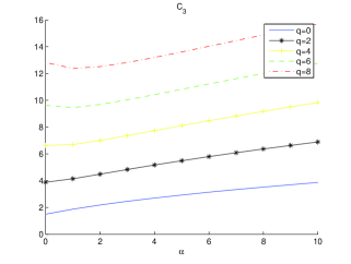
(a) $n=1$, $q=0,2,\cdots,8$ and $\alpha=0,1,\cdots,10$.

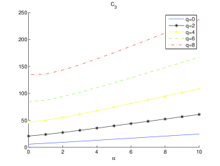
(b) $n=2$, $q=0,2,\cdots,8$ and $\alpha=0,1,\cdots,10$.

Figure 1: Values of $C_{3}$.

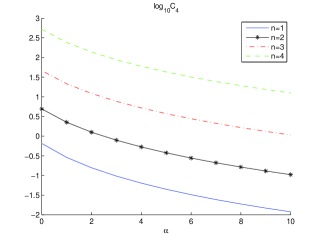
(a) $q=4$, $n=1,\cdots,4$ and $\alpha=0,1,\cdots,10$.

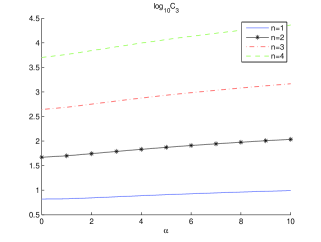
(b) $q=4$, $n=1,\cdots,4$ and $\alpha=0,1,\cdots,10$.

Figure 2: Values of $\log_{10}C_{4}$ and $\log_{10}{C}_{3}$.

3 Numerical tests

In order to demonstrate the efficiency and the stability of the previously proposed estimators, we present some numerical results in this section. First of all, we analyze the choice of parameters for these estimators.

3.1 Analysis for parameters’ choice for the bias term error and the noise error

As is shown previously, the proposed estimators contain two sources of errors: the bias term error which is produced by the truncation of the Jacobi orthogonal series expansion and the noise error contribution. The error bounds for these errors are given in Corollary 2.14. We are going to use the knowledge of the parameters’ influence to these error bounds. This will help us to obtain a tendency on the influence of these parameters on the estimation errors.

According to Corollary 2.13, we set $\alpha=\beta$ and choose the truncation order $q$ to be an even integer. On the one hand, it is clear that we should set $q$ as large as possible so as to improve the convergence rate and reduce the bias term error. On the other hand, the noise error contribution is bounded in Corollary 2.14 by $B_{noise}=C_{3}\frac{\delta}{h^{n}}$ where $C_{3}=\int_{-1}^{1}|Q_{\alpha,n,q}(t)|\,dt$. We can see in Figure 1 the different values of $C_{3}$ where $n=1,2$, $q=0,2,\cdots,8$ and $\alpha=0,1,\cdots,10$. It is clear that with the same values for $n$ and $\alpha$, $C_{3}$ increases with respect to $q$. Furthermore, it is easy to verify that $C_{3}$ increases with respect to $q$, independently of $n$ and $\alpha$. Hence, in order to reduce the bias term error and to avoid a large noise error, we set $q=4$ in our estimators. With this value, according to Corollary 2.14 the convergence rate is $O(\delta^{\frac{6}{n+6}})$.

The bias term error is bounded by $B_{bias}=\hat{C}_{2}h^{q+2}$ in Corollary 2.14 where $\hat{C}_{2}=\frac{{M}_{n+2+q}}{(n+q+2)!}\int_{-1}^{1}|t^{n+q+2}Q_{\alpha,n,q}(t)|\,dt$. Let us introduce $C_{4}=\int_{-1}^{1}|t^{n+q+2}Q_{\alpha,n,q}(t)|\,dt$. We can see in Figure 2 the different values of $\log_{10}C_{4}$ and $\log_{10}C_{3}$ when $n=1,\cdots,4$, $q=4$ and $\alpha=0,1,\cdots,10$. It is clear that $C_{4}$ decreases with respect to $\alpha$ while ${C}_{3}$ increases with respect to $\alpha$. Thus, in order to reduce the bias term error, we should set $\alpha$ as large as possible. However, a large value of $\alpha$ may produce a large noise error contribution. Here, we choose $\alpha=5$.

Until here, we have chosen $q=4$ and $\alpha=5$. The noise error decreases with respect to $h$ and the bias term error increases with respect to $h$. In the next subsection we are going to choose an appropriate value for $h$ by using the knowledge of function $f$ and by taking into account the numerical integration method error.

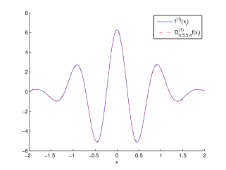
(a) $n=1$, $\alpha=5$, $q=4$ and $h=591T_{s}$.

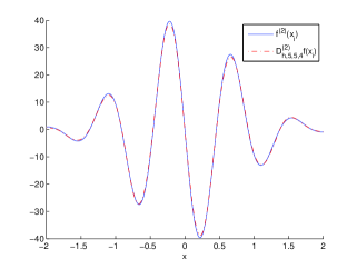
(b) $n=2$, $\alpha=5$, $q=4$ and $h=698T_{s}$.

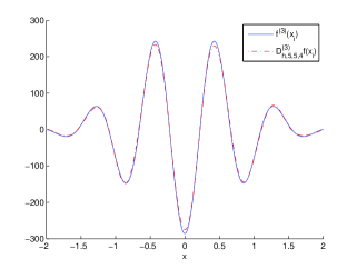
(c) $n=3$, $\alpha=5$, $q=4$ and $h=777T_{s}$.

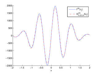
(d) $n=4$, $\alpha=5$, $q=4$ and $h=850T_{s}$.

Figure 3: The exact values of $f^{(n)}_{1}(x_{i})$ and the estimated values $D_{h,\alpha,\alpha,q}^{(n)}f_{1}(x_{i})$ for $\delta=0.15$.

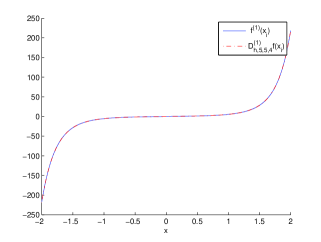
(a) $n=1$, $\alpha=5$, $q=4$ and $h=442T_{s}$.

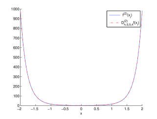
(b) $n=2$, $\alpha=5$, $q=4$ and $h=549T_{s}$.

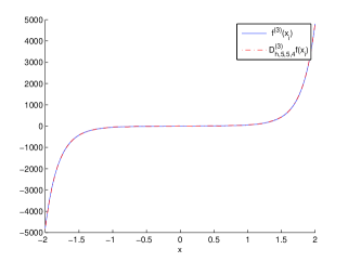
(c) $n=3$, $\alpha=5$, $q=4$ and $h=643T_{s}$.

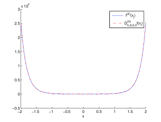
(d) $n=4$, $\alpha=5$, $q=4$ and $h=733T_{s}$.

Figure 4: The exact values of $f^{(n)}_{2}(x_{i})$ and the estimated values $D_{h,\alpha,\alpha,q}^{(n)}f_{2}(x_{i})$ for $\delta=0.15$.

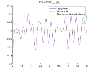
(a) $n=1$, $\alpha=5$, $q=4$ and $h=442T_{s}$.

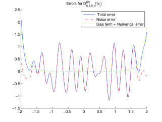
(b) $n=2$, $\alpha=5$, $q=4$ and $h=549T_{s}$.

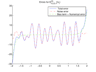
(c) $n=3$, $\alpha=5$, $q=4$ and $h=643T_{s}$.

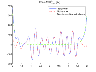
(d) $n=4$, $\alpha=5$, $q=4$ and $h=733T_{s}$.

Figure 5: The estimation errors for the estimated values $D_{h,\alpha,\alpha,q}^{(n)}f_{2}(x_{i})$ for $\delta=0.15$.

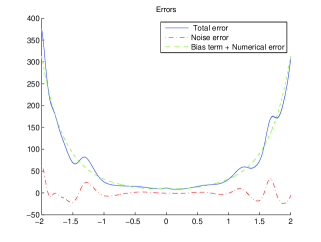
(a) The estimation errors for $D_{h_{i},5,5,4}^{(n)}f_{2}(x_{i})$ with varying values of $h_{i}$ for $\delta=0.15$.

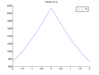
(b) Values of $m_{i}$

Figure 6: Errors for improved estimations with varying values of $h_{i}$.

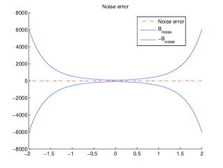
(a) Noise error with its error bounds

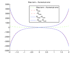
(b) Bias term error + numerical integration error with the error bounds

Figure 7: The estimation errors and their corresponding error bounds for $D_{h_{i},5,5,4}^{(n)}f_{2}(x_{i})$ with varying values of $h_{i}$ for $\delta=0.15$.

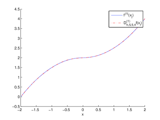
(a) $\delta=0.15$, $n=1$, $\alpha=5$, $q=4$ and $h=1700T_{s}$.

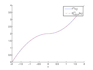
(b) $\delta=0.015$, $n=1$, $\alpha=5$, $q=4$ and $h=1200T_{s}$.

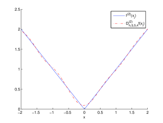
(c) $\delta=0.15$, $n=2$, $\alpha=5$, $q=4$ and $h=1700T_{s}$.

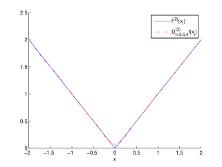
(d) $\delta=0.015$, $n=2$, $\alpha=5$, $q=4$ and $h=1200T_{s}$.

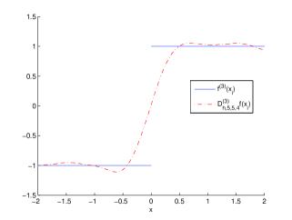
(e) $\delta=0.15$, $n=3$, $\alpha=2$, $q=2$ and $h=1700T_{s}$.

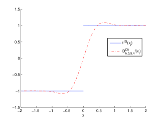
(f) $\delta=0.015$, $n=3$, $\alpha=2$, $q=2$ and $h=1500T_{s}$.

Figure 8: The exact values of $f_{3}^{(n)}(x_{i})$ and the estimated values $D_{h,\alpha,\alpha,q}^{(n)}f_{3}(x_{i})$.

3.2 Simulation results

The tests are performed by using Matlab R2007b. Let $f^{\delta}(x_{i})=f(x_{i})+c\varpi(x_{i})$ be a generated noise data with an equidistant sampling period $T_{s}=10^{-3}$ where $c>0$. The noise $c\varpi(x_{i})$ are simulated from a zero-mean white Gaussian $iid$ sequence by the Matlab function ’randn’ with STATE reset to $0$. By using the well-known three-sigma rule, we can assume that the noise level for $c\varpi$ is equal to $3c$. We use the trapezoidal method to approximate the integrals in our estimators with $2m+1$ values. The estimated derivatives of $f$ at the point $x_{i}\in I=[-2,2]$ are calculated from the noise data $f^{\delta}(x_{j})$ with $x_{j}\in[-x_{i}-h,x_{i}+h]$, where $h=mT_{s}$ and $2m+1$ is the number of sampling data used to calculate our estimation inside the sliding integration windows. When all the parameters are chosen, $Q_{\alpha,\beta,n,q}$ in the integrals of our estimators can be calculated explicitly by off-line work with the $O(n^{2})$ complexity. Hence, our estimators can be written like a discrete convolution product of these pre-calculated coefficients. Thus, we only need $2m+1$ multiplications and $2m$ additions to calculate each estimation.

The numerical integration method has an approximation error. Thus, the total error for our estimators can be bounded by

$$\begin{split}\left|T_{m}\left(Q_{\alpha,n,q}(\cdot)\,f^{\delta}(x_{i}+h\cdot)\right)-f^{(n)}(x_{i})\right|&\leq\left|T_{m}\left(Q_{\alpha,n,q}(\cdot)\,f^{\delta}(x_{i}+h\cdot)\right)-T_{m}\left(Q_{\alpha,n,q}(\cdot)\,f(x_{i}+h\cdot)\right)\right|\\ &+\left|T_{m}\left(Q_{\alpha,n,q}(\cdot)\,f(x_{i}+h\cdot)\right)-D_{h,\alpha,\alpha,{q}}^{(n)}f(x_{i})\right|+\left|D_{h,\alpha,\alpha,{q}}^{(n)}f(x_{i})-f^{(n)}(x_{i})\right|\\ &\leq B_{noise}+B_{num}+B_{bias}=B_{total},\end{split}$$

where $T_{m}\left(Q_{\alpha,n,q}(\cdot)\,f(x_{i}+h\cdot)\right)$ (resp. $T_{m}\left(Q_{\alpha,n,q}(\cdot)\,f^{\delta}(x_{i}+h\cdot)\right)$) is the numerical approximation to $D_{h,\alpha,\alpha,{q}}^{(n)}f(x_{i})$ (resp. $D_{h,\alpha,\alpha,{q}}^{(n)}f^{\delta}(x_{i})$) with the trapezoidal method and $B_{num}$ is the well-known error bound for the numerical integration error [36]:

$$\left|D_{h,\alpha,\alpha,{q}}^{(n)}f(x_{i})-T_{m}\left(Q_{\alpha,n,q}(\cdot)\,f(x_{i}+h\cdot)\right)\right|\leq\frac{2^{3}}{12(2m)^{2}}\sup_{t\in[-1,1]}\left(Q_{\alpha,n,q}(t)\,f(x_{i}+ht)\right)^{(2)}=B_{num}.$$ (58)

We are going to set the value of $m$ such that $B_{total}$ reaches its minimum and consequently the total errors in the following two examples can be minimized. For this, we need to calculate some values of $f^{(k)}$ with $k=0,\cdots,n+q+2$. According to Remark 4, we calculate the value of $M_{n+2+q}$ in the interval $[-2-\frac{h}{n+q+3},2+\frac{h}{n+q+3}]$. However, in practice, the function $f$ is unknown.

Example 1. We choose $f_{1}(x)=\sin(2\pi x)e^{-x^{2}}$ as the exact function. The numerical results are shown in Figure 3, where the noise level $\delta$ is equal to $0.15$. The solid lines represent the exact derivative values of $f_{1}^{(n)}$ for $n=1,2,3,4$ and the dash-dotted lines represent the estimated derivative values $D_{h,\alpha,\alpha,q}^{(n)}f_{1}(x_{i})$. Moreover, we give in Table 1 the total error values $\displaystyle\max_{x_{i}\in[2,2]}\left|D_{h,\alpha,\alpha,q}^{(n)}f_{1}(x_{i})-f^{(n)}_{1}(x_{i})\right|$ for the following noise levels: $\delta=0.15$ and $\delta=0.015$. We can see also the total error values produced with a larger sampling period $T^{\prime}_{s}=10T_{s}=10^{-2}$.

Table 1: $\displaystyle\max_{x_{i}\in[2,2]}\left|D_{h,5,5,4}^{(n)}f_{1}(x_{i})-f_{1}^{(n)}(x_{i})\right|$.

$\delta$	$n=1\ (m)$	$n=2\ (m)$	$n=3\ (m)$	$n=4\ (m)$
$0.15$	$9.45e-002\ (591)$	$1.1\ (698)$	$1.258e+001\ (777)$	$1.278e+002\ (850)$
$0.015$	$1.85e-002\ (425)$	$2.951e-001\ (523)$	$3.888\ (601)$	$4.588e+001\ (675)$
$0.015\,(T^{\prime}_{s}=0.01)$	$4.06e-002\ (47)$	$5.645e-001\ (55)$	$7.359\ (62)$	$9.686e+001\ (69)$

Example 2. When $f_{2}(x)=e^{x^{2}}$, we give our numerical results in Figure 4 with the noise level $\delta=0.15$, where the corresponding errors are given in Figure 5. In Table 2, we also give the total error values $\displaystyle\max_{x_{i}\in[2,2]}\left|D_{h,\alpha,\alpha,q}^{(n)}f_{2}(x_{i})-f_{2}^{(n)}(x_{i})\right|$ for $\delta=0.15$ and $\delta=0.015$, where the total error values are produced with $T_{s}$ and a larger sampling period $T^{\prime}_{s}=10^{-2}$.

Table 2: $\displaystyle\max_{x_{i}\in[2,2]}\left|D_{h,5,5,4}^{(n)}f_{2}(x_{i})-f_{2}^{(n)}(x_{i})\right|$.

$\delta$	$n=1\ (m)$	$n=2\ (m)$	$n=3\ (m)$	$n=4\ (m)$
$0.15$	$1.42e-001\ (442)$	$2.152\ (549)$	$2.982e+001\ (643)$	$3.756e+002\ (733)$
$0.015$	$2.22e-002\ (346)$	$4.435e-001\ (428)$	$5.973\ (510)$	$8.769e+001\ (595)$
$0.015\,(T^{\prime}_{s}=0.01)$	$3.404e-001\ (54)$	$3.425\ (61)$	$3.638e+001\ (68)$	$5.235e+002\ (79)$

We can see in Figure 5 that the maximum of the total error for each estimation (solid line) is produced nearby the extremities where the bias term error plus the numerical error (dash line) are much larger than the noise error. The noise error (dash-dotted line) is much larger elsewhere. This is due to the fact that the total error bound $B_{total}$ is calculated globally in the interval $[-h-2,2+h]$. The value of $m$ with which $B_{total}$ reaches its minimum is used for all the estimations $D_{h,\alpha,\alpha,q}^{(n)}f_{2}(x_{i})$ with $x_{i}\in[-2,2]$. This value is only appropriate for the estimations nearby the extremities, but not for the others. In fact, when the bias term error and the numerical integration error decrease, we should increase the value of $m$ so as to reduce the noise errors. In order to improve our estimations, we can choose locally the value of $m=m_{i}$, $i.e.$ we search the value $m_{i}$ which minimizes $B_{total}$ on $[-h_{i}+x_{i},x_{i}+h_{i}]$ where $h_{i}=m_{i}T_{s}$. We can see in Figure 6 the errors for these improved estimations $D_{h_{i},5,5,4}^{(n)}f(x_{i})$. The different values of $m_{i}$ are also given in Figure 6. The corresponding error bounds are given in Figure 7. We can observe that the error bounds proposed in this paper are correct but not optimal. However, the parameters’ influence to these error bounds can help us to know the tendency of errors so as to choose parameters for our estimations. On the one hand, the chosen parameters may not be optimal, but as we have seen in our examples, they give good estimations. On the other hand, the optimal parameters $q_{op}$, $\alpha_{op}$ and $m_{op}$ with which the total error bound reaches its minimum may not give the best estimation. That is why we only use these error bounds to choose the value of $m$.

Example 3. Let us consider the following function

$$f_{3}(x)=\left\{\begin{array}[]{rl}-\displaystyle\frac{1}{6}x^{3}+2x,&\text{ if }x\leq 0,\\ \displaystyle\frac{1}{6}x^{3}+2x,&\text{ if }x>0,\end{array}\right.$$

which is $C^{2}$ on $I=[-2,2]$. The second derivative of $f_{3}$ is equal to $|x|$. Consequently, $f_{3}^{(3)}$ does not exist at $x=0$. If $n\geq 1$, then this function does not satisfy the condition $f\in C^{n+2+q}(I)$ of Corollary 2.14. The numerical results are shown in Figure 8, where the sampling period is $T_{s}=10^{-3}$ and the noise level $\delta$ is equal to $0.15$ and $0.015$ respectively. The solid lines represent the exact derivative values of $f_{3}^{(n)}$ for $n=1,2,3$ and the dash-dotted lines represent the estimated derivative values $D_{h,\alpha,\alpha,q}^{(n)}f_{3}(x_{i})$. For the estimations of $f^{(1)}$ and $f^{(2)}$, we set $\alpha=5$ and $q=4$. When we estimate $f^{(3)}$, the noise error increases. Hence, we need to decrease the values of $\alpha$ and $q$ to $\alpha=2$ and $q=2$. In Table 3, we give also the total error values $\displaystyle\max_{x_{i}\in[2,2]}\left|D_{h,\alpha,\alpha,q}^{(n)}f_{3}(x_{i})-f_{3}^{(n)}(x_{i})\right|$ for $n=1,2$ and $\delta=0.015,0.15$.

Table 3: $\displaystyle\max_{x_{i}\in[2,2]}\left|D_{h,5,5,4}^{(n)}f_{3}(x_{i})-f_{3}^{(n)}(x_{i})\right|$.

$\delta$	$n=1\ (m)$	$n=2\ (m)$
$0.15$	$9.7e-003\ (1700)$	$9.65e-002\ (1700)$
$0.015$	$4.7e-003\ (1200)$	$7.23e-002\ (1200)$

References

- [1] Y. Chitour, Time-varying high-gain observers for numerical differentiation, IEEE Trans. Automat. Control 47 (2002) 1565-1569.
- [2] S. Ibrir, Linear time-derivatives trackers, Automatica 40 (2004) 397-405.
- [3] A. Levant, Higher-order sliding modes, differentiation and output-feedback control, Internat. J. Control 76 (2003) 924-941.
- [4] C.K. Chen, J.H. Lee, Design of high-order digital differentiators using error criteria, IEEE Trans. Circuits Syst. II 42(4) (1995) 287-291.
- [5] C.M. Rader, L.B. Jackson, Approximating noncausal IIR digital filters having arbitrary poles, including new Hilbert transformer designs, via forward/backward block recursion, IEEE Trans. Circuits Syst. I 53(12) (2006) 2779-2787.
- [6] J. Cheng, Y.C. Hon, Y.B. Wang, A numerical method for the discontinuous solutions of Abel integral equations, in: Inverse Problems and Spectral Theory, vol. 348, Contemp. Math. Amer. Math. Soc., Providence RI, 2004, pp. 233-243.
- [7] R. Gorenflo, S. Vessella, Abel integral equations: Analysis and applications, in: Lecture Notes in Mathematics, vol. 1461, Springer-Verlag, Berlin, 1991.
- [8] M. Hanke, O. Scherzer, Error analysis of an equation error method for the identification of of the diffusion coefficient in a quasi-linear parabolic differentical equation, SIAM J. Appl. Math. 59 (1999) 1012-1027. (electronic).
- [9] Z. Wang, J. Liu, Identification of the pollution source from one-dimensional parabolic equation models, Appl. Math. Comput. (2008) doi:10.1016/j.amc.2008.03.014.
- [10] I.R. Khan, R. Ohba, New finite difference formulas for numerical differentiation, J. Comput. Appl. Math. 126 (2000) 269-276.
- [11] R. Qu, A new approach to numerical differentiation and integration, Math. Comput. 24 (10) (1996) 55-68.
- [12] A.G. Ramm, A.B. Smirnova, On stable numerical differentiation, Math. Comput. 70 (2001) 1131-1153.
- [13] D.N. Hào, A. Schneider, H.J. Reinhardt, Regularization of a non-characteristic Cauchy problem for a parabolic equation, Inverse Probl. 11 (1995) 1247-1264.
- [14] D.A. Murio, The Mollification Method and the Numerical Solution of Ill-Posed Problems, John Wiley & Sons Inc., New York, 1993.
- [15] D.A. Murio, C.E. Mejía, S. Zhan, Discrete mollification and automatic numerical differentiation, Comput. Math. Appl. 35 (1998) 1-16.
- [16] G. Nakamura, S. Wang, Y. Wang, Numerical differentiation for the second order derivatives of functions of two variables, J. Comput. Appl. Math. 212 (2008) 341-358.
- [17] T. Wei, Y.C. Hon, Y. Wang, Reconstruction of numerical derivatives from scattered noisy data, Inverse Probl. 21 (2005) 657-672.
- [18] Y. Wang, X. Jia, J. Cheng, A numerical differentiation method and its application to reconstruction of discontinuity, Inverse Probl. 18 (2002) 1461-1476.
- [19] M. Mboup, C. Join, M. Fliess, Numerical differentiation with annihilators in noisy environment, Numer. Algorithms 50, 4 (2009) 439-467.
- [20] M. Mboup, C. Join, M. Fliess, A revised look at numerical differentiation with an application to nonlinear feedback control, in: 15th Mediterranean Conference on Control and Automation, MED’07, Athenes, Greece 2007.
- [21] C. Lanczos, Applied Analysis, Prentice-Hall, Englewood Cliffs, NJ, 1956.
- [22] S.K. Rangarajana, S.P. Purushothaman, Lanczos’ generalized derivative for higher orders, J. Comput. Appl. Math. 177 (2005) 461-465.
- [23] Z. Wang, R. Wen, Numerical differentiation for high orders by an integration method, J. Comput. Appl. Math. 234 (2010) 941-948.
- Fliess et al. [2004] M. Fliess, C. Join, M. Mboup, and H. Sira-Ramírez, Compression différentielle de transitoires bruités, C.R. Acad. Sci. I 339 (2004) 821-826. Paris.
- [25] M. Fliess, Analyse non standard du bruit, C.R. Acad. Sci. Paris Ser. I, 342 (2006) 797-802.
- Fliess and Sira-Ramírez [2003] M. Fliess and H. Sira-Ramírez, An algebraic framework for linear identification, ESAIM Control Optim. Calc. Variat., 9 (2003) 151-168.
- [27] M. Fliess, M. Mboup, H. Mounier, H. Sira-Ramírez, Questioning some paradigms of signal processing via concrete examples, in: H. Sira-Ramírez, G. Silva-Navarro (Eds.), Algebraic Methods in Flatness, Signal Processing and State Estimation, Editiorial Lagares, México, 2003, pp. 1-21.
- [28] M. Mboup, Parameter estimation for signals described by differential equations, Appl. Anal. 88 (2009) 29-52.
- [29] D.Y. Liu, O. Gibaru, W. Perruquetti, M. Fliess, M. Mboup, An error analysis in the algebraic estimation of a noisy sinusoidal signal, in: 16th Mediterranean Conference on Control and Automation, MED’08, Ajaccio, 2008.
- [30] M. Fliess, Critique du rapport signal à bruit en communications numériques - Questioning the signal to noise ratio in digital communications, in: International Conference in Honor of Claude Lobry, ARIMA (Revue africaine d’informatique et de Mathématiques appliquées), vol. 9, 2008, pp. 419-429, (available at http://hal.inria.fr/inria-00311719/en/).
- [31] G. Szegö, Orthogonal polynomials, 3rd edn. AMS, Providence, RI 1967.
- [32] N. Aronszajn, Theory of reproducing kernels. Trans. AMS 68(3), (1950) 337-404.
- [33] S. Saitoh, Theory of reproducing kernels and its applications, in: Pitman Research Notes in Mathematics, Longman Scientic Technical, UK 1988.
- [34] E.I. Poffald, The Remainder in Taylor’s Formula, Amer. Math. Monthly, 97 (3) (1990), 205-213.
- [35] Vladimir A. Zorich, Mathematical Analysis I, Springer-Verlag, Berlin, 2004, 219-232.
- [36] A. Ralston, A first course in numerical analysis, McGraw-Hill, New York, 1965.