Domain Wall Solutions of Spinor Bose-Einstein Condensates in an Optical Lattice

Abstract

We studied the static and dynamic domain wall solutions of spinor Bose-Einstein condensates trapped in an optical lattice. The single and double domain wall solutions are constructed analytically. Our results show that the magnetic field and light-induced dipolar interactions play an important role for both the formation of different domain walls and the adjusting of domain wall width and velocity. Moreover, these interactions can drive the motion of domain wall of Bose ferromagnet systems similar to that driven by the external magnetic field or the spin-polarized current in fermion ferromagnet.

During the past several decades, the dynamics of spatial domain wall have attracted more attention in ferromagnetism Mohn ; Volkov . The conventional ferromagnet is usually composed of fermions which contribute the main site-to-site exchange interaction owing to the direct Coulomb interaction among electrons and Pauli exclusion principle. This exchange interaction causes spin wave unstable, and its developing instability brings about the appearance of spatial domain walls or magnetic soliton Kose . The contribution of the magnetic dipole-dipole interaction to domain wall formation is usually neglected in practice because it is typically several orders of magnitude weaker than the exchange coupling in fermion ferromagnet.

However, the description of magnetism composed of Bosons are not well explored. Fortunately, a typical Bose system was realized in cold spinor ⁸⁷Rb gases Stenger ; Anderson and ²³Na gases Stamper which provided a totally new environment to understand magnetism comprehensively. The ferromagnetic spinor Bose gases have attracted numerous theoretical and experimental interests Ho ; Miesner ; Pu ; Zhang ; Strecker ; Kasa ; Sarlo ; Wxz ; Sadler ; Gu , and some general properties as in conventional fermion ferromagnets have been observed, such as spontaneous symmetry-broken ground state Ho , spin domains and textures Miesner , and normal spin-wave excitations spectrum Pu . Especially, the spontaneous symmetry breaking in ⁸⁷Rb spinor condensates Sadler clearly shows ferromagnetic domains and domain walls in a Bose ferromagnet. Recently, the ferromagnetism in a Fermi gas is also of interest fermi in the field of ultracold atoms.

Spinor Bose-Einstein condensates (BECs) trapped in an optical potential have internal degrees of freedom due to the hyperfine spin of the atoms which liberate a rich variety of phenomena. When the potential valley is so deep that the individual sites are mutually independent, spinor BECs at each lattice site behave like spin magnets and can interact with each other through both the magnetic and the light-induced dipole-dipole interactions which are no longer negligible due to the large number of atoms at each lattice site. These site-to-site dipolar interactions can cause the ferromagnetic phase transition Pu leading to a “macroscopic” magnetization of the condensate array and the spin-wave like excitation Pu ; Zhang and magnetic soliton lizd ; Lu analogous to the ferromagnetism in solid-state physics, but occur with bosons instead of fermions. Also, spinor BECs in an optical lattice is a typical physical realization of Salerno model Saler .

In this paper, we explore the domain wall solutions of spinor BECs trapped in an optical lattice and the roles of the magnetic and light-induced dipole-dipole interactions for the type of domain wall solutions and domain wall width and velocity.

We consider $F=1$ spinor condensates trapped in a one-dimensional optical lattice formed by two-polarized laser beams counter propagating along the $y$-axis and the two laser beams are detuned far from atomic resonance. Under the tight-binding approximation, the Hamiltonian takes the form Ho ; Miesner ; Pu ; Zhang

$$\hat{H} = \sum_{n}[\lambda_{a}^{\prime}\mathbf{\hat{S}}_{n}^{2}-\gamma_{B}\hat{S}_{n}\cdot\mathbf{B}-\sum_{l\neq n}J_{nl}^{\text{iso}}\mathbf{\hat{S}}_{n}\cdot\mathbf{\hat{S}}_{l}$$ (1)

$$-\sum_{l\neq n}J_{nl}^{\text{tran}}\left(\hat{S}_{n}^{+}\hat{S}_{l}^{-}+\hat{S}_{n}^{-}\hat{S}_{l}^{+}\right)],$$

where $\mathbf{\hat{S}}_{n}$ is the $n$th collective spin operator, defined as $\mathbf{\hat{S}}_{n}=\hat{a}_{\alpha}^{{\dagger}}(n)\mathbf{F}_{\alpha\upsilon}\hat{a}_{\upsilon}(n)$, with $\hat{a}$ being annihilation operator and $\mathbf{F}$ being the vector operator for the hyperfine spin of an atom. The first term in the Hamiltonian results from the spin-dependent interatomic collisions at a given lattice site, with $\lambda_{a}^{\prime}=(1/2)\lambda_{a}\int d^{3}r\left|\phi_{n}(\mathbf{r})\right|^{4}$, where $\lambda_{a}$ is proportional to the difference between the s-wave scattering lengths in the triplet and singlet channels Ho , and $\phi_{n}(\mathbf{r})$ is the ground-state wave function for $n$th site. The direction of the magnetic field $\mathbf{B}$ is along $z$-axis and $\gamma_{B}=\mu_{B}g_{F}$ is the gyromagnetic ratio, with $\mu_{B}$ being the Bohr magneton and $g_{F}$ the Landé factor. The last two terms describe the site-to-site spin coupling induced by both the static magnetic and the light-induced dipole-dipole interactions Zhang , with the form $J_{nl}^{\text{iso}}=J_{nl}^{\prime}+J_{nl}^{\prime\prime}$, where $J_{nl}^{\prime}=\mu_{0}\gamma_{B}^{2}/(16\pi\hbar^{2})\mathop{\textstyle\iint}d\mathbf{r}d\mathbf{r}^{\prime}\left|\phi_{n}(\mathbf{r})\right|^{2}\left|\phi_{l}(\mathbf{r-r}^{\prime})\right|^{2}/\left|\mathbf{r}^{\prime}\right|^{3}$, $J_{nl}^{\prime\prime}=-3\mu_{0}\gamma_{B}^{2}/(16\pi\hbar^{2})\mathop{\textstyle\iint}d\mathbf{r}d\mathbf{r}^{\prime}\left|\phi_{n}(\mathbf{r})\right|^{2}\left|\phi_{l}(\mathbf{r-r}^{\prime})\right|^{2}y^{\prime 2}/\left|\mathbf{r}^{\prime}\right|^{5}$, $J_{nl}^{\text{tran}}=\gamma U_{0}/(24\Delta\hbar^{2}k_{L}^{3})\mathop{\textstyle\iint}d\mathbf{r}d\mathbf{r}^{\prime}f_{c}\left(\mathbf{r}^{\prime}\right)e^{(-r_{\bot}^{2}-\left|\mathbf{r}_{\bot}-\mathbf{r}_{\bot}^{\prime}\right|^{2})/W_{L}^{2}}$ $\cos\left(k_{L}y-k_{L}y^{\prime}\right)\cos(k_{L}y)\mathbf{e}_{+1}\cdot\mathbf{W}(\mathbf{r}^{\prime})\cdot\mathbf{e}_{-1}\left|\phi_{l}(\mathbf{r-r}^{\prime})\right|^{2}$ $\left|\phi_{n}(\mathbf{r})\right|^{2}+3J_{nl}^{\prime\prime}/2$. Here the cutoff function $f_{c}\left(\mathbf{r}\right)=e^{-r^{2}/L_{c}^{2}}$ describes the effective interaction range of the light-induced dipole-dipole interaction, with $L_{c}$ being the coherence length associated with different decoherence mechanisms Java and $\Delta$ being the detuned frequency. The wave number $k_{L}=2\pi/\lambda_{L}$, the transverse coordinate $r_{\bot}=\sqrt{x^{2}+z^{2}}$, $W_{L}$ is the width of the lattice laser beams, and $U_{0}$ denotes the depth of optical lattice potential. The $\mathbf{e}_{\pm 1}$ are unit vectors in the spherical harmonic basis, and the form of tensor $\mathbf{W}\left(\mathbf{r}\right)$ can be found in Ref. Zhang . Eq. (1) shows that the static magnetic and the light-induced dipole-dipole interaction can lead to the isotropic spin coupling denoted by $J_{nl}^{\text{iso}}$ and anisotropic spin coupling in the transverse direction denoted by $J_{nl}^{\text{tran}}$.

From Hamiltonian (1) we can derive the Heisenberg equation of motion at $k$th site for the spin, i.e., $i\hbar\partial\hat{S}_{k}/\partial t=[\hat{S}_{k},\hat{H}]$. When the optical lattice is infinitely long and in the ultra-low temperatures for condensation, the operator can be treated as a classical vector, $\mathbf{\hat{S}}_{k}\rightarrow\mathbf{S}\left(y,t\right)$. Here we assume all nearest-neighbor interactions are same, which is a good approximation in one-dimensional optical lattice Konotop . Then we get the effective Landau-Lifshitz equation lizd

$$\frac{\partial}{\partial t}\mathbf{S}=\frac{1}{\hbar}\mathbf{S}\times[2Jd_{0}^{2}(\frac{\partial^{2}\mathbf{S}}{\partial y^{2}}\mathbf{-}\frac{4J^{\text{tran}}}{J}S^{z}\mathbf{e}_{z})+\gamma B\mathbf{e}_{z}],$$ (2)

where $J=2J^{\text{tran}}+J^{\text{iso}}$ and $d_{0}=\lambda_{L}/2$ being the lattice constant. In a rotating frame around $z$-axis with angular frequency $\gamma_{B}B/\hbar$ the spin vector $\mathbf{S}$ is related with the original one by the transformation $S_{+}\equiv S^{x}+iS^{y}=S_{+}^{\prime}e^{-i\gamma_{B}Bt/\hbar}$. Thus Eq. (2) becomes

$$\frac{\partial}{\partial t}\mathbf{S}=\mathbf{S}\times\left(\frac{\partial^{2}}{\partial y^{2}}\mathbf{S-}\beta S^{z}\mathbf{e}_{z}\right),$$ (3)

where the superscript (^′) is omitted for pithiness, and the time $t$ and coordinate $y$ is in unit $t_{0}=\hbar/\left(2J\right)$ and $d_{0}$, respectively. The parameter $\beta\equiv 4J^{\text{tran}}/J$ can be controlled by tuning the lattice laser beams and the shape of the condensate at each lattice site. Such a character makes the lattice atomic spin chain an ideal tool to study a diversity of spin-related phenomena.

Static domain wall solutions: We firstly seek for the single domain wall solution in the form

$$S^{x}=\frac{\cos\eta_{0}^{\prime\prime}}{\cosh\Theta_{0}},S^{y}=\frac{\sin\eta_{0}^{\prime\prime}}{\cosh\Theta_{0}},S^{z}=\tanh\Theta_{0},$$ (4)

where $\Theta_{0}=k_{0}y-\omega_{0}t+\eta_{0}^{\prime}$ with $\eta_{0}^{\prime}$, $\eta_{0}^{\prime\prime}$ being two real parameters, and $k_{0}$, $\omega_{0}$ to be determined. Substituting Eq. (4) into Eq. (3) we find that $\omega_{0}=0$ and $k_{0}=\sqrt{-\beta}$,

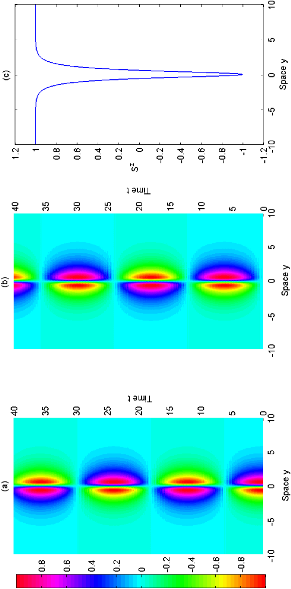
Figure 1: (Color online) The illustration of the double domain solutions (a) $S^{x}$, (b) $S^{y}$, and (c) $S^{z}$ in Eq. (5) with condition $\beta=-0.2$ and $k_{1}=0.3$. The two components $S^{x}$ and $S^{y}$ possess of the double peak located at $\sinh\Theta_{1}=\pm 1/\delta_{1}$.

and the solution (4) in fact denotes the static domain wall. This result implies the parameter $\beta<0$ which can be realized by a blue-detuned lattice $\left(\Delta<0\right)$, where the condensed atoms are trapped at the standing-wave nodes and the laser intensity is approximately zero. As a result, the light-induced dipole-dipole interactions is very small and the spin coupling is governed mainly by the static magnetic dipole-dipole interaction which implies $\left|\beta\right|<<1$. In this case the domain wall width, defined by $1/k_{0}$, can be adjusted mainly by $J^{\text{iso}}$. Under the condition $J^{\text{tran}}/J^{\text{iso}}\approx-0.25$, the domain wall width is about $\allowbreak 3d_{0}$ with $d_{0}$ being the lattice constant.

Eq. (3) has a norm form of Landau-Lifshitz type for a spin chain with an anisotropy. It can be solved by inverse scattering method where a couple of Lax equations is introduced for constructing the analytical solutions. In terms of our earlier results Licpl we get two static double domain wall solutions. The first has the form

$$S^{x} = -2\delta_{1}\left(\cos\Phi_{1}\sinh\Theta_{1}\right)/\Delta_{1},$$

$$S^{y} = -2\delta_{1}\left(\sin\Phi_{1}\sinh\Theta_{1}\right)/\Delta_{1},$$

$$S^{z} = 1-2/\Delta_{1},$$ (5)

where $\Delta_{1}=1+\delta_{1}^{2}\sinh^{2}\Theta_{1}$, $\Theta_{1}=[\beta/\left(8k_{1}\right)-2k_{1}]y$, $\Phi_{1}=[2k_{1}+\beta/\left(8k_{1}\right)]^{2}t$, $\delta_{1}=\left(16k_{1}^{2}+\beta\right)/\left(16k_{1}^{2}-\beta\right)$, and $k_{1}$ is a real parameter. The illustration of domain wall solution in Eq. (5) is shown in Fig. 1. From Fig. 1 and Eq. (5) we see that the two components $S^{x}$ and $S^{y}$ precess around the component $S^{z}$ with the frequency $\left(2k_{1}+\beta/\left(8k_{1}\right)\right)^{2}$, and the $z$-component of spin vector $S^{z}$ is conservative. The component $S^{x}$(or $S^{y}$) possess of the double peak located at $\sinh\Theta_{1}=\pm 1/\delta_{1}$ which varies with time periodically as shown in Fig. 1. The width of double domain wall is $1/\left(\beta/\left(8k_{1}\right)-2k_{1}\right)$, which is inverse proportion to the parameter $\beta$, while the maximum absolute value of valley for $S^{z}$ is constant.

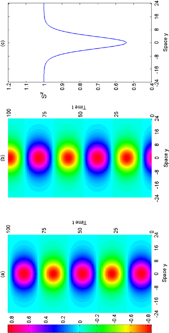
Figure 2: (Color online) The illustration of the double domain solutions (a) $S^{x}$, (b) $S^{y}$, and (c) $S^{z}$ in Eq. (6) with condition $\beta=-0.2$ and $\varphi=0.5$. The two components $S^{x}$ and $S^{y}$ possess of the single peak located at $z=0$.

The other solution can be written as

$$S^{x} = 2[\cot\varphi\sin\left(\varphi-\Phi_{2}\right)\cosh\Theta_{1}^{\prime}]/\Delta_{1}^{\prime},$$

$$S^{y} = 2[\cot\varphi\cos\left(\varphi-\Phi_{2}\right)\cosh\Theta_{1}^{\prime}]/\Delta_{1}^{\prime},$$

$$S^{z} = 1-2/\Delta_{1}^{\prime},$$ (6)

where $\Delta_{1}^{\prime}=1+\cot^{2}\varphi\cosh^{2}\Theta_{1}^{\prime}$, $\Phi_{2}=\beta\left(\cos^{2}\varphi\right)t$, $\Theta_{1}^{\prime}=-\sqrt{-\beta}\left(\sin\varphi\right)y$ , and $\varphi$ is a real parameter. The illustration of domain wall solution in Eq. (6) is shown in Fig. 2. Different from the former one, the two components $S^{x}$ and $S^{y}$ possess of the single peak located at $y=0$ which also oscillates with time periodically as shown in Fig. 2. The width of double domain wall is $1/(\sqrt{-\beta}\sin\varphi)$, which is inverse proportion to $\sqrt{-\beta}$. The maximum absolute value of valley for $S^{z}$ is $1-2/\left(1+\cot^{2}\varphi\right)$ which is also independent on the parameter $\beta$. We can rewrite $S^{z}$ in Eqs. (5) and (6) as $S^{z}=((\delta_{1}^{2}+1)\tanh^{2}\Theta_{1}-1)/((\delta_{1}^{2}-1)\tanh^{2}\left(-\Theta_{1}\right)-1)$ and $(\cot^{2}\varphi-1+\tanh^{2}\Theta_{1}^{\prime})/(\cot^{2}\varphi+1-\tanh^{2}\Theta_{1}^{\prime})$, respectively, which implies the double domain wall solutions can be written asymptotically as a nonlinear combination of two single domain wall solution in Eq. (4).

For observation of the above domain wall, one of the possible physical realizations of a gas of dipolar BECs can be provided by electrically polarized gases of polar molecules or by applying a high dc electric field to atoms Marinescu . In order to induce the dipole moment of the order $0.1$ D (Debye) one needs an electric field of the order of $10$ V/cm and the corresponding s-wave scattering length $10$-$1000$ Å.

Dynamic domain wall solutions: For red-detuned lattices, the condensed atoms are trapped at the maxima of the intensity of the standing wave laser and the spin coupling is dominantly determined by the light-induced dipole-dipole interaction. In particular, the spin coupling is anisotropic in this case. By controlling the laser parameters, we may always make the light-induced dipole-dipole interaction dominate over the static magnetic dipole-dipole interaction, i.e., $J^{\text{tran}}>>J^{\text{iso}}>0$ and $\beta\sim 2$.

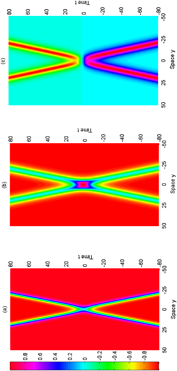
Figure 3: (Color online) The scattering process of two moving domain walls (a) $S^{x}$, (b) $S^{y}$, and (c) $S^{z}$ expressed in Eq. (8), in which two domain walls propagate with the opposite direction and the same absolute value of domain wall velocity in the condition $\beta=1.5$ and $\kappa=\pi/3$.

In this case we assume that the single moving domain wall solution of Eq. (3) admits the form

$$S^{x}=\tanh\Theta_{2},S^{y}=\frac{\cos\eta_{1}^{\prime\prime}}{\cosh\Theta_{2}},S^{z}=\frac{\sin\eta_{1}^{\prime\prime}}{\cosh\Theta_{2}},$$ (7)

where $\Theta_{2}=k_{2}y+\omega_{2}t+\eta_{1}^{\prime}$, with $\eta_{1}^{\prime}$, $\eta_{1}^{\prime\prime}$ being two real parameters, and $k_{2}$, $\omega_{2}$ to be determined. Substituting Eq. (7) into Eq. (3) we obtain $\omega_{2}=\beta/2\sin\left(2\eta_{1}^{\prime\prime}\right)$ and $k_{2}=\pm\sqrt{\beta}\sin\eta_{1}^{\prime\prime}$. The solution (7) shows that the dynamics of domain wall is restricted in ($k_{2},\omega_{2}$)-space, with $\left|k_{2}\right|_{\max}=\sqrt{\beta}$ and $\left|\omega_{2\max}\right|=\beta/2$. The width of domain wall, defined by $1/\left|k_{2}\right|$, is inverse proportion to the square root of parameter $\beta$ determined mainly by light-induced dipole-dipole interaction and the angle $\eta_{1}^{\prime\prime}$ of the three components of pseudospin vector $\mathbf{S}$. The domain wall velocity, i.e., $v=\omega_{2}/k_{2}=\pm\sqrt{\beta}\cos\eta_{1}^{\prime\prime}$, is dependent on the parameters $\beta$ and $\eta_{1}^{\prime\prime}$. When $\eta_{1}^{\prime\prime}=n\pi$, $n=0,1,2,...,$ the domain wall velocity attains its maximum value $v_{\max}=\sqrt{\beta}$. When $\eta_{1}^{\prime\prime}=\left(n+1/2\right)\pi,n=0,1,2,...$, the solution in Eq. (7) represents the static domain wall solution of Eq. (3) similar the case of $\beta<0$. It is interesting to estimate the velocity of domain wall. As a example, we consider the $F=1$ electronic ground state of ⁸⁷Rb which the Landé factor $g_{F}=-1/2$ and the gyromagnetic ratio $\gamma_{B}=-\mu_{B}/2$. As from Ref. Pu we estimate $J^{\text{iso}}$ is about $1.\allowbreak 1\times 10^{-36}$J with $\lambda_{L}=852$ nm. Asumming that $J^{\text{tran}}=10J^{\text{iso}}$ we have $\beta\approx 1.\allowbreak 9$ and the maximum domain wall velocity is about $v=$ $\sqrt{\beta}d_{0}/t_{0}\approx\allowbreak 130$ nm/s. For chromium atoms, it has a magnetic moment $6\mu_{B}$ and the corresponding domain wall velocity is about tens of domain wall velocity of ⁸⁷Rb with the same assumption.

The above results show that the domain wall velocity can be controlled by the parameter $\beta$ resulting from the external magnetic and light field-induced dipole-dipole interaction and the direction of pseudospin vector $\mathbf{S}$. In fermion ferromagnet, a magnetic domain wall is a spatially localized configuration of magnetization, in which the direction of magnetic moments gradually inverses. When a spin-polarized electric current flows through a domain wall, the spin-polarization of conduction electrons can transfer spin momentum to the local magnetization, thereby applying a spin-transfer torque, which manipulates the motion of domain wall Slon ; Katine similar to that driven by applied an external magnetic field Walker . It is interesting that our domain wall solution in Eq. (7) shows the same properties as that in fermion ferromagnet, i.e., for red-detuned lattices the light-induced dipolar interactions can be seen as the external force to drive the motion of domain wall, and it has the potential contribution for the research of domain wall motion in the Bose ferromagnet systems.

The dynamic double domain wall solution can be constructed by employing Hirota method Mic which is an effective straightforward technique to solve the nonlinear equations. Here we only mention the main idea of Hirota method briefly. Firstly, it applies a direct transformation to the nonlinear equation. Then, by means of some skillful bilinear operators the nonlinear equation can be decoupled into a series of equations. With some reasonable assumptions the exact solutions can be constructed effectively. Performing the normal procedure in Ref. Mic we get dynamic double domain wall solution as

$$S^{x} = [e^{\theta}\cosh^{2}\left(k_{2}^{\prime}y\right)-\sinh^{2}\left(\omega_{2}^{\prime}t\right)-\cos^{2}\kappa]/\Delta_{2},$$

$$S^{y} = 2e^{\theta/2}\cos\kappa\cosh\left(k_{2}^{\prime}y\right)\cosh\left(\omega_{2}^{\prime}t\right)/\Delta_{2},$$

$$S^{z} = -2e^{\theta/2}\sin\kappa\cosh\left(k_{2}^{\prime}y\right)\sinh\left(\omega_{2}^{\prime}t\right)/\Delta_{2},$$ (8)

where $\Delta_{2}=e^{\theta}\cosh^{2}\left(k_{2}^{\prime}y\right)+\sinh^{2}\left(\omega_{2}^{\prime}t\right)+\cos^{2}\kappa$ with the real parameter $\kappa$, $k_{2}^{\prime}=\pm\sqrt{\beta}\sin\kappa$, $\omega_{2}^{\prime}=\beta/2\sin\left(2\kappa\right)$, and $\theta=\ln\left(\cos^{2}\kappa\right)$. In figure 3 we plot the evolution of double domain wall solution $\mathbf{S}$ in Eq. (8). From figure 3 we see that the double domain solution in Eq. (8) presents a general scattering process of two moving domain walls which propagate with the opposite direction and the same absolute value of domain wall velocity $\sqrt{\beta}\cos\kappa$. Analysis reveals that there is no amplitude exchange among the components $S^{x}$ for two domain walls. However, there is a small shift for the center of each domain wall during collision.

In conclusion, we have presented two kinds of domain wall solutions of dipolar spinor BECs in an optical lattice based on an effective Hamiltonian of anisotropic pseudospin chain. In real experiment, the magnetic field and light-induced dipolar interactions are related with the detuned term which can be controlled easily by the external magnetic and light field. Our results show that we can control this site-to-site spin coupling of the condensates at each lattice to form the different domain wall solutions. Especially, since these magnetic field and light-induced dipolar interactions are highly controllable, the spinor BECs in an optical lattice as an exceedingly clean system offer a very useful tool to study spin dynamics in periodic structures and to understand ferromagnetism comprehensively.

Acknowledgements: This work was supported by NSF of China under Grants No. 10874038 and No. 10804028 and the NSF of

Hebei Province of China under Grant No. A2007000006. J.-Q. Liang was supported by NSF of China under Grant No. 10775091. W. M. Liu was supported by NSFC under Grants No. 60525417, No. 10740420252, and No. 10874235 and by NKBRSFC under Grants No. 2006CB921400 and No. 2009CB930704.

References

- (1) P. Mohn, Magnetism in the Solid state: An Introduction (Springer-Verlag, Berlin, 2003).
- (2) V. V. Volkov and V. A. Bokov, Physics of the Solid State, 50 199 (2008).
- (3) A. M. Kosevich, B.A. Ivanoy, A.S. Kovalev, Phys. Rep. 194, 117 (1990).
- (4) J. Stenger, et al., Nature (London) 396, 345(1998).
- (5) B. P. Anderson and M. A. Kasevich, Science 282, 1686 (1998).
- (6) D. M. Stamper-Kurn et al., Phys. Rev. Lett. 80, 2027 (1998); D. M. Stamper-Kurn et al., Phys. Rev. Lett. 83, 661 (1999).
- (7) H.-J. Miesner et al., Phys. Rev. Lett. 82, 2228 (1999).
- (8) T. L. Ho, Phys. Rev. Lett. 81, 742 (1998); C. K. Law et al., Phys. Rev. Lett. 81, 5257 (1998); T. Ohmi and K. Machida, J. Phys. Soc. Jpn. 67, 1822 (1999).
- (9) H. Pu et al., Phys. Rev. Lett. 87, 140405 (2001); Kevin Gross et al., Phys. Rev. A. 66, 033603 (2002); H. J. Lewandowski et al., Phys. Rev. Lett. 88, 070403 (2002).
- (10) Weiping Zhang et al., Phys. Rev. Lett. 88, 060401 (2002).
- (11) Kevin E. Strecker et al., Nature (London) 417, 150 (2002); L. Salasnich et al., Phys. Rev. Lett. 91, 080405 (2003); L. D. Carr and J. Brand, Phys. Rev. Lett. 92, 040401 (2004).
- (12) K. Kasamatsu and M. Tsubota, Phys. Rev. Lett. 93, 100402 (2004).
- (13) L. De Sarlo et al., Phys. Rev. A 72, 013603 (2005); C. Tozzo et al., Phys. Rev. A 72, 023613 (2005).
- (14) Wenxian Zhang et al., Phys. Rev. Lett. 95, 180403 (2005).
- (15) L. E. Sadler et al., Nature (London) 443, 312 (2006).
- (16) Q. Gu et al., Phys. Rev. A 70, 063609 (2004); Qiang Gu and Haibo Qiu, Phys. Rev. Lett. 98, 200401 (2007).
- (17) L. J. LeBlanc, et al., Phys. Rev. A 80, 013607 (2009); S. Trotzky et al., Science 319, 295 (2008); Gyu-Boong Jo, et al., Science 325, 1521 (2009).
- (18) Zai-Dong Li et al., Phys. Rev. A 71, 053611 (2005); Lu Li et al., Phys. Rev. E 73, 066610 (2006); Zai-Dong Li, Q.-Y. Li, Ann. Phys. (N.Y.) 322, 1961 (2007); Z. W. Xie et al., Phys. Rev. A 69, 053609 (2004).
- (19) Lu Li et al., Phys. Rev. A 72, 033611 (2005); Lei Wu et al., Phys. Rev. A 78, 053807 (2008).
- (20) M. Salerno, Phys. Rev. A 46, 6856 (1992); J. Gomez-Gardeñs et al., Phys. Rev. E 73, 036608 (2006).
- (21) J. Javanainen, Phys. Rev. Lett. 72, 2375 (1994).
- (22) V. V. Konotop et al., Phys. Rev. E 56, 7240 (1997).
- (23) Zai-Dong Li et al., Chin. Phys. Lett. 20, 39 (2003).
- (24) M. Marinescu and L. You, Phys. Rev. Lett. 81, 4596 (1998).
- (25) N. L. Schryer et al., J. Appl. Phys. 45, 5406 (1974); J. C. Slonczewski, J. Magn. Magn. Mater. 159, L1 (1996); L. Berger, Phys. Rev. B 54, 9353 (1996).
- (26) Y. B. Bazaliy et al., Phys. Rev. B 57, R3213 (1998); J. A. Katine et al., Phys. Rev. Lett. 84, 3149 (2000); G. Tatara et al., Phys. Rev. Lett. 92, 086601 (2004); Zai-Dong Li et al., Phys. Rev. E 76, 026605(2007). P. B. He, et al. Phys. Rev. B 72, 064410 (2005); P. B. He, et al. Phys. Rev. B 72, 172411 (2005).
- (27) A. A. Thiele, Phys. Rev. B 7, 391 (1973); N. L. Schryer, et al., J. Appl. Phys. 45, 5406 (1974).
- (28) Michael Svendsen et al., J Phys. A 26, 1717 (1993).