Generalized Lyapunov Exponent and Transmission Statistics in One-dimensional Gaussian Correlated Potentials
Abstract
Distribution of the transmission coefficient of a long system with a correlated Gaussian disorder is studied analytically and numerically in terms of the generalized Lyapunov exponent (LE) and the cumulants of . The effect of the disorder correlations on these quantities is considered in weak, moderate and strong disorder for different models of correlation. Scaling relations between the cumulants of are obtained. The cumulants are treated analytically within the semiclassical approximation in strong disorder, and numerically for an arbitrary strength of the disorder. A small correlation scale approximation is developed for calculation of the generalized LE in a general correlated disorder. An essential effect of the disorder correlations on the transmission statistics is found. In particular, obtained relations between the cumulants and between them and the generalized LE show that, beyond weak disorder, transmission fluctuations and deviation of their distribution from the log-normal form (in a long but finite system) are greatly enhanced due to the disorder correlations. Parametric dependence of these effects upon the correlation scale is presented.
pacs:
05.40.-a, 72.15.Rn, 42.25.Dd, 42.25.BsI Introduction
Properties of stochastic systems can be significantly affected by the degree of correlation of the external noise term (see, e.g., Ref. Hanggi-95 and references therein). As an example of such phenomenon, we study statistical properties of Anderson localization Anderson-58 in a linear one-dimensional model
| (1) |
with correlated disorder potential . With a suitable change of notation, equation (1) can describe a stationary problem either for a quantum particle at energy , or for classical scalar electromagnetic or acoustic waves. Equation (1) appears also in many other fields of physics. For example, with considered time, Eq. (1) represents a random frequency oscillator, which is a simple paradigm of a stochastic dynamical system (see Ref. Pikovsky-03 for a more detailed discussion of this and other applications). In all these instances, an important quantity is the Lyapunov exponent (LE) , where and is a solution of an initial value problem. LE is a non-random quantity independent of the specific realization of disorder LGP-Introduction . On the contrary, ”local” LE is random and should be described statistically by distribution . Distribution can be studied in terms of its cumulants (e.g. Ref. Schomerus-02 ) or using the generalized Lyapunov exponents , where denotes average over the disorder realizations (e.g., Refs. Pikovsky-03 ,Paladin-87 ).
LEs and are intimately related to the localization properties of one-dimensional disordered systems. The latter was studied extensively and it is rigorously established that almost all eigenstates in one-dimentional (1D) disordered systems are exponentially localized under rather general conditions Kotani-82 ,Simon-83 ,Kotani-87 (see also LGP-Introduction ,Pastuf-Figotin and references therein). The inverse localization length of the eigenstates, as well as the asymptotic decay rate of the transmission coefficient of the system of length , are equal LGP-Introduction to the LE . More generally, statistical properties of the quantity and of the introduced above local LE become asymptotically equivalent for large (see Sec. II). Therefore, in what follows, we discuss the problem in terms of the transmission coefficient , while the results apply in a broader context of the local LE .
Transmission coefficient is a basic characteristics of the wave transport through the non-uniform media. In the electronic systems, is related to the dimensionless conductance by the Landauer formula Landauer-70 . Measurement of the transmission coefficients is one of the ways to investigate different aspects of Anderson localization experimentally. Some indications of Anderson localization were observed with light Light-Loc , microwaves Micro-W-Loc , cold atoms Aspect-1DBECexper-08 and ultrasound Sound-Loc . In most of these experiments, the correlation scale of the randomness is comparable to the scattered wavelength and should be taken into account to obtain a full quantitative description. In the experiments in Ref. Aspect-1DBECexper-08 , localization of cold atoms was found by observing localized density profiles, rather than transmission. Recently, possible experiments on cold atom transmission through the disordered optical potentials were discussed Ernst-10 . It is worth noting that in the actively developing field of cold atoms, one of the ways to introduce disorder is by using the laser speckle intensity patterns, which are highly correlated Aspect-Speckle-06 . On the theoretical side, there is an increasing interest in the disordered systems with correlated potentials. In particular, in 1D systems, disorder correlations were found to have strong effect both on the localization length LGP-Introduction ,Israilev-99 ,Tessiery-Israilev-01 ,Gurevich ,Palencia-09 , on the generalized LE Tessieri-02 ,Iomin-09 and on the transmission statistics Titov-05 ,Deych-03 and, in special cases, even lead to the appearance of extended states Extend-Stats .
The main subject of the present work, is the effect of disorder correlations on the transmission statistics in the asymptotic limit of large . Transmission coefficient of a long disordered system exhibits large sample-to-sample fluctuations and is not a self-averaging quantity. General properties of the transmission distribution have been considered in the past using the composition rule for the transmission of a one-dimensional chain of statistically identical and independent (or only weakly dependent) random scatterers Anderson-80 ,Shapiro-88 . It was shown that a convenient variable to deal with is , since it can be represented as a sum of independent (or weakly dependent) random variables, for which the conditions of the Central Limit theorem, or its modification for weakly correlated variables, are valid. Then, by additivity of cumulants of independent variables, it follows that all cumulants of the -distribution, , grow at most linearly in the system length :
| (2) |
Here denotes th-order cumulant of the quantity , and the asymptotic cumulant coefficients are constants, which depend on the microscopic properties of the system. The above result applies to systems with both uncorrelated and correlated random potentials, provided the considered system can be divided into blocks, which are much longer than the disorder correlation scale and can be treated as nearly independent scatterers.
Thus, the general form of the large- limit of the transmission distribution is well understood, and the remaining questions are about the dependence of the cumulant coefficients on the parameters of the problem. According to Eq. (2), transmission statistics can be discussed at the following three levels of ”resolution”. First, there exists a self-averaging quantity , which has a non-random limit
| (3) |
At this level, all the information about the transmission fluctuations is lost in the asymptotic limit . Next, one can define a variable , where , for which the Central Limit theorem holds, and whose cumulants of the order vanish in the asymptotic limit as . Therefore, this veriable has a limiting Gaussian distribution with zero mean and unit variance. Limiting probability distributions and their relation to universality and scaling have been discussed in the past Shapiro-88 ,Shapiro-87 . In the present context of a 1D problem, only two model-dependent parameters, and , are ”remembered” in the limiting distribution of . This fact is referred to as ”two-parameter scaling” Shapiro-88 . In special conditions, namely when the combined scatterers are weak and their reflection phases are distributed uniformly, the composition rule yields up to weak disorder corrections, which is a manifestation of single parameter scaling (SPS) Anderson-80 ,Shapiro-88 .
Finally, for large but finite , one can study the non-Gaussian corrections to the limiting Gaussian distribution, which are characterized by the asymptotic cumulant coefficients , . The latter are responsible for the extreme fluctuations of the transmission coefficient. These large deviations can also be studied in terms of the generalized LEs, which describe asymptotic growth rates of the moments of the inverse transmission coefficient and can be expressed as a sum over ’s Pikovsky-03 .
Under conditions of weak scattering and phase randomization, in addition to the SPS relation , it was found in some models of disorder that cumulant ratios , , vanish up to the weak disorder corrections Schomerus-02 ,Petri-96-97 . Vanishing of higher cumulants is also indicated by the coincidence of LE and the second order generalized LE in the lowest order of the weak disorder expansion, which is valid for a wide variety of 1D disordered models Pikovsky-03 ,LGP-Introduction ,Tessiery-Israilev-01 ,Tessieri-02 . Thus, quite generally, cumulant coefficients satisfy
| (4) |
which holds up to the weak disorder corrections.
Considerable analytical and numerical effort was devoted to verification of SPS and determining limits of its validity for various models of disorder Schomerus-02 ,Shapiro-88 ,Petri-96-97 ,Abrikosov-81 ,Altshuler-01 ,Tamura-93 ,Zaslavsky-97 . Usually, SPS holds for sufficiently weak disorder, when the localization length is much larger than other scales in the problem (see also discussion in Ref. Altshuler-01 ).
Deviations from relations (4) were studied for uncorrelated disorder Pikovsky-03 ,Schomerus-02 ,Schomerus-03 as well as for some specific models of correlated disorder potentials Titov-05 ,Deych-03 . In particular, for the continuous white noise model, it was shown Schomerus-02 that for large positive energy (weak disorder), becomes slightly different from unity near and vanishes for large negative , while the ”non-Gaussian” ratios have numerical values of about a fraction of unity near , and vanish for large negative or positive (energy scale is determined by strength of disorder). Thus, in the white noise model, unless is sufficiently large and negative, the relative width of the Gaussian bulk of the -distribution depends weakly on the disorder strength, while finite higher cumulants indicate that some non-Gaussian corrections to the distribution tails develop in strong disorder. The latter was also observed in Ref. Pikovsky-03 , where distribution of local Lyapunov exponents was studied in terms of the generalized LEs for a continuous -correlated disorder.
Presence of disorder correlations can significantly enhance deviation from relations (4). For instance, one finds near certain energies of the tight-binding model with a weak short-range correlated disorder Titov-05 . Another example of the effect of correlations is scaling relation , obtained in Ref. Deych-03 for strong exponentially correlated dichotomous disorder with a correlation scale . This scaling, which replaces Eq. (4), is valid when , which means , so that Gaussian bulk of the distribution becomes much broader than in weak or white noise disorder.
These special examples suggest that disorder correlations can have a significant effect on the transmission statistics. One can distinguish two limiting regimes. In weak disorder, which can be treated perturbatively, LE depends strongly on the correlation scale LGP-Introduction ,Israilev-99 ,Gurevich ,Palencia-09 . However, it usually remains the only parameter of the transmission distribution, and relations (4) stay valid Petri-96-97 ,Tamura-93 ,Zaslavsky-97 . Another special regime, which can be called a semiclassical regime of strong disorder, occurs when typical random potential barriers are higher than energy and sufficiently broad, so that tunneling probability already through a single random barrier becomes small. In this case localization is dominated by the under-barrier tunneling, and one can generalize the semiclassical approach of Ref. Deych-03 to study the distribution of in terms of the statistics of disorder excursions above the level . In the present work we use this approximation for the strong disorder regime to show that .
The main focus of the present research is, however, on the effect of disorder correlations on the transmission distribution at the transition between these two limiting regimes. We consider model (1) with Gaussian disorder , whose correlation function is arbitrary, except for the assumption that it is parametrized with a finite correlation scale . The transmission statistics is studied in terms of the dimensionless ratios , and . Quantity characterizes extreme fluctuations of the inverse transmission coefficient , since it is related to the ratio of the average to the typical values of . In addition, it can be used to show violation of relations (4), because when these relations hold Pikovsky-03 ,Tessieri-02 .
To calculate , which can not be treated exactly in a general case of correlated disorder, we develop a small- approximation Klatzkin . A simple regularization is proposed to extend this method to the power law correlations, for which a standard approximation turns out to be inapplicable. Numerical simulations are used to verify the analytical approximation for and to calculate cumulant coefficients for different types of correlations and for different values of (and ). As expected, the obtained results for , and show that SPS and Eq. (4) hold in the weak disorder limit. Beyond this regime, we find that disorder correlations strongly enhance deviations from relations (4), as compared to the case of white noise, and lead to increase of both typical and extreme fluctuations of transmission. Dependence of these effects on the parameters and is discussed ( is the wavenumber). In general, effect of disorder correlations on the transmission statistics becomes important when , i.e. the ratio between the correlation and the localization lengths, is comparable to or greater than unity.
The outline of the paper is as follows. In Sec. II we define the model in question and discuss in some more detail the standard and the generalized Lyapunov exponents. The small- approximation for the generalized LE is developed in Sec. III. First, using the analogy of Eq. (1) with the Langevin equation, equations for the second moments of are obtained by means of the Furutsu-Novikov formula. This leads to an infinite hierarchy of the integro-differential equations for the second moment of the wave function and its functional derivatives Hanggi-95 ,Klatzkin . Then, the small- closure approximation is applied and the result is compared to numerical simulations. In Sec. IV we obtain scaling relations for in the semiclassical regime of strong disorder. In Sec. V analytical and numerical results for and are used to discuss properties of the asymptotic distribution of the transmission coefficient and deviation from relations (4). The results are summarized in Sec. VI. Known results on the generalized LE for the -correlated disorder and on the Born approximation are presented in appendices A and B respectively. Method of numerical simulation is explained in Appendix C. Some auxiliary formulae for the semiclassical treatment of strong disorder are presented in Appendix D.
II Basic equations
We consider one-dimensional Schrödinger equation
| (5) |
where is energy and is zero-mean Gaussian disorder potential. The latter is completely described by its two-point correlation function , written as
| (6) |
where and are disorder variance and correlation length, and the dimensionless function decays on the scale of unity and is chosen so that
| (7) |
The white noise model is obtained by taking the limit , while keeping constant:
| (8) |
where we have introduced disorder intensity parameter
| (9) |
The transmission properties of a one-dimensional system of finite length are described by transfer matrix Mello-Kumar
| (10) |
which relates amplitudes of the incident and the outgoing waves (a time reversal invariance is implied). Here and are reflection and transmission phases respectively. In the following sections, generalized LE and asymptotic cumulant coefficients are studied in terms of the amplitude , where is a solution of (5) satisfying some generic initial conditions, e.g. , . The obtained results are valid also for the transmission coefficient , since in the asymptotic limit it becomes statistically equivalent to the amplitude . This is because is expressed in terms of the transfer matrix (10), which asymptotically factorizes into the product of large factor and statistically independent of it matrix of the order of unity. Such factorization takes place, since for much larger than the localization length, phases and become statistically (almost Note-T-phase-Coorel ) independent of , while coefficient becomes exponentially small in most realizations of disorder. Thus, for large , one can write
| (11) |
where the term , which absorbs phases and the initial conditions for , is statistically independent of the first one, and its cumulants are of the order of unity. Therefore, using additivity of cumulants of independent variables, one has (cf. Eq.(2))
| (12) |
Thus, for large , inverse transmission coefficient is statistically equivalent to the amplitude , and, thus, to the local LE , defined in the introduction. In particular, LE coincides with , and in the following we will use the latter notation.
As already mentioned in the introduction, cumulant coefficients describe asymptotic form of the distribution . Introducing the dimensionless length measured in units of the localization length , cumulants of can be rewritten as (cf. Eq. (2))
| (13) |
Therefore, it is convenient to discuss transmission distributions in terms of the dimensionless ratios , since meaningful comparison of transmission fluctuations in different models of disorder should be done for the same dimensionless system length . Then, for instance, relative fluctuation of is expressed as .
Another quantity which characterizes transmission distribution is second order generalized LE defined by Paladin-87
| (14) |
Since is a cumulant generating function of the distribution , the generalized LE is related to all cumulant coefficients by the expression
| (15) |
For large , value of is dominated by the long tail of the -distribution, which becomes highly skewed and heavy-tailed. Therefore, rather than representing typical values of , generalized LE provides useful complementary information about the low- tail of its distribution. To this end, it is convenient to define the following quantity
| (16) |
whose meaning is twofold. On the one hand, deviation of the value of from unity gives an integral measure of deviation from the universal weak disorder relations (4), since when these relations hold (cf. Ref. Pikovsky-03 ). On the other hand, can be used to characterizes the extreme relative fluctuations of the inverse transmission coefficient in terms of the ratio between the mean and the typical values of :
| (17) |
III Generalized Lyapunov Exponent
III.1 Equation of motion for moments
The linearity of the Schrödinger equation (5) allows one to obtain closed-form equations for the -order products , where, . To this end, we rewrite Eq. (5) in the form of the Langevin equation. The coordinate is considered as a formal time on the half axis and the dynamical variables are introduced. In these variables the Langevin equation reads
| (18) |
where is now the correlated noise. We need to consider an initial value problem for the second order moments , , , whose asymptotic exponential growth rate gives the generalized LE , Eq. (14). Introducing vector
| (19) |
and using Eq. (18), one obtains
| (20) |
where
| (21) |
and is an initial condition. To obtain equation for , Eq. (20) is averaged over the disorder, which introduces correlator :
| (22) |
Applying the Furutsu-Novikov formula Hanggi-95 ,Klatzkin yields
| (23) |
where is a functional derivative of with respect to and is the disorder correlation function (6). Since equation (23) contains a new quantity , it is not closed with respect to . An important exception is the case of the uncorrelated disorder, which is considered in Appendix A, and will be used in the forthcoming analysis. In general case, to proceed further, an additional equation for is required, which is obtained by differentiating Eq. (20) functionally with respect to , and using the differentiation property Klatzkin . This yields
| (24) |
where is the Heaviside step function. For , Eq. (24) can be rewritten as
| (25) |
The causality property was used in derivation of Eq. (24). It follows from the fact that obeys first order differential equation (20) with an initial condition at and, thus, is independent of at the time later than . Then, integration of the differential equation (24) over from some up to yields the initial condition in Eq. (25).
Note that functional derivative in Eq. (25) and vector in Eq. (20) obey the same differential equation, but with different initial condition. Due to this similarity, moments and grow with the same asymptotic rate for large and respectively. The difference between the two quantities is that the initial condition for depends on and, therefore, it is correlated to .
Averaging Eq. (25) over the disorder and using the Furutsu-Novikov formula, one obtains the following equation for the moment :
| (26) |
with the initial condition
| (27) |
Thus, Eq. (26) is again not closed with respect to , because it contains an additional quantity . Then, the above procedure can be iterated repeatedly to obtain an infinite hierarchy of coupled differential equations involving moments of higher functional derivatives of with respect to Hanggi-95 ,Klatzkin .
III.2 Small- decoupling approximation
To make progress with the infinite hierarchy of coupled differential equation, the first two of which are equations (23) and (26), one usually resorts to some closure approximation Hanggi-95 ,Klatzkin . In this work we apply a small- approximation to close the second equation (26) with respect to . This allows to express in terms of the initial condition . Then, substituting it into Eq. (23), one obtains a closed integro-differential equation for .
A formal solution for is obtained from Eq. (25) in the form
| (28) |
where the evolution operator
| (29) |
is the -ordered exponent. Disorder average of Eq. (28) introduces a correlator . Application of the decoupling, or mean field, approximation yields
| (30) |
where we can write due to the stationarity of . Terms, neglected in Eq. (30) are given formally by the generalization of the Furutsu-Novikov formula for the correlation between two functionals of the random Gaussian process Hanggi-95 :
| (31) |
In general case, when functionals and depend on the noise at simultaneous times, the decoupling approximation does not rely on small correlation radius, but depends on other parameters of the problem, e.g., small noise intensity Hanggi-95 . The present case is special, because and depend on at separate time intervals, and respectively. Therefore, the decoupling approximation for is also justified for sufficiently small . In particular, equation (30) becomes exact in the white noise limit (cf. Eq. (37) below). A small- perturbative expansion of the term in Eq. (31) shows that it can be neglected if both and are small compared to unity.
Substitution of the decoupling approximation (30) into Eq. (23) yields
| (32) |
Note that inserting into Eq. (32), one arrives at closed nonlinear equation for . Alternatively, assuming in Eq. (32) some explicit approximation for , which will be defined later, one obtains closed linear equation for . It can be solved in a standard way by the Laplace transform, while its large time () eigenvalues can be determined by substituting the asymptotic solution in the form , where is a constant vector and is an eigenvalue to be found. For , owing to the decay of the correlation function , the lower limit of integration in Eq. (32) can be replaced with . Then, changing the integration variable as , one obtains a stationary eigenvalue problem, from which the generalized LE is found as the largest real root of the characteristic equation
| (33) |
Equation (33) makes sense only when is finite, which is satisfied by assumption (7). This condition is important, since the correct asymptotic growth of is proportional to (see note after Eq. (25)). Therefore, for large , it should be exactly canceled by the factor in Eq. (33), when is equal to .
III.3 White noise approximation for
For in Eq. (33) we apply a standard white noise approximation Klatzkin by replacing the true correlation function in equation (26) for with its white noise limit , where , cf. Eq. (8). The integral in Eq. (26) becomes
| (34) |
where the initial condition was used (cf. Eq. (25)). Approximation (34) is justified when changes slowly on the scale of . Since relevant characteristic scales of the problem are wave number and the generalized LE , the conditions to be fulfilled are
| (35) |
i.e. the same conditions as for the decoupling approximation (30). Inserting the white noise approximation (34) into Eq. (26) yields the following closed equation for :
| (36) |
which coincides with Eq. (61), obtained for in the white noise model (Appendix A). The solution of Eq. (36) is
| (37) |
where and matrix is given in Eq. (62). Thus, decoupling (30) is obtained automatically within the white noise approximation, whereas the mean propagator in (30) is approximated by the exponent
| (38) |
For weak disorder, using approximation in the above expression for , and substituting it into Eq. (33), one recovers the Born approximation (69), which is valid for an arbitrary . It follows that validity condition is relaxed in the limit of weak disorder (while the second one, , is usually fulfilled).
Substitution of Eq. (38) into the eigenvalue equation (33) yields an integral , which is calculated by diagonalizing matrix . The latter is not a normal matrix (), and can be written as Horn
| (39) |
where eigenvalues are given in Eq. (65), while matrices and are composed of the left and the right eigenvectors of , given in Eq. (66). Inserting the white noise approximation (38) into Eq. (33) and using parametrization of the correlation function, Eqs. (6) and (9), one obtains
| (40) |
where the diagonal matrix
| (41) |
is expressed in terms of the Laplace transform of the dimensionless correlation function
| (42) |
Note that, if the dimensionless correlation function decays slower than exponentially, then is defined only for . As a consequence, the small- approximation will turn out to be inapplicable in the case of slowly-decaying (e.g. by power-law) correlation functions. This case should be treated with some care and will be discussed later in this section.
From now on, we restrict ourselves to the case . In this regime, eigenvalues of satisfy (cf. (65)), and matrix can be written as
| (43) |
where
| (44) |
and is defined in Eq. (42). Then, the matrix product in Eq. (40) becomes
| (45) |
where
| (46) |
Finally, inserting matrix (45) into the eigenvalue equation (40)
| (47) |
one calculates the generalized LE as the largest real-valued root of the determinant.
The roots of the corresponding non-linear equation can only be found numerically. Simple analytical expressions, however, can be obtained in some limiting cases. In weak disorder, , one recovers the Born approximation (69), as already discussed after Eq. (38). In sufficiently strong disorder, such that , one can discard in Eqs. (46), which simplifies the expressions. The resulting eigenvalue equation can be solved analytically in the limits and . The first condition, , corresponds to the white noise limit and yields , as expected. In the second limit, , which is beyond validity of the small- approximation and is considered formally, one obtains (more specifically ). Between these two limits of small and large , one still expects , which was also found solving the eigenvalue equation numerically for the correlation functions listed in Table 1. Thus, in strong disorder, , we obtain irrespectively of the form of the disorder correlation function. This result was also obtained in semiclassical approximation and in numerical simulations discussed below. According to Eqs. (64) and (9), the above strong disorder condition can be reexpressed as .
| Correlation | ||
|---|---|---|
| Exponential | ||
| Gaussian | ||
| ”Speckle” |
III.4 A regularized white noise approximation
In what follows, we refer to the approximation method described in the previous subsection, Eqs. (45)-(47), as the standard white noise approximation (SWNA). As already noted after Eq. (40), this method is not applicable to slowly decaying correlations. We now discuss this point in some more detail and propose a simple regularization to extend the applicability of the approximation.
The white noise propagator , involved in approximation (37) for , has the largest eigenvalue , where is the generalized LE for the uncorrelated disorder (see Appendix A). As follows from the Born approximation (69), it is usually larger than the generalized LE for the correlated potential with the same intensity , at least for sufficiently weak disorder. Therefore, if correlation function decays slower than , then the integral in the eigenvalue equation (33), which can be estimated as
| (48) |
diverges for . In the final expressions, Eqs. (40)-(46), this potential divergence resides in function , defined by Eqs. (42) and (44). Thus, for slowly, e.g. sub-exponentially, decaying correlations, can not be a solution of the eigenvalue equation and the standard white noise approximation is a priori inapplicable. Divergence of the integral in Eq. (48) as an artifact of the white noise approximation (37), which yields a wrong large-time asymptotics . Indeed, as noted after Eq. (25), the true asymptotics of the moment of the functional derivative is , i.e. the same as for . Therefore, if in (48) had a ”correct” asymptotics, then the integral would converge at as long as . Thus, some kind of a regularization is required for . One possibility is to introduce an upper cutoff of the order of into the integral for . Such cutoff was effectively used in Ref. Iomin-09 for another scheme of a closure of Eq. (23). A more simple regularization is just to set , which amounts to a self-consistent modification of the white noise propagator in the approximation (38) by replacing its largest eigenvalue with . We use the second approach and refer to it as a ”regularized white noise approximation” (RWNA). Thus, the regularized white noise approximation is given by Eqs. (45)-(47), with replaced by unity. Note, that this method can be regarded as applying the decoupling approximation (30) with the corresponding effective propagator, different from that in Eq. (38).
III.5 Numerical test of small- approximation
The standard and the regularized white noise approximations are compared to the direct numerical simulation for the three types of disorder correlations given in Table 1. Analytical values of are obtained by finding numerically the largest real-valued root of the determinant (40). The Monte-Carlo simulations were done for the tight-binding model (70) with energy near the band edge, which translates to the continuous model (5) with a positive energy . Further details of the numerical simulations are given in Appendix C.
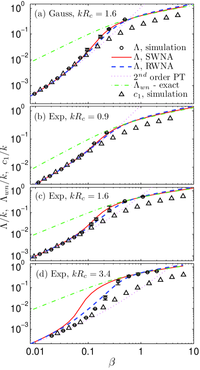
First, we examine models of disorder with the quickly decaying exponential and Gaussian correlation functions (Table 1). The results are compared to the Monte-Carlo simulation in Fig. 1. The error bars indicate uncertainty of the Monte-Carlo calculation of the generalized LE, which is explained in Appendix C. the generalized LE is plotted for different values of as a function of the dimensionless noise intensity
| (49) |
where is defined in Eq. (9). Note that in the Born approximation (69) for the white noise disorder.
The standard and the regularized white noise approximations yield close results for , while Difference between them increases with and, e.g., for the exponential correlation with , it becomes of the order of ten (Fig. 1(d)). Comparison with the simulation results shows that both approximations are good for (Fig. 1(a-c)), but deteriorate with further increase of , as expected. For example, for the exponential correlation with , the resul of the standard approximation and the simulated values of differ already by a factor of ten at moderately strong disorder, (Fig. 1(d)). The regularized white noise approximation seems to be somewhat better, though the improvement is inconclusive.
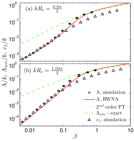
The main advantage of the regularized white noise approximation is its applicability to the long-range correlations, as demonstrated in Fig. 2. As an example, we use ”speckle” correlation function , where , which describes correlation of the intensity in some quasi-one-dimensional laser speckle patterns Goodman-84 . The latter are used to create disordered potentials in experiments with cold atoms Aspect-Speckle-06 . Note, however, that our Gaussian model does not describe a true speckle intensity, which exhibits highly non-Gaussian fluctuations. This correlation function has a remarkable property that the corresponding power spectrum, given by the Fourier transform of the correlation function , is proportional to the ”tent” function and vanishes for . As a results, the Born approximation for both LE and the generalized LE , Eq. (69), vanishes for . In view of this fact, the regularized white noise approximation is tested below and above this threshold for equal to and respectively. In both cases we find agreement with the simulation results within the factor of the order of unity (Fig. 2).
Let us summarize the above comparison of the analytical and the numerical results. The suggested simple regularization allows extension of the standard white noise closure approximation to the cases of slowly decaying correlations. In the regime of moderate disorder, , white noise approximation is applicable for (we consider ), in accord with the formal requirement (cf. Eq. (35)). In the limit of weak disorder, , our approximation coincides with the perturbation theory (69), i.e. becomes exact up to weak disorder corrections. Thus, for , the validity condition is relaxed (cf. discussion after Eq. (38)). Finally, for strong disorder, , numerical data coincide with and, thus, confirm the analytical result , obtained for , i.e. , at the end of Sec. III.3. This is inspite of the fact that for in our simulations we have , which violates the white noise approximation validity condition , Eq. (35). In the next section, however, the same relation is obtained in the regime specifically for Gaussian disorder.
IV Semiclassical regime of strong disorder
In this section we analytically calculate cumulant coefficients , defined by Eq. (12), in the regime when conditions and are fulfilled, where is the noise variance introduced in Eq. (6). An opposite regime, , corresponds to the white noise limit, for which the cumulants were calculated in Ref. Schomerus-02 . We assume that and are typical height and width of the random barriers, therefore probability of a tunneling through a single typical barrier is exponentially small under the above conditions. In this case, as argued in Ref. Deych-03 , transport is dominated by the under-barrier tunneling and interference effects are negligible. Since is a spatial scale of the disorder , the second condition, , justifies the semiclassical approximation for the under-barrier tunneling. Thus, an exponential growth rate of the solution amplitude can be estimated as a magnitude of the imaginary part of the semiclassical action:
| (50) |
Here is an imaginary part of the complex momentum, where is a short notation for the unit step function. Function selects regions where the energy is below the disorder barriers and solution grows exponentially, while the remaining regions, where has an oscillatory behavior, are discarded.
Semiclassical approximation (50) directly relates distribution of to the statistical properties of the above-threshold excursions of the random process . Disorder average of Eq. (50) yields LE or the first cumulant coefficient
| (51) |
where is a conditional average for over the distribution . Here is distribution of the disorder values at a single position.
Using semiclassical approximation (50), higher cumulant coefficients can be expressed in terms of the corresponding joint cumulants of :
| (52) |
Since is a stationary process, the joint cumulants in Eq. (52) depend only on the coordinate difference. The value of the cumulants is maximal when all the coordinates coincide, and decays on the scale with a distance between the points. This is because is the only spatial scale in our model (6). Thus, shifting all the coordinates in the cumulant by and assuming , the integral in (51) can be approximated as
| (53) |
where we have neglected the boundary effects at the corners and extended the integration to . For the Gaussian process , an analytical calculation of the joint cumulants of is quite involved. It is, however, possible to obtain a simple estimate of the multiple integral in (53). As an example, consider the two-point correlator of the regular step function , which can be calculated analytically Blacknell-01 , and is given by
| (54) |
where the dimensionless correlation function was defined in Eq. (6). As expected, the two-point correlator of decays in the same manner as . Due to the normalization conditions (7), the integral of the expression in Eq. (54) is of the order of . Similarly, any -order cumulant in (53) has maximum value and decays with a distance from the origin on the scale . Therefore, rescaling the integration variables in (53) by , the remaining dimensionless integral can be grossly estimated as a volume of the -dimensional unit sphere . This gives the following estimate
| (55) |
where functions are of the order of unity (according to Eq. (51), ), and , which is independent of the position . Coefficients compensate for the approximation of the -dimensional integral by the volume of sphere and depend weakly on the specific form of the correlation function of and on the ratio . Numerical values of can be found in computer simulation by calculating statistics of the quantity on the right hand side of Eq. (50), and fitting it to Eq. (55). As an example, we obtain , and , for all three types of correlations given in Table 1.
Combining Eqs. (51) and (55), one obtains the following relations
| (56) |
where are dimensionless functions, whose specific form depends only on the disorder distribution . This result should be contrasted with the weak disorder relations (4).
Using the fact that is either or , it is convenient to express cumulants of in terms of and , where denotes a ”conditional cumulant”, calculated with distribution [see Appendix D]. For example, for one obtains
| (57) |
This expansion is helpful, since it shows separate contributions of the fluctuation of the indicator function and of the barrier height fluctuation above the level .
Finally, the semiclassical approximation (50) can be used to calculate the generalized LE in strong disorder limit
| (58) |
where the disorder average of the exponential involves functional integration over . As an example, we calculate for Gaussian disorder in the limit and , which justifies the stationary point approximation. The latter yields
| (59) |
According to Eqs. (59) and (78), under the conditions and , LE ratio scales like . For comparison, the Gaussian part of , i.e. [cf. Eq.(16)], scales in this regime as . The obtained scaling is closely related to the statistics of the disorder fluctuations and, thus, is specific to the considered Gaussian models (e.g., for strong binary disorder one expects ).
Let us note that in Eq. (59) matches very closely the strong disorder limit of the small- approximation for (Sec. III.3, last paragraph). The latter reads , where and is the generalized LE for -correlated disorder in strong disorder limit (cf. Eq.(64)). The semiclassical result (59) gives , which is remarkably close to the small- approximation. Note that the considered limit, , implies that , which is formally beyond validity of the small- approximation.
 |
 |
 |
 |
V Transmission Statistics
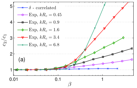
In this section we discuss properties of the transmission coefficient distribution in terms of the dimensionless ratios , and , Eqs. (13) and (16). The cumulant coefficients are simulated numerically for three types of correlations listed in Table 1 and for the white noise model as well. For the generalized LE we use both analytical and numerical results. Details of the numerical simulations are given in Appendix C. All calculations are performed at the same fixed value of energy, , and for different values of the correlation radius and the disorder variance . Disorder strength is conveniently characterized by the dimensionless disorder intensity , introduced in Eq. (49). For each considered value of , quantities and are studied as a function of in the range from weak () to strong () disorder.
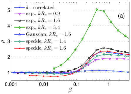
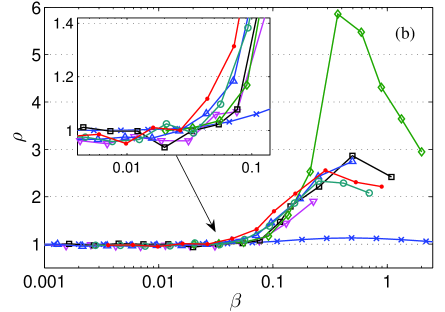
In Figs. 3 and 4 we plot and cumulant ratios and respectively as a function of . Different data series correspond to different models of correlation and different fixed values of , as indicated in the legends. All three quantities, , and , exhibit qualitatively similar behavior in weak and moderate disorder (). As expected from the results on the -correlated disorder Pikovsky-03 ,Schomerus-02 , universal relations , and (cf. Eqs.(4) and (16)) are violated beyond weak disorder. Our calculations show that deviation from these weak disorder values is strongly enhanced in the presence of correlations and increases with the correlation radius . Namely, while this deviation is small compared to unity for -correlated disorder, it becomes of the order of unity, or even larger, in the presence of correlations. Below we discuss the obtained results and the corresponding parametric dependences.
 |
 |
 |
 |
V.1 Scaling of the cumulant ratios
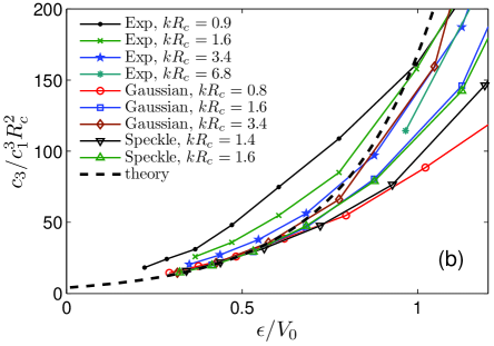
In sufficiently strong disorder, such that , cumulant ratios are described by the semiclassical relations (56). To verify these relations, in Fig. 5 we plot for , as a function of and compare it to the semiclassical prediction , according to Eq. (56). For Gaussian disorder, functions are given by Eq. (79), and we use values and , as explained in text after Eq. (57). Fig. 5 shows that the obtained numerical values converge to the theoretical curve for . As expected, the semiclassical approximation improves for smaller and larger . Let us note, for clarity, that in our presentation we increase the disorder amplitude keeping fixed and fixed . In this parametrization, cumulant ratios grow monotonically with , roughly as (cf. Fig. 4). If, however, relative disorder strength is increased by decreasing at fixed and , then ratios would eventually vanish for sufficiently large and negative , as can be seen from Eq. (56) [because becomes small in this limit].
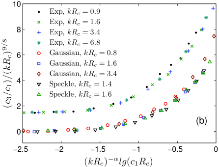
Semiclassical scaling (56) is not applicable in weak and moderate disorder. In this regime, and for , we find empirically that deviation from the weak disorder relations (4) for is described by the following approximate scaling
| (60) |
where is the Kronecker delta. Here are some dimensionless monotonically increasing functions, whose form depend on the type of correlation. Exponent is not universal as well, and we find that , for the exponential, and for the Gaussian and the speckle correlation functions (Table 1). On the contrary, in the considered Gaussian models, we obtain and , irrespectively of the disorder correlation. In Fig. 6 we plot and against , which demonstrates that scaling (60) holds for a rather broad range of the considered values of (see legends) as long as . A logarithmic scale plot of , given in the inset of the upper panel, shows that this scaling holds also at small values of (the same is true also for ).
Let us stress that relations (60) become meaningless in the white noise limit , and are applicable only for , when deviation from the weak disorder relations (4) is dominated by the effects of the correlations. According to Eq. (60), the latter is controlled by the ratio of the correlation to the localization lengths, .
As seen in Fig. (6), functions are rather similar, though not identical, for different models of correlation. The major distinction in a specific form of relation (60) for different (Gaussian) models appears in the value of the exponent . It is interesting to note that both and practically coincide for the models with Gaussian and speckle correlation functions. This can be related to the qualitative similarity of their power spectra, given by the Gaussian and the ”tent” function respectively, which have either effective or exact cutoff of the order of (the ”tent” function, , was introduced in Sec. III.5). On the contrary, power spectrum of the exponentially correlated disorder is given by the slowly decaying Lorentzian function. Note that disorder power spectrum appears, e.g., in the Born approximation (69) for (and LE ), which shows close relation between the properties of localization and those of the disorder power spectrum.
V.2 Extreme fluctuation of
Beyond weak disorder, LE ratio increases with the correlation parameter and, as a function of the disorder intensity, exhibits a peak Note-peak-of-rho at moderate disorder (Fig. 3). Thus, as expressed in terms of the ratio between the mean and the typical values of the inverse transmission coefficient , Eq. (17), also the extreme relative fluctuation of is peaked at moderate disorder and is enhanced by the disorder correlations. This conclusion is consistent with our observation that statistical convergence of the Monte-Carlo simulation of the generalized LE is most slow at moderate disorder and for larger values of , as indicated by the error bars in Figs. 1 and 2. Note that relative fluctuation (17) depends exponentially on , where . Therefore, for and , correlations lead to the exponentially large enhancement of the extreme fluctuation of as compared to the case of the -correlated disorder.
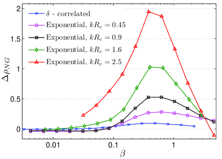
It is instructive to compare to its Gaussian part . The latter is obtained by discarding the non-Gaussian terms, , in Eq. (16), which is equivalent to approximating the asymptotic distribution of by the Gaussian one with the same mean and variance, equal to and respectively. Correspondingly, contribution of the non-Gaussian corrections is represented by the difference . In Fig. 7 we plot for the -correlated and the exponentially correlated disorder (other models of correlation exhibit similar behavior). In agreement with relations (4), vanishes in the weak disorder limit. Beyond this regime, is positively peaked at moderate disorder, and the magnitude of the peak increases with . Positive values of mean that the low- tail of the -distribution is heavier than in the Gaussian approximation in a sense that and, thus, the relative fluctuation (17), are larger than in the corresponding Gaussian distribution. The result in Fig. 7 shows that this ”super-Gaussian” effect is enhanced by the disorder correlations and is most prominent at moderate disorder. Let us stress, however, that this statement applies only to the integral quantity (17) and does not imply any specific form (e.g., super- or sub-Gaussian) for the asymptotic decay law of the low- tail in the -distribution. The latter was studied , e.g., in Refs. Pikovsky-03 , Opt-Fluct , Raikh using different methods.
VI Conclusions
We have considered statistical properties of the transmission coefficient of a one-dimensional disordered system described by the Schrödinger Eq. (1) with a Gaussian correlated disorder. The main focus of our study was an effect of the correlations on the transmission distribution, which was characterized in terms of the dimensionless ratio between the generalized and the usual Lyapunov exponents, , as well as ratios and of the asymptotic cumulants of . Both analytical and numerical methods were employed for calculation of and .
First, a small- approximation was developed for the generalized LE , which is not limited to weak disorder and also is able to account for the non-trivial effects of the correlations. To this end, we obtained an infinite hierarchy of integro-differential equations on the second moments of the wave function and its functional derivatives with respect to the disorder. We have shown that this hierarchical chain can be truncated starting from the second level to obtain a non-trivial approximation, which accounts for the correlations of the disorder. Note that termination of this hierarchy on the first level accounts only for the intensity of the noise, while all information on the correlation properties is lost. This non-trivial closure allowed us to obtain an analytical solution for the generalized LE in an implicit form as a largest real root of a non-linear algebraic equation. The obtained approximation is valid formally for and , where is the wave number. It turned out that a standard white noise approximation Klatzkin does not allow to treat the generalized LE in the case of sub-exponentially decaying correlations. To overcome this obstacle, we have proposed a simple self-consistent regularization, which extends the applicability of the approximation to any correlation function satisfying . The derived small- approximation was compared to numerical simulations and a good agreement was found.
The asymptotic cumulants of were calculated analytically within the semiclassical approximation applicable in a special case of strong disorder, and . For an arbitrary strength of disorder, cumulant coefficients were obtained by numerical simulations.
Using these analytical and numerical methods, the generalized LE and the first three cumulants of were calculated for several models of correlations and for different values of , which enabled us to investigate effects of correlations on the form of the transmission distribution. In order to study transition between the regimes of weak and strong disorder, we have considered only positive energies , where it was convenient to introduce the dimensionless disorder intensity , defined in Eq. (49).
In sufficiently weak disorder, we obtained , and in all the considered cases. Thus, as expected from previous work (e.g., Refs. Tamura-93 ,Petri-96-97 ,Zaslavsky-97 ,Deych-03 ), in weak disorder, correlations do not destroy SPS and do not modify the universal relations (4). In the white noise limit, , this regime is realized for . For , the relevant control parameter is the ratio of the correlation to the localization lengths, . Quantity is interpreted naturally as a measure of randomization of the disorder potential on the scale of the localization length. Correspondingly, the weak disorder universality, expressed by relations (4), takes place when (for , this means that disorder is weak also in the conventional sense ).
Relations (4) are not valid beyond weak disorder. In the white noise model, the corresponding deviation from these relations is weak for any strength of the disorder (for ), in a sense that values of and stay very close to unity, while remains small compared to unity. On the contrary, in correlated disorder, these quantities depend strongly on the strength of the disorder through the control parameter . Regarding this parametric dependence, we discuss two regimes: and .
The first regime, , corresponds to transition from weak to moderate disorder. In this regime and for , cumulant ratios and are described by the approximate scaling relations (60) with parameters and . This relations demonstrate that, starting from weak disorder (), ratios increase gradually with parameter and, for , arrive at values which can be much larger than unity (depending on ). In such a case, the bulk of the -distribution becomes much broader than in weak or in the white noise disorder.
While the small- cumulant coefficients describe bulk of the -distribution, LE ratio is a measure of the extreme relative fluctuation of , expressed by the ratio between the mean and the typical values of , Eq. (17). Like the cumulant ratios, increases from weak to moderate disorder and its deviation from the weak disorder value is strongly enhanced by the disorder correlations (namely, exceeds unity for ). As a function of the disorder strength, and, thus, the extreme relative fluctuation (17), are peaked at moderate disorder (near ). This peak of is associated with the non-Gaussian corrections to the low- tail of the -distribution, whose contribution to is positively peaked, i.e. ”super-Gaussian”, at moderate disorder. The latter has the following simple interpretation in terms of the disorder statistics. In moderate disorder, when energy is of the order of , wave propagation becomes affected by the under-barrier tunneling through the rare but large peaks of the random potential. For, already a single large barrier becomes a strong scatterer. Therefore, fluctuations in height and in occurrence of these rare peaks lead to extreme deviations of from its typical value. In stronger disorder, the typical value grows significantly, and relative contribution of the large rare barriers becomes less pronounced. This simple explanation can be confirmed by calculating in the framework of the semiclassical approximation (50) [not presented here].
The second regime, , is realized when and . In these conditions, interference effects are suppressed and localization is dominated by under-barrier tunneling. Then, according to Eq. (50), the transmission distribution is directly related to the statistics of the ”excursions” of the random potential above the level , and the cumulants of satisfy the ”semiclassical” scaling relations (56), which were verified in numerical simulations. According to Eq. (56), the effect of correlations is expressed by the simple relation , where the coefficient depends only on the one-point distribution of disorder. Semiclassical approximation can also be used to calculate the generalized LE . In particular, for and , we obtain scaling , which is specific to Gaussian statistcs of disorder.
Acknowledgements.
We are grateful to B. Shapiro for useful discussions. This work was supported by the Israel Science Foundation under the grants No. 1067/06 and 1299/07.Appendix A Exact solution for in -correlated disorder
Equation (23) decouples and can be solved exactly for the -correlated disorder (see e.g. Ref. Pikovsky-03 ). Namely, substituting into (23) and using the initial condition (27), one obtains
| (61) |
where
| (62) |
and matrices and are defined in (21). Solution of Eq. (61) is
| (63) |
where is an initial condition. The generalized LE , Eq. (14), is given by the largest real eigenvalue of the matrix . It is found from the cubic equation
| (64) |
which has the following roots
| (65) |
where . The generalized LE is given by , which is real and positive. Other two eigenvalues are complex for (i.e. ), and real otherwise. Matrix is not normal (), and its left and right eigenvectors, corresponding to the eigenvalues in Eq. (65), are
| (66) |
These eigenvectors satisfy the normalization .
Appendix B Born approximation for
The systematic weak disorder expansion (i.e. in powers of the disorder amplitude ) for the generalized LE was considered in Ref. Tessieri-02 . Here we only note that the Born approximation for can be obtained by substitution of the zero order solution for into (23). The zero order solution for is obtained by neglecting the noise term in equation (26):
which has the solution
| (67) |
Inserting this solution into Eq. (23) yields an equation closed with respect to :
| (68) |
where pair correlation function is defined in Eq. (6). Then, lowest order calculation of the asymptotic growth rate of the solution yields the Born approximation
| (69) |
where and . This expression coincides with the Born approximation for LE LGP-Introduction .
Appendix C Method of numerical simulations
The numerical simulations were performed using the tight-binding (TB) model
| (70) |
with energy near the band edge, , and the diagonal disorder . In this regime, Eq. (70) is a good approximation to the continuous model (5). We relate the continuous model with energy and potential to the TB counterpart by setting
| (71) |
The correlated Gaussian disorder was generated by filtering sequences of independent Gaussian random variables. The real space convolution with a proper kernel was used to obtain the ”short-range” exponential () and Gaussian () correlations, while the Fourier space filter was applied to obtain the power law correlation .
In all simulations presented in this paper, we have fixed the energy at and varied values of the disorder amplitude and the correlation radius . Note that for , the corresponding wavelength of the solution for a pure system () is equal to about sites. Therefore, approximation to a continuum is good as long as .
A standard transfer matrix formalism (see e.g. Ref. Liu-86 ) was used, in which the TB equation (70) is rewritten in the matrix form
| (72) |
where is a single-site transfer matrix. Then, solution of the initial value problem is given by
| (73) |
where is the total transfer matrix for the system of length .
In analogy with Eq. (19), one can introduce vector , where and . Similarly to (73), the solution for can be write as
| (74) |
where is an initial condition, and is the transfer matrix for , which is readily expressed in terms of the elements of . The largest eigenvalue of is equal to the square modulus of the largest eigenvalue of . Finally, ensemble average over the disorder realizations yields
Cumulant coefficients , defined in Eq. (12), are given by the asymptotic linear growth rate of the cumulants with the system length , where denotes the largest eigenvalue of the matrix . The asymptotic slope was calculated by the linear fit, which have to exclude the region of the initial transient of the order of a few localization lengths. The ensemble average was performed over realizations of disorder.
The generalized Lyapunov exponent , Eq. (14), was calculated as a linear slope of . Alternatively, could be found as a slope of the logarithm of the largest eigenvalue of , which gives practically the same result. About realization were generated to calculate each value of .
Monte-Carlo simulation of the generalized LE can be a quite challenging task, as is briefly explained in the following. In numerical simulation of the generalized LE one have to deal with two restrictions on the system size, both from below and from above. The lower bound is determined by the width of the transient to the asymptotic behavior
| (75) |
Width of this transient is at least of the order of . This follows from the form of the differential equation (23) for , which suggests that growth rate of can not stabilize unless . This is because the correlation function in the integral on the right hand side of Eq. (23) decays on the scale of . In the white noise limit, , the transient region is absent, as follows from the exact analytical result (Appendix A) and was observed numerically. Therefore, we assume that the width of the transient is of the order of , and other scales, such as the localization length, are less important (unlike the case of , ).
The upper bound on the system size is determined empirically from the numerical data as a value of , beyond which the linear dependence in Eq. (75) is violated. This computational artifact originates from the insufficient statistics in averaging of the broadly distributed quantity , which is equivalent to . According to Eqs. (2) and (4), distribution of is log-normal in weak disorder, while some corrections to the limiting log-normal form appear in stronger disorder. As follows from Eqs. (13) and (17), this distribution becomes increasingly broad and heavy-tailed with the increase of the dimensionless system length . For large , long tails of the distribution, which dominate the theoretical mean of , are typically under-sampled in simulations with a finite number of realization. As a result, the obtained values of become typically underestimated (formally, expectation value of becomes smaller that , where is the theoretical mean). This effect increases with the system size, the relevant length scale being the localization length . Therefore, the upper bound on the system length is of the order of a few . Thus, the upper and the lower bounds eventually coincide in sufficiently strong disorder, since becomes small. In such a case, numerical calculation of becomes impossible, unless the number of the realizations is increased dramatically (for the exactly log-normal , it can be shown that the improvement is logarithmically slow). In moderate disorder, the small range between the lower and the upper bounds results in large uncertainty in the calculated , as indicated by the error bars in Figs. 1 and 2.
Appendix D Auxiliary formulas for semiclassical approximation
Cumulants are easily written in terms of and using that and , where stands for the average with the distribution , introduced in Sec. IV. For example, the second cumulant, , becomes
| (76) |
which, using and , yields after some rearrangement
| (77) |
Similar expansion for the third cumulant, , gives expression (57) for .
For Gaussian distribution , definition (51) yields the following expression for LE:
| (78) |
while functions for are given by ()
| (79) |
where is a confluent hypergeometric function of the second kind (or Tricomi function) and is a modified Bessel function of the second kind Abramovich .
References
- (1) P. Hänggi and P. Jung, Adv. Chem. Phys. 89, 239 (1995).
- (2) P.W. Anderson, Phys. Rev. 109, 1492 (1958).
- (3) R. Zillmer and A. Pikovsky, Phys. Rev. E 67 061117 (2003).
- (4) I.M. Lifshitz, S.A. Gredeskul, and L.A. Pastur, Introduction to the Theory of Disordered Systems (Wiley, New York, 1988).
- (5) H. Schomerus and M. Titov, Phys. Rev. E 66, 066207 (2002).
- (6) G. Paladin and A. Vulpiani, Phys. Rev. B 35, 2015 (1987).
- (7) S. Kotani, Proceedings of Conference on Stochastic Analysis Kyoto, (1982).
- (8) B. Simon, Commun. Math. Phys. 89, 227 (1983).
- (9) S. Kotani and B. Simon, Commun. Math. Phys. 112, 103 (1987).
- (10) L. Pastur and A. Figotin, Spectra of Random and Almost-Periodic Operators, Springer-Verlag, Berlin (1992).
- (11) R. Landauer, Philos. Mag. 21, 863 (1970).
- (12) D. S. Wiersma et al., Nature 390, 671673 (1997); T. Schwartz et al., Nature 446, 5255 (2007); Y. Lahini et al., Phys. Rev. Lett. 100, 013906 (2008).
- (13) A. A. Chabanov, M. Stoytchev, and A. Z. Genack, Nature (London) 404, 850 (2000) ; U. Kuhl, F.M. Izrailev, A.A. Krohin, and H.-J. Stockmann, Appl. Phys. Lett. 77, 633 (2000).
- (14) J. Billy, V. Josse, Z. Zuo, A. Bernard, B. Hambrecht, P. Lugan, D. Clément, L. Sanchez-Palencia, P. Bouyer, and A. Aspect, Nature (London) 453, 891 (2008); G.Roati, C. D’Errico, L. Fallani, M. Fattori, C. Fort, M. Zaccanti, G. Modugno, M. Modugno, and M. Inguscio, Nature 453, 895 (2008).
- (15) H. Hu, A. Strybulevych, J. H. Page, S. E. Skipetrov, and B. A. van Tiggelen, Nature Physics 4, 945 (2008).
- (16) T. Ernst, T. Paul, P. Schlagheck, Phys. Rev. A 81, 013631 (2010).
- (17) D. Clément, A.F. Varon, J.A. Retter, L. Sanchez-Palencia, A. Aspect and P.Bouyer, New J. Phys. 8, 165 (2006).
- (18) F.M. Izrailev and A.A. Krokhin, Phys. Rev. Lett. 82, 4062 (1999).
- (19) L. Tessieri and F. M. Izrailev, Phys. Rev. E 64, 66120 (2001).
- (20) E. Gurevich and O. Kenneth, Phys. Rev. A 79, 063617 (2009).
- (21) P. Lugan, A. Aspect, L. Sanchez-Palencia, D. Delande, B. Grémaud, C.A. Müller, and C. Miniatura, Phys. Rev. A, 80, 023605 (2009).
- (22) L. Tessieri, J.Phys. A: Math. Gen. 35, 9585 (2002).
- (23) A. Iomin, Phys. Rev. E 79, 062102 (2009).
- (24) M. Titov and H. Schomerus, Phys. Rev. Lett. 95, 126602 (2005).
- (25) L. I. Deych, M. V. Erementchouk, and A. A. Lisyansky, Phys. Rev. B 67, 024205 (2003).
- (26) D. H. Dunlap, H. L. Wu, and P. W. Phillips, Phys. Rev. Lett. 65, 88 (1990) ; F. A. B. F. de Moura and M. L. Lyra, Phys. Rev. Lett. 81, 3735 (1998); T. Kaya, Eur. Phys. J. B 55, 49 (2007); A.M. Garcia-Garcia and E. Cuevas, Phys. Rev. B 79, 073104 (2009).
- (27) P. W. Anderson, D.J. Thouless, E. Abrahams and D.S. Fisher, Phys. Rev. B 22, 3519 (1980).
- (28) A. Cohen, Y. Roth and B. Shapiro, Phys. Rev. B 38, 12125 (1988).
- (29) B. Shapiro, Philos. Mag. B 56, 1031 (1987).
- (30) M. J. de Oliveira and A. Petri, Phys. Rev. E 53, 2960 (1996); Phys. Rev. B 56, 251 (1997).
- (31) A.A. Abrikosov, Solid State Commun. 37, 997 (1981).
- (32) L. I. Deych, A. A. Lisyansky, and B. L. Altshuler, Phys. Rev. Lett. 84, 2678 (2000); Phys. Rev. B 64, 224202 (2001).
- (33) N. Nishiguchi, S. I. Tamura, and F. Nori, Phys. Rev. B 48, 2515 (1993); 48, 14426 (1993).
- (34) L. I. Deych, D. Zaslavsky, and A. A. Lisyansky, Phys. Rev. E 56, 4780 (1997).
- (35) H. Schomerus and M. Titov, Phys. Rev. B 67, 100201(R) (2003).
- (36) V.I. Kliatskin, Stochastic equations and waves in randomly inhomogeneous media (Nauka, Moskva, 1980) (in Russian).
- (37) P.A. Mello and N. Kumar, Quantum transport in mesoscopic systems: complexity and statistical fluctuations, (Oxford University Press, Oxford, 2004).
- (38) Correlation between the transmission coefficient and the reflection and transmission phases is not exactly zero, and it can not be ignored in certain circumstances. One such example is calculation of the transmission (conductance) distribution based on the phase formalism Schomerus-03 . For our purposes, however, this correlation becomes negligible in the limit of long system.
- (39) R. A. Horn and C. R. Johnson, Matrix Analysis (Cambridge University Press, New York, 1985).
- (40) J.W. Goodman, ”Statistical properties of Laser Speckle Patterns” in ”Laser Speckle and Related Phenomena”, edited by J.C. Dainty, 2nd Ed., Springer-Verlag 1984.
- (41) D. Blacknell, M. Jahangir, F. Piccoloand, R. J. A. Tough, J. Phys. A: Math. Gen. 34, 1231 (2001).
- (42) According to our semiclassical treatment of strong disorder (Sec. IV, Eq. (59)), scales as for and . Thus, if is increased with and fixed, then the local peak of at moderate disorder is followed by subsequent increase at much stronger disorder. The latter is not present in Fig. 3, which corresponds to less strong disorder, . In fact, we checked that the non-monotonic dependence of on in moderate and strong disorder can be obtained using the semiclassical approximation (50).
- (43) I.E. Smolyarenko, B.L. Altshuler. Phys. Rev. B 55, 10451 (1997).
- (44) V.M. Apalkov, M.E. Raikh, Semiconductors 42, 940 (2008).
- (45) Y. Liu and K.A. Chao, Phys. Rev. B 34, 5247 (1986).
- (46) M. Abramowitz and I. Stegun, Handbook of Mathematical Functions with Formulas, Graphs, and Mathematical Tables (Dover Publications, New York , 1972).