Factorizations and Reductions of Order in Quadratic and other

Non-recursive Higher Order Difference Equations

H. SEDAGHAT*

Abstract. A higher order difference equation may be generally defined in an arbitrary nonempty set ${\small S}$ as:

$$f_{n}(x_{n},x_{n-1},\ldots,x_{n-k})=g_{n}(x_{n},x_{n-1},\ldots,x_{n-k})$$

where ${\small f}_{{\small n}}{\small,g}_{{\small n}}{\small:S}^{k+1}{\small\rightarrow S}$ are given functions for ${\small n=1,2,\ldots}$ and ${\small k}$ is a positive integer. We present conditions that imply the above equation can be factored into an equivalent pair of lower order difference equations using possible form symmetries (order-reducing changes of variables). These results extend and generalize semiconjugate factorizations of recursive difference equations on groups. We apply some of this theory to obtain new factorization results for the important class of quadratic difference equations on algebraic fields:

$$\sum_{i=0}^{k}\sum_{j=i}^{k}a_{i,j,n}x_{n-i}x_{n-j}+\sum_{j=0}^{k}b_{j,n}x_{n-j}+c_{n}=0.$$

We also discuss the nontrivial issue of the existence of solutions for quadratic equations.

1 Introduction

Let $S$ be a nonempty set and $\{f_{n}\}_{n=1}^{\infty},\{g_{n}\}_{n=1}^{\infty}$ be sequences of functions $f_{n},g_{n}:S^{k+1}\rightarrow S$ where $k$ is a positive integer. We call the equation

$$f_{n}(x_{n},x_{n-1},\ldots,x_{n-k})=g_{n}(x_{n},x_{n-1},\ldots,x_{n-k}),\quad n=1,2,3,\ldots$$ (1)

a non-recursive difference equation of order $k$ in the set $S$ if $f_{n}(u_{0},\ldots,u_{k})$ is not constant in $u_{0}$ and $g_{n}(u_{0},\ldots,u_{k})$ is not constant in $u_{k}$ for all $n\geq 1.$ A (forward) solution of (1) is a sequence $\{x_{n}\}_{n=1}^{\infty}$ in $S$ that makes (1) true, given a set of initial values $x_{-j}$, $j=0,1,\ldots,k-1.$ The recursive, non-autonomous equation of order $k,$ i.e.,

$$x_{n}=\psi_{n}(x_{n-1},\ldots,x_{n-k})$$ (2)

is a special case of (1) with

$$f_{n}(u_{0},u_{1},\ldots,u_{k}) =u_{0}$$

$$g_{n}(u_{0},u_{1},\ldots,u_{k}) =\psi_{n}(u_{1},\ldots,u_{k})$$

for all $n$ and all $u_{0},u_{1},\ldots,u_{k}\in S.$

An example of non-recursive equations in familiar settings is the following on the set $\mathbb{R}$ of all real numbers:

$$|x_{n}|=a|x_{n-1}-x_{n-2}|,\quad 0<a<1$$ (3)

This states that the magnitude of a quantity $x_{n}$ at time $n$ is a fraction of the difference between its values in the two immediately preceding times; however, we cannot determine the sign of $x_{n}$ from (3). As a possible physical interpretation of (3) imagine a node in a circuit that in every second $n$ fires a pulse $x_{n}$ that may go either to the right (if $x_{n}>0$) or to the left (if $x_{n}<0$) but the amplitude $|x_{n}|$ of the pulse obeys Eq.(3). With regard to the variety of solutions for (3) we note that the direction of each pulse is entirely unpredictable, regardless of the directions of previous pulses emitted by the node; hence a large number of solutions are possible for (3). We discuss this equation in greater detail in the next section.

For recursive equations such as (2) on groups, recent studies such as [7], [11], [12], [13], [14], [15], [17], [18], show that possible form symmetries (i.e., order-reducing coordinate transformations or changes of variables) and the associated semiconjugate relations may be used to break down the equation into a triangular system [20] of lower order difference equations whose orders add up to the order of (2). But in general it is not possible to write (1) in the recursive form (2) so the question arises as to whether the notions of form symmetry and reduction of order can be extended to the more general non-recursive context.

In this paper, we show that for Eq.(1) basic concepts such as form symmetry and factorization into factor and cofactor pairs of equations can still be defined as before, even without a semiconjugate relation. A concept that is similar to semiconjugacy but which does not require the unfolding map is sufficient for defining form symmetries and deriving the lower order factor and cofactor equations. Using this idea we extend previously established theory of factorization and reduction of order to a much larger class of difference equations then previously studied. In particular, we apply this extended theory to the important class of quadratic difference equations.

2 Factorizations of non-recursive equations

Equation (1) generalizes the recursive equation (2) in a different direction than the customary one, namely, through unfolding the recursive equation of order $k$ to a special vector map of the $k$-dimensional state-space $S^{k}$. Nevertheless, it is convenient to define as states the points $(x_{n},x_{n-1},\ldots,x_{n-k+1})\in S^{k}$ or some invariant subset of it that contains the orbit

$$\{(x_{n},x_{n-1},\ldots,x_{n-k+1})\}_{n=1}^{\infty}$$

of every solution $\{x_{n}\}_{n=1}^{\infty}$ of (1). We may designate the point $(x_{0},\ldots,x_{-k+1})$ corresponding to $n=0$ on each orbit as the “initial point” of that orbit; in contrast to recursive equations however, there may be many distinct orbits having the same initial point.

Analyzing the solutions of a non-recursive difference equation such as (1) is generally more difficult than analyzing the solutions of recursive equations. Unlike the recursive case, even the existence of solutions for (1) in a particular set is not guaranteed. But studying the form symmetries and reduction of order in non-recursive equations is worth the effort. The greater generality of these equations not only leads to the resolution of a wider class of problems, but it also provides for increased flexibility in handling recursive equations.

Before beginning the formal study of factorizations of non-recursive equations, let us consider an illustrative example that highlights several issues pertaining to such equations.

Example 1

Let $\{a_{n}\}_{n=1}^{\infty}$ be any sequence of non-negative real numbers and consider the following third-order difference equation on $\mathbb{R}$:

$$|x_{n}+x_{n-1}|=a_{n}|x_{n-1}-x_{n-3}|.$$ (4)

By adding and subtracting $x_{n-2}$ inside the absolute value on the right hand side of (4) we find that

$$|x_{n}+x_{n-1}|=a_{n}|x_{n-1}+x_{n-2}-(x_{n-2}+x_{n-3})|$$ (5)

The substitution

$$t_{n}=x_{n}+x_{n-1}$$ (6)

in (5) results in the second-order difference equation

$$|t_{n}|=a_{n}|t_{n-1}-t_{n-2}|$$ (7)

that is related to (4) via (6). Eq.(7) is analogous to a factor equation for (4) while (6), written as

$$x_{n}=t_{n}-x_{n-1}$$ (8)

is analogous to a (recursive) cofactor equation. Also the substitution (6) is analogous to an order-reducing form symmetry; see, e.g., [12], [13], [14] or [18].

The factor equation (7) is of course not recursive; it is a generalization of (3) in the introduction above. If $\{\beta_{n}\}_{n=1}^{\infty}$ is any fixed but arbitrary binary sequence taking values in $\{-1,1\}$ then every real solution $\{s_{n}\}_{n=1}^{\infty}$ of the recursive equation

$$s_{n}=\beta_{n}a_{n}|s_{n-1}-s_{n-2}|$$ (9)

is also a solution of (7). This follows upon taking the absolute value to see that $\{s_{n}\}_{n=1}^{\infty}$ satisfies Eq.(7). The single non-recursive equation (7) has as many solutions as can be generated by each member of the uncountably infinite class of equations (9) put together. Numerical simulations and other calculations indicate a wide variety of different solutions for (9) with different choices of $\{\beta_{n}\}_{n=1}^{\infty}$ and clearly no less is true about (4).

These facts remain true in the special case mentioned in the Introduction, i.e., equation (3) in which the sequence $a_{n}=a$ is constant. By way of comparison first consider the case where $\beta_{n}=1$ is constant for all $n.$ Then each solution $\{s_{n}\}_{n=1}^{\infty}$ of the recursive difference equation

$$s_{n}=a|s_{n-1}-s_{n-2}|,\quad 0<a<1$$

is uniquely defined by an initial point $(s_{0},s_{-1})\in\mathbb{R}^{2}$ and

$$\lim_{n\rightarrow\infty}s_{n}=0.$$ (10)

This claim is proved as follows. Without loss of generality assume that $s_{0}\geq 0$ and define

$$\mu=\max\{s_{0},s_{1}\}\geq 0.$$

Then

$$s_{2} =a|s_{1}-s_{0}|\leq a\max\{s_{0},s_{1}\}\leq a\mu,$$

$$s_{3} =a|s_{2}-s_{1}|\leq a\max\{s_{2},s_{1}\}\leq a\mu.$$

Continuing,

$$s_{4} =a|s_{3}-s_{2}|\leq a\max\{s_{3},s_{2}\}\leq a^{2}\mu,$$

$$s_{5} =a|s_{4}-s_{3}|\leq a\max\{s_{4},s_{3}\}\leq a^{2}\mu.$$

This reasoning by induction yields

$$s_{2n},s_{2n+1}\leq a^{n}\mu,\quad\text{for all }n$$

which proves (10).

By contrast, if $\{\beta_{n}\}_{n=1}^{\infty}$ is not a constant sequence then complicated solutions may occur for (3). The computer generated diagram in Figure 1 shows a part of the solution of the difference equation

$$s_{n}=a\beta_{n}|s_{n-1}-s_{n-2}|$$

with parameter values:

$$a =0.8,\quad s_{-1}=s_{0}=1$$

$$\beta_{n} =\left\{\begin{array}[c]{c}-1\quad\text{if }r_{n}<0.45\\ 1\quad\text{if }r_{n}\geq 0.45\end{array}\right.$$

$$r_{n} =3.75r_{n-1}(1-r_{n-1}),\quad r_{0}=0.4.$$

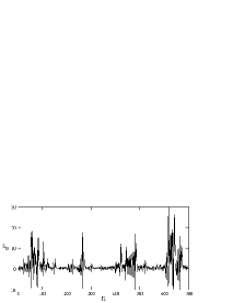
Figure 1: A complex solution of equation (3) highlighting the unpredictability of sign changes

The complex behavior seen in Figure 1 is indicative of the stochastic nature of the pulse direction in the physical interpretation in the Introduction. Although $\{\beta_{n}\}_{n=1}^{\infty}$ does not appear explicitly in (3) the unpredictability of the sign of $x_{n}$ is a way of interpreting the arbitrary nature of the binary sequence.

Finally, we observe that equation (7) which has order two, also admits a reduction of order as follows. If $\{t_{n}\}$ is a solution of (7) that is never zero for all $n$ then we may divide both sides of (7) by $|t_{n-1}|$ to get

$$\left|\frac{t_{n}}{t_{n-1}}\right|=a_{n}\left|1-\frac{t_{n-2}}{t_{n-1}}\right|$$

where the substitution

$$r_{n}=\frac{t_{n}}{t_{n-1}}$$

(analogous to the inversion form symmetry; see [18]) yields the first-order difference equation

$$\left|r_{n}\right|=a_{n}\left|1-\frac{1}{r_{n-1}}\right|.$$ (11)

Eq. (11) is related to (7) via the (recursive) equation

$$t_{n}=r_{n}t_{n-1}.$$ (12)

The factorizations and corresponding reductions in order given by equations (7), (8), (11) and (12) are among the types discussed below along with a variety of other possibilities. For additional examples and further details see [10].

2.1 Form symmetries, factors and cofactors

In this section we define the concepts of order-reducing form symmetry and the associated factorization for Eq.(1) on an arbitrary set $S.$ In analogy to semiconjugate factorizations, we seek a decomposition of Eq.(1) into a pair of difference equations of lower orders. A factor equation of type

$$\phi_{n}(t_{n},t_{n-1},\ldots,t_{n-m})=\psi_{n}(t_{n},t_{n-1},\ldots,t_{n-m}),\quad 1\leq m\leq k-1$$ (13)

may be derived from (1) where $\phi_{n},\psi_{n}:S^{m+1}\rightarrow S$ for all $n$ if there is a sequence of mappings $H_{n}:S^{k+1}\rightarrow S^{m+1}$ such that

$$f_{n}=\phi_{n}\circ H_{n}\text{ and }g_{n}=\psi_{n}\circ H_{n}$$ (14)

for all $n\geq 1.$ If we denote

$$H_{n}(u_{0},\ldots,u_{k})=[h_{0,n}(u_{0},\ldots,u_{k}),h_{1,n}(u_{0},\ldots,u_{k}),\ldots,h_{m,n}(u_{0},\ldots,u_{k})]$$

then for each solution $\{x_{n}\}$ of Eq.(1)

$$\phi_{n}(h_{0,n}(x_{n},\ldots,x_{n-k}),h_{1,n}(x_{n},\ldots,x_{n-k}),\ldots,h_{m,n}(x_{n},\ldots,x_{n-k}))=$$

$$\psi_{n}(h_{0,n}(x_{n},\ldots,x_{n-k}),h_{1,n}(x_{n},\ldots,x_{n-k}),\ldots,h_{m,n}(x_{n},\ldots,x_{n-k}))$$

In order for a sequence $\{t_{n}\}$ in $S$ defined by the substitution

$$t_{n}=h_{0,n}(x_{n},\ldots,x_{n-k})$$

to be a solution of (13), the functions $H_{n}$ must have a special form that is defined next.

Definition 2

A sequence of functions $\{H_{n}\}$ is an order-reducing form symmetry of Eq.(1) on a nonempty set $S$ if there is an integer $m$, $1\leq m<k,$ and sequences of functions $\phi_{n},\psi_{n}:S^{m+1}\rightarrow S$ and $h_{n}:S^{k-m+1}\rightarrow S$ such that

$$H_{n}(u_{0},\ldots,u_{k})=[h_{n}(u_{0},\ldots,u_{k-m}),h_{n-1}(u_{1},\ldots,u_{k-m+1}),\ldots,h_{n-m}(u_{m},\ldots,u_{k})]$$ (15)

and the sequences $\{\phi_{n}\}$, $\{\psi_{n}\},\{f_{n}\},\{g_{n}\}$ and $\{H_{n}\}$ satisfy the relations (14) for all $n\geq 1$.

If $S=(G,\ast)$ is a group then Definition 2 generalizes the notion of recursive form symmetry in [12] where the components of $H_{n}$ are defined as

$$h_{n-j}(u_{j},\ldots,u_{k-m+j})=u_{j}\ast\widetilde{h}_{n-j}(u_{j+1},\ldots,u_{k-m+j}),\quad j=0,1,\ldots,m.$$

We have the following basic factorization theorem for non-recursive difference equations.

Theorem 3

Assume that Eq.(1) has an order-reducing form symmetry $\{H_{n}\}$ defined by (15) on a nonempty set $S.$ Then the difference equation (1) has a factorization into an equivalent system of factor and cofactor equations

$$\phi_{n}(t_{n},\ldots,t_{n-m}) =\psi_{n}(t_{n},\ldots,t_{n-m})$$ (16)

$$h_{n}(x_{n},\ldots,x_{n-k+m}) =t_{n}$$ (17)

whose orders $m$ and $k-m$ respectively, add up to the order of (1).

Proof. To show the equivalence, we show that for each solution $\{x_{n}\}$ of (1) there is a solution $\{(t_{n},y_{n})\}$ of the system of equations (16), (17) such that $y_{n}=x_{n}$ for all $n\geq 1$ and conversely, for each solution $\{(t_{n},y_{n})\}$ of the system of equations (16) and (17) the sequence $\{y_{n}\}$ is a solution of (1).

First assume that $\{x_{n}\}$ is a solution of Eq.(1) through a given initial point $(x_{0},x_{-1},\ldots,x_{-k+1})\in G^{k+1}.$ Define the sequence $\{t_{n}\}$ in $S$ as in (17) for $n\geq-m+1$ so that by (14)

$$\phi_{n}(t_{n},\ldots,t_{n-m}) =\phi_{n}(h_{n}(x_{n},\ldots,x_{n-k+m}),\ldots,h_{n-m}(x_{n-m},\ldots,x_{n-k}))$$

$$=\phi_{n}(H_{n}(x_{n},\ldots,x_{n-k}))$$

$$=f_{n}(x_{n},\ldots,x_{n-k})$$

$$=g_{n}(x_{n},\ldots,x_{n-k})$$

$$=\psi_{n}(H_{n}(x_{n},\ldots,x_{n-k}))$$

$$=\psi_{n}(t_{n},\ldots,t_{n-m}).$$

It follows that $\{t_{n}\}$ is a solution of (16). Further, if $y_{n}=x_{n}$ for $n\geq-k+m$ then by the definition of $t_{n}$, $\{y_{n}\}$ is a solution of (17).

Conversely, let $\{(t_{n},y_{n})\}$ be a solution of the factor-cofactor system (16), (17) with initial values

$$t_{0},\ldots,t_{-m+1},y_{-m},\ldots y_{-k+1}\in G.$$

We note that $y_{0},y_{-1},\ldots,y_{-m+1}$ satisfy the equations

$$h_{j}(y_{j},\ldots,y_{j-k+m})=t_{j},\quad j=0,-1,\ldots,-m+1.$$

Now for $n\geq 1$, (14) implies

$$f_{n}(y_{n},\ldots,y_{n-k}) =\phi_{n}(H_{n}(y_{n},\ldots,y_{n-k}))$$

$$=\phi_{n}(h_{n}(y_{n},\ldots,y_{n-k+m}),\ldots,h_{n-m}(y_{n-m},\ldots,y_{n-k}))$$

$$=\phi_{n}(t_{n},\ldots,t_{n-m})$$

$$=\psi_{n}(t_{n},\ldots,t_{n-m})$$

$$=\psi_{n}(H_{n}(x_{n},\ldots,x_{n-k}))$$

$$=g_{n}(x_{n},\ldots,x_{n-k}).$$

Therefore, $\{y_{n}\}$ is a solution of (1).   

The concept of order reduction types for non-recursive difference equations can be defined similarly to recursive equations as in prior studies and is not repeated here.

2.2 Semi-invertible map criterion

A group structure is necessary for obtaining certain results such as an extension of the useful invertible map criterion in [12] and [15] to non-recursive equations. In this section we assume that $S=(G,\ast)$ is a non-trivial group with the goal of obtaining an extension of the invertible map criterion to the non-recursive equation (18). For a discussion of some issues pertaining to difference and differential equations on algebraic rings see [1].

Denoting the identity of $G$ by $\iota$, the difference equation (1) can be written in the equivalent form

$$E_{n}(x_{n},x_{n-1},\ldots,x_{n-k})=\iota,\quad k\geq 2,\ n=1,2,3,\ldots$$ (18)

where $E_{n}=f_{n}\ast[g_{n}]^{-1}$ (the brackets indicate group inversion). A type-($k-1,1$) reduction of Eq.(18) is characterized by the following factorization

$$\phi_{n}(t_{n},\ldots,t_{n-k+1}) =\iota$$ (19)

$$h_{n}(x_{n},x_{n-1}) =t_{n}$$ (20)

in which the cofactor equation has order one. This system occurs if the following is a form symmetry of (18):

$$H_{n}(u_{0},\ldots,u_{k})=[h_{n}(u_{0},u_{1}),h_{n-1}(u_{1},u_{2}),\ldots,h_{n-k+1}(u_{k-1},u_{k})].$$ (21)

A specific example of the above factorization is the system of equations (7) and (8) in Example 1 which factor Eq.(4). More examples are discussed below.

The following type of coordinate function $h_{n}$ is of particular interest in this section.

Definition 4

A coordinate function $h:G^{2}\rightarrow G$ on a non-trivial group $G$ is separable if

$$h(u,v)=\mu(u)\ast\theta(v)$$

for given self-maps $\mu,\theta$ of $G$ into itself. A separable $h$ is right semi-invertible if $\theta$ is a bijection and left semi-invertible if $\mu$ is a bijection. If both $\theta$ and $\mu$ are bijections then $h$ is semi-invertible. A form symmetry $\{H_{n}\}$ is (right, left) semi-invertible if the coordinate function $h_{n}$ is (right, left) semi-invertible for every $n$.

Note that a semi-invertible $h$ is not a bijection in general; for instance, consider $h(u,v)=u-v$ where $G$ is the group of all real numbers under addition.

Clearly, functions of type $u\ast\widetilde{h}(v)$ where $\widetilde{h}$ is a bijection are semi-invertible functions. Therefore, semi-invertible functions generalize the types of maps discussed previously in [12], [13], [15] and [18]. The next theorem shows that the invertible map criterion discussed in these references can be extended to all right semi-invertible form symmetries.

Theorem 5

(Semi-invertible map criterion) Assume that $h_{n}(u,v)=\mu_{n}(u)\ast\theta_{n}(v)$ is a sequence of right semi-invertible functions with bijections $\theta_{n}$ of a group $G.$ For arbitrary $u_{0},v_{1},\ldots,v_{k}\in G$ define $\zeta_{0,n}\equiv u_{0}$ and for $j=1,\ldots,k$

$$\zeta_{j,n}(u_{0},v_{1},\ldots,v_{j})=\theta_{n-j+1}^{-1}([\mu_{n-j+1}(\zeta_{j-1,n}(u_{0},v_{1},\ldots,v_{j-1}))]^{-1}\ast v_{j})$$ (22)

with the usual distinction observed between map inversion and group inversion. Then Eq.(18) has the form symmetry (21) and the associated factorization into equations (19) and (20) if and only if the following quantity

$$E_{n}(u_{0},\zeta_{1,n}(u_{0},v_{1}),\ldots,\zeta_{k,n}(u_{0},v_{1},\ldots,v_{k}))$$ (23)

is independent of $u_{0}$ for all $n.$ In this case, the factor functions $\phi_{n}$ are given by

$$\phi_{n}(v_{1},\ldots,v_{k})=E_{n}(u_{0},\zeta_{1,n}(u_{0},v_{1}),\ldots,\zeta_{k,n}(u_{0},v_{1},\ldots,v_{k})).$$ (24)

Proof. Assume that the quantity in (23) is independent of $u_{0}$ for every $n.$ Then the functions $\phi_{n}$ in (24) are well defined and if $H_{n}$ is given by (21) and $v_{j+1}=h_{n-j}(u_{j},u_{j+1})$ for $j=0,\ldots,k-1$ in (22) then

$$\phi_{n}(H_{n}(u_{0},\ldots,u_{k})) =\phi_{n}(h_{n}(u_{0},u_{1}),h_{n-1}(u_{1},u_{2}),\ldots,h_{n-k+1}(u_{k-1},u_{k}))$$

$$=E_{n}(u_{0},\zeta_{1,n}(u_{0},h_{n}(u_{0},u_{1})),\ldots,$$

$$\hskip 43.36243pt\zeta_{k,n}(u_{0},h_{n}(u_{0},u_{1}),\ldots,h_{n-k+1}(u_{k-1},u_{k})).$$

Now, observe that

$$\zeta_{1,n}(u_{0},h_{n}(u_{0},u_{1}))=\theta_{n}^{-1}([\mu_{n}(u_{0})]^{-1}\ast\mu_{n}(u_{0})\ast\theta_{n}(u_{1}))=u_{1}.$$

By way of induction, assume that for $j<k$

$$\zeta_{j,n}(u_{0},h_{n}(u_{0},u_{1}),\ldots,h_{n-j+1}(u_{j-1},u_{j}))=u_{j}$$ (25)

and note that

$$\zeta_{j+1,n}(u_{0},\ldots,h_{n-j}(u_{j},u_{j+1})) =\theta_{n-j}^{-1}([\mu_{n-j}(\zeta_{j,n}(u_{0},\ldots,h_{n-j+1}(u_{j-1},u_{j})))]^{-1}$$

$$\hskip 72.26999pt\ast\mu_{n-j}(u_{j})\ast\theta_{n-j}(u_{j+1}))$$

$$=\theta_{n-j}^{-1}([\mu_{n-j}(u_{j})]^{-1}\ast\mu_{n-j}(u_{j})\ast\theta_{n-j}(u_{j+1}))$$

$$=u_{j+1}.$$

It follows that (25) is true for all $j=0,1,\ldots,k$ and thus

$$\phi_{n}(H_{n}(u_{0},\ldots,u_{k}))=E_{n}(u_{0},\ldots,u_{k})$$

i.e., $\{H_{n}\}$ as defined by by (21) is a form symmetry of Eq.(18) and therefore, Theorem 3 implies the existence of the associated factorization into equations (19) and (20).

Conversely, suppose that $\{H_{n}\}$ as defined by by (21) is a form symmetry of Eq.(18). Then there are functions $\phi_{n}$ such that for all $u_{0},v_{1},\ldots,v_{k}\in G$

$$E_{n}(u_{0},\zeta_{1,n},\ldots,\zeta_{k,n}) =\phi_{n}(H_{n}(u_{0},\zeta_{1,n},\ldots,\zeta_{k,n}))$$

$$=\phi_{n}(h_{n}(u_{0},\zeta_{1,n}),\ldots,h_{n-k+1}(\zeta_{k-1,n},\zeta_{k,n}))$$

where $\zeta_{j,n}=\zeta_{j,n}(u_{0},v_{1},\ldots,v_{j})$ for $j=1,\ldots,k.$ Since

$$h_{n-j+1}(\zeta_{j-1,n},\zeta_{j,n}) =\mu_{n-j+1}(\zeta_{j-1,n})\ast\theta_{n-j+1}(\zeta_{j,n})$$

$$=\mu_{n-j+1}(\zeta_{j-1,n})\ast\theta_{n-j+1}(\theta_{n-j+1}^{-1}([\mu_{n-j+1}(\zeta_{j-1,n})]^{-1}\ast v_{j}))$$

$$=\mu_{n-j+1}(\zeta_{j-1,n})\ast[\mu_{n-j+1}(\zeta_{j-1,n})]^{-1}\ast v_{j}$$

$$=v_{j}$$

it follows that $E_{n}(u_{0},\zeta_{1,n},\ldots,\zeta_{k,n})$ is independent of $u_{0}$ for all $n,$ as stated.   

Special choices of $\mu_{n}$ and $\theta_{n}$ give analogs of the identity, inversion and linear form symmetry that are discussed in [18]. The next example illustrates both Theorem 5 and the significant fact that a recursive difference equation may have non-recursive form symmetries.

Example 6

Consider the recursive difference equation

$$x_{n}=\sqrt{ax_{n-1}^{2}+bx_{n-1}+cx_{n-2}+d}$$ (26)

where $a,b,c,d\in\mathbb{R}$. To find potential form symmetries of this equation, first we note that every real solution of (26) is a (non-negative) solution of the following quadratic difference equation

$$x_{n}^{2}-ax_{n-1}^{2}-bx_{n-1}-cx_{n-2}-d=0.$$ (27)

Based on the existing terms in (27), we explore the existence of a right semi-invertible form symmetry of type

$$h(u,v)=u^{2}+\alpha v.$$ (28)

We emphasize that (28) is not a recursive form symmetry of the type discussed in [12] or [18]. Here $\theta^{-1}(v)=v/\alpha$ so

$$\zeta_{1}(u_{0},v_{1}) =\frac{1}{\alpha}(-u_{0}^{2}+v_{1}),$$ (29)

$$\zeta_{2}(u_{0},v_{1},v_{2}) =\frac{1}{\alpha}v_{2}-\frac{1}{\alpha^{3}}(-u_{0}^{2}+v_{1})^{2}.$$ (30)

By Theorem 5, (28) is a form symmetry for (26) if and only if the following quantity is independent of $u_{0}$

$$E(u_{0},\zeta_{1},\zeta_{2})=u_{0}^{2}-a\zeta_{1}^{2}-b\zeta_{1}-c\zeta_{2}-d.$$ (31)

Using (29) and (30) in (31) and setting the coefficients of all terms containing $u_{0}$ equal to zero gives the following two distinct conditions on parameters

$$1+\frac{b}{\alpha}=0,\quad-\frac{a}{\alpha^{2}}+\frac{c}{\alpha^{3}}=0.$$

From these we obtain

$$\alpha=-b,\quad c=a\alpha=-ab.$$ (32)

If $b,c\not=0$ then conditions (32) imply the existence of a form symmetry $u^{2}-bv$ for (26) with a corresponding factorization:

$$t_{n}-at_{n-1} =d,$$ (33)

$$x_{n}^{2}-bx_{n-1} =t_{n}.$$ (34)

The positive square root of $x_{n}$ in the cofactor equation (34) can be used to obtain a factorization of the recursive equation (26) as

$$t_{n} =at_{n-1}+d,$$

$$x_{n} =\sqrt{bx_{n-1}+t_{n}},\quad t_{0}=x_{0}^{2}-bx_{-1}.$$

Note that this factorization of (26) as a system of recursive equations is derived indirectly via the non-recursive equation (27) and its factorization (33) and (34) rather than directly through a semiconjugate relation.

The existence and asymptotic behaviors of real solutions discussed in the preceding example are not as easily inferred from a direct investigation of (26). For a discussion of solutions of (26) using the above factorization see [10].

If $\{H_{n}\}$ is a semi-invertible (right and left) form symmetry of Eq.(18) then the following result states that the cofactor equation (20) can be expressed in recursive form.

Corollary 7

Assume that the functions $h_{n}$ in Theorem 5 are semi-invertible so that both $\mu_{n}$ and $\theta_{n}$ are bijections. Then Eq.(18) has the following factorization

$$\phi_{n}(t_{n},\ldots,t_{n-k+1})=\iota$$

$$x_{n}=\mu_{n}^{-1}(t_{n}\ast[\theta_{n}(x_{n-1})]^{-1})$$

in which the cofactor equation is recursive.

3 Quadratic difference equations

In [12] it is shown that a non-homogeneous and non-autonomous linear difference equation

$$x_{n}+a_{1,n}x_{n-1}+\cdots+a_{k,n}x_{n-k}=b_{n},\quad a_{k,n}\not=0\ \text{for all }n\geq 0$$ (35)

has the linear form symmetry and with the corresponding SC factorization over a non-trivial algebraic field $\mathcal{F}$ if the associated Riccati equation

$$\alpha_{n}=a_{0,n}+\frac{a_{1,n}}{\alpha_{n-1}}+\frac{a_{2,n}}{\alpha_{n-1}\alpha_{n-2}}+\cdots+\frac{a_{k,n}}{\alpha_{n-1}\cdots\alpha_{n-k}}.$$

of order $k-1$ has a solution $\{\alpha_{n}\}$ in $\mathcal{F}$. It can be checked that this condition is equivalent to the existence of a solution of the homogeneous part of (35)

$$x_{n}+a_{1,n}x_{n-1}+\cdots+a_{k,n}x_{n-k}=0$$ (36)

that is never zero. For if $\{y_{n}\}$ is a nonzero solution of (36) then the ratio sequence $\{y_{n+1}/y_{n}\}$ is a solution of the Riccati equation above. These facts lead to a complete analysis of the factorization of (35) over algebraic fields; see [10] for additional details. Riccati difference equations have been studied in [9] (order one) and [3] (order two).

A natural generalization of the linear equation (35) is the quadratic difference equation over a field $\mathcal{F}$

$$\sum_{i=0}^{k}\sum_{j=i}^{k}a_{i,j,n}x_{n-i}x_{n-j}+\sum_{j=0}^{k}b_{j,n}x_{n-j}+c_{n}=0$$ (37)

that is defined by the general quadratic expression

$$E_{n}(u_{0},u_{1},\ldots,u_{k})=\sum_{i=0}^{k}\sum_{j=i}^{k}a_{i,j,n}u_{i}u_{j}+\sum_{j=0}^{k}b_{j,n}u_{j}+c_{n}.$$

Linear equations are obviously special cases of quadratic ones where $a_{i,j,n}=0$ for all $i,j,n.$ Further, equations of type (37) also include the familiar rational recursive equations of type

$$x_{n}=\frac{-\sum_{i=1}^{k}\sum_{j=i}^{k}a_{i,j,n}x_{n-i}x_{n-j}-\sum_{j=1}^{k}b_{j,n}x_{n-j}-c_{n}}{\sum_{j=1}^{k}a_{0,j,n}x_{n-j}+b_{0,n}}$$ (38)

as special cases where

$$a_{0,0,n}=0\text{ for all }n.$$ (39)

Special cases of (38) over the field $\mathbb{R}$ of real numbers include the Ladas rational difference equations

$$x_{n}=\frac{\alpha+\sum_{j=1}^{k}\beta_{j}x_{n-j}}{A+\sum_{j=1}^{k}B_{j}x_{n-j}}$$

as well as familiar quadratic polynomial equations such as the logistic equation

$$x_{n}=ax_{n-1}(1-x_{n-1}),$$

the logistic equation with a delay, e.g.,

$$x_{n}=x_{n-1}(a-bx_{n-2}-x_{n-1})$$

and the Henon difference equation

$$x_{n}=a+bx_{n-2}-x_{n-1}^{2}.$$

These rational and polynomial equations have been studied extensively; see, e.g., [2], [4], [5], [6], [8], [9], [16], [19].

We note that all solutions of (38) are also solutions of the quadratic (37) when condition (39) is satisfied. The extensive and still far-from-complete work on rational equations of type (38) is a clear indication that unlike the linear case, the existence of a factorization for Eq.(37) is not assured and in general, finding any factorization into lower order equations is a challenging problem.

3.1 Existence of solutions

When (39) holds solutions of (38) may be recursively generated. Difficulties arise only when the denominator becomes zero at some iteration; such singularities often arise from small sets in the state-space and are discussed in the literature on rational recursive equations. However, if

$$a_{0,0,n}\not=0\text{ for all }n$$ (40)

then the problem of the existence of solutions for (37) is entirely different in nature. If (40) holds then the issue is not division by zero but the existence of square roots in the field $\mathcal{F}$. We examine this issue for the familiar field $\mathbb{R}$ of real numbers. The next example illustrates a key idea.

Example 8

Let $a,b,c$ be real numbers such that

$$a\not=0\text{ and }b,c>0.$$ (41)

and consider the quadratic difference equation

$$x_{n}^{2}=ax_{n}x_{n-1}+bx_{n-2}^{2}+c.$$ (42)

We solve for the term $x_{n}$ by completing the squares:

$$x_{n}^{2}-ax_{n}x_{n-1}+\frac{a^{2}}{4}x_{n-1}^{2} =\frac{a^{2}}{4}x_{n-1}^{2}+bx_{n-2}^{2}+c$$

$$\left(x_{n}-\frac{a}{2}x_{n-1}\right)^{2} =\frac{a^{2}}{4}x_{n-1}^{2}+bx_{n-2}^{2}+c.$$

Now we take the square root which introduces a binary sequence $\{\beta_{n}\}_{n=1}^{\infty}$ with $\beta_{n}\in\{-1,1\}$ chosen arbitrarily for every $n$:

$$x_{n}-\frac{a}{2}x_{n-1} =\beta_{n}\sqrt{\frac{a^{2}}{4}x_{n-1}^{2}+bx_{n-2}^{2}+c}$$

$$x_{n} =\frac{a}{2}x_{n-1}+\beta_{n}\sqrt{\frac{a^{2}}{4}x_{n-1}^{2}+bx_{n-2}^{2}+c}$$ (43)

Under conditions (41), for each fixed sequence $\{\beta_{n}\}_{n=1}^{\infty}$ every solution of the recursive equation (43) with real initial values is real because the quantity under the square root is always non-negative. Furthermore, since

$$\sqrt{\frac{a^{2}}{4}x_{n-1}^{2}+bx_{n-2}^{2}+c}>\left|\frac{a}{2}x_{n-1}\right|$$

it follows that for each $n,$

$$x_{n} >0\quad\text{if\quad}\beta_{n}=1,$$

$$x_{n} <0\quad\text{if\quad}\beta_{n}=-1.$$

This sign-switching implies that a significant variety of oscillating solutions are possible for Eq.(42) under conditions (41). Indeed, since $\beta_{n}$ is chosen arbitrarily, for every sequence of positive integers

$$\{m_{1},m_{2},m_{3},\ldots\}$$

there is a solution of (42) that starts with positive values of $x_{n}$ for $m_{1}$ terms by setting $\beta_{n}=1$ for $1\leq n\leq m_{1}$. Then $x_{n}<0$ for the next $m_{2}$ terms with $\beta_{n}=-1$ for $n$ in the range

$$m_{1}+1\leq n\leq m_{1}+m_{2}$$

and so on with the sign of $x_{n}$ switching according to the sequence $\{m_{n}\}_{n=1}^{\infty}.$

Figure 2 illustrates the last part of the above example.

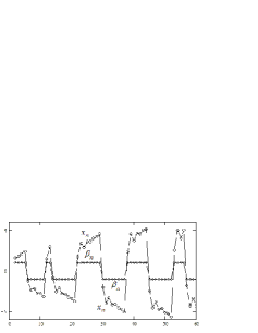
Figure 2: Oscillations in each solution $x_{n}$ exhibit the same pattern as those in the binary sequence $\beta_{n}$ generating it

The method of completing the square discussed in Example 8 can be applied to every quadratic difference equation with real coefficients. This useful feature enables the calculation of solutions of such quadratic equations through iteration, a feature that is not shared by non-recursive difference equations in general. The next result sets the stage by providing an essential ingredient for the existence theorem.

Lemma 9

In the quadratic difference equation

$$\sum_{i=0}^{k}\sum_{j=i}^{k}a_{i,j,n}x_{n-i}x_{n-j}+\sum_{j=0}^{k}b_{j,n}x_{n-j}+c_{n}=0$$ (44)

assume that all the coefficients $a_{i,j,n},b_{j,n},c_{n}$ are real numbers with $a_{0,0,n}\not=0$ for all $n.$ Then $\{x_{n}\}$ is a real solution of (44) if and only if $\{x_{n}\}$ is a real solution of some member of the family of recursive equations, namely, the recursive class of (44)

$$s_{n}=L_{n}(s_{n-1},\ldots,s_{n-k})+\beta_{n}\sqrt{L_{n}^{2}(s_{n-1},\ldots,s_{n-k})+Q_{n}(s_{n-1},\ldots,s_{n-k})}$$ (45)

where $\{\beta_{n}\}$ is a fixed but arbitrarily chosen binary sequence with values in the set $\{-1,1\}$ and for each $n,$

$$L_{n}(u_{1},\ldots,u_{k}) =\frac{-1}{2a_{0,0,n}}\left(b_{0,n}+\sum_{j=1}^{k}a_{0,j,n}u_{j}\right),$$ (46)

$$Q_{n}(u_{1},\ldots,u_{k}) =\frac{-1}{a_{0,0,n}}\left(\sum_{i=1}^{k}\sum_{j=i}^{k}a_{i,j,n}u_{i}u_{j}+\sum_{j=1}^{k}b_{j,n}u_{j}+c_{n}\right).$$ (47)

Proof. If

$$E_{n}(u_{0},u_{1},\ldots,u_{k})=\sum_{i=0}^{k}\sum_{j=i}^{k}a_{i,j,n}u_{i}u_{j}+\sum_{j=1}^{k}b_{j,n}u_{j}+c_{n}$$

then using definitions (46) and (47) we may write

$$E_{n}(u_{0},u_{1},\ldots,u_{k})=a_{0,0,n}[x_{n}^{2}-2L_{n}(u_{1},\ldots,u_{k})x_{n}-Q_{n}(u_{1},\ldots,u_{k})]$$ (48)

Since $a_{0,0,n}\not=0$ for all $n$, the solution set of (44) is identical to the solution set of

$$x_{n}^{2}-2L_{n}(u_{1},\ldots,u_{k})x_{n}-Q_{n}(u_{1},\ldots,u_{k})=0.$$ (49)

Completing the square in (49) gives

$$[x_{n}-L_{n}(u_{1},\ldots,u_{k})]^{2}=L_{n}^{2}(u_{1},\ldots,u_{k})+Q_{n}(u_{1},\ldots,u_{k}).$$

which is equivalent to (45).   

Example 8 provides a quick illustration of the preceding result with

$$L(u_{1},u_{2})=\frac{a}{2}u_{1},\quad Q(u_{1},u_{2})=bu_{2}^{2}+c$$

where $L_{n}=L$ and $Q_{n}=Q$ are independent of $n.$

We are now ready to present the existence theorem for real solutions of (44). Let $\{\beta_{n}\}$ be a fixed but arbitrarily chosen binary sequence in $\{-1,1\}$ and define the functions $L_{n}$ and $Q_{n}$ as in Lemma 9. Further, denote the functions on the right hand side of (45) by $f_{n},$ i.e.,

$$f_{n}(u_{1},\ldots,u_{k})=L_{n}(u_{1},\ldots,u_{k})+\beta_{n}\sqrt{L_{n}^{2}(u_{1},\ldots,u_{k})+Q_{n}(u_{1},\ldots,u_{k})}.$$ (50)

These functions on $\mathbb{R}^{k}$ unfold to the self-maps

$$F_{n}(u_{1},\ldots,u_{k})=\left(f_{n}(u_{1},\ldots,u_{k}),u_{1},\ldots,u_{k-1}\right).$$

We emphasize that each function sequence $\{F_{n}\}$ is determined by a given or fixed binary sequence $\{\beta_{n}\}$ as well as the function sequences $\{L_{n}\}$ and $\{Q_{n}\}$ that are given by (44). Clearly the functions $f_{n}$ are real-valued at a point $(u_{1},\ldots,u_{k})\in\mathbb{R}^{k}$ if and only if

$$L_{n}^{2}(u_{1},\ldots,u_{k})+Q_{n}(u_{1},\ldots,u_{k})\geq 0.$$ (51)

Theorem 10

Assume that the following set is nonemtpy:

$$\mathcal{S}={\displaystyle\bigcap\limits_{n=0}^{\infty}}\left\{(u_{1},\ldots,u_{k})\in\mathbb{R}^{k}:L_{n}^{2}(u_{1},\ldots,u_{k})+Q_{n}(u_{1},\ldots,u_{k})\geq 0\right\}.$$ (52)

(a) The quadratic difference equation (44) has a real solution $\{x_{n}\}_{n=-k+1}^{\infty}$ if and only if the point $P_{0}=(x_{0},x_{-1},\ldots,x_{-k+1})$ is in $\mathcal{S}$ and there is a binary sequence $\{\beta_{n}\}$ in $\{-1,1\}$ such that the forward orbit of $P_{0}$ under the associated maps $\{F_{n}\}$ is contained in $\mathcal{S};$ i.e.,

$$\{F_{n}\circ F_{n-1}\circ\cdots\circ F_{1}(P_{0})\}_{n=1}^{\infty}\subset\mathcal{S}.$$

(b) If the maps $\{F_{n}\}$ have a nonempty invariant set $M\subset\mathcal{S}$ for all $n,$ i.e.,

$$F_{n}(M)\subset M\subset\mathcal{S}$$

then the quadratic difference equation (44) has real solutions.

Proof. (a) By Lemma 9, $\{x_{n}\}_{n=-k+1}^{\infty}$ is a real solution of (44) if and only if there is a binary sequence $\{\beta_{n}\}$ in $\{-1,1\}$ such that $\{x_{n}\}_{n=-k+1}^{\infty}$ is a real solution of the recursive equation (45). Using the notation in (50), Eq.(45) can be written as

$$s_{n}=f_{n}(s_{n-1},\ldots,s_{n-k}).$$ (53)

Now the forward orbit of the solution $\{x_{n}\}_{n=-k+1}^{\infty}$ of (53) is the sequence

$$\mathcal{O}=\{F_{n}\circ F_{n-1}\circ\cdots\circ F_{1}(P_{0})\}_{n=1}^{\infty}=\{(x_{n-1},\ldots,x_{n-k})\}_{n=1}^{\infty}$$

in $\mathbb{R}^{k}$ that starts from $P_{0}\in\mathcal{S}.$ It is clear from the definition of $T$ that each $x_{n}$ is real if and only if $\mathcal{O}\subset\mathcal{S}.$ This observation completes the proof of (a).

(b) Let $P_{0}\in M.$ Then $\{F_{n}\circ F_{n-1}\circ\cdots\circ F_{1}(P_{0})\}_{n=1}^{\infty}\subset M\subset\mathcal{S}$ so by (a)

$$\{(x_{n-1},\ldots,x_{n-k})\}_{n=1}^{\infty}\subset\mathcal{S}.$$

It follows that each $x_{n}$ is real and thus, $\{x_{n}\}_{n=-k+1}^{\infty}$ of (53). An application of Lemma 9 now completes the proof.   

If $\mathcal{S}$ has any invariant subset $M=M(\{\beta_{n}\})$ (relative to some binary sequence $\{\beta_{n}\}$ in $\{-1,1\}$ or equivalently, to some map sequence $\{F_{n}\}$) then the union of all such invariant sets in $\mathcal{S}$ is again invariant relative to all relevant binary sequences $\{\beta_{n}\}$ (or map sequences $\{F_{n}\}$). Invariant sets may exist (i.e., they are nonempty) for some binary sequences $\{\beta_{n}\}$ in $\{-1,1\}$ and not others. However, the union of all invariant sets,

$$\mathcal{M}={\displaystyle\bigcup}\{M(\{\beta_{n}\}):\{\beta_{n}\}\text{ is a binary sequence in }\{-1,1\}\}$$

is the largest or maximal invariant set in $\mathcal{S}$ and as such, $\mathcal{M}$ is unique. In particular, if $\mathcal{S}$ is invariant relative to some binary sequence then $\mathcal{M=S}.$

We refer to $\mathcal{M}$ as the state-space of real solutions of (44). The existence of a (nonempty) $\mathcal{M}$ may signal the occurrence of a variety of solutions for (44). In Example 8, where $\mathcal{S}=\mathbb{R}^{2}$ is trivially invariant (so that $\mathcal{M=}\mathbb{R}^{2}$) we observed the occurrence of a wide variety of oscillatory behaviors. Generally, when $\mathcal{S}=\mathbb{R}^{k}$ every solution of (44) with its initial point $P_{0}\in\mathbb{R}^{k}$ is a real solution. The next result presents sufficient conditions that imply $\mathcal{S}=\mathbb{R}^{k}$. For cases where $\mathcal{S}$ is a proper subset of $\mathbb{R}^{k}$ see [10].

Corollary 11

The state-space of real solutions of (44) is $\mathbb{R}^{k}$ if the following conditions hold for all $n$:

$$A_{j,n} >0,\text{ }B_{i,j,n}=0,$$ (54)

$$\sum_{j=1}^{k}\frac{C_{j,n}^{2}}{A_{j,n}} \leq b_{0,n}^{2}-4a_{0,0,n}c_{n}$$ (55)

where for $k\geq 2$, $j=1,\ldots,k$, and $n\geq 0$

$$A_{j,n} =a_{0,j,n}^{2}-4a_{0,0,n}a_{j,j,n},$$

$$B_{i,j,n} =a_{0,i,n}a_{0,j,n}-2a_{0,0,n}a_{i,j,n},\ i<j,$$

$$C_{j,n} =a_{0,j,n}b_{0,n}-2a_{0,0,n}b_{j,n}.$$

Proof. By straightforward calculation the inequality $L_{n}^{2}+Q_{n}\geq 0,$ i.e., (51) is seen to be equivalent to

$$\sum_{j=1}^{k}A_{j,n}u_{j}^{2}+2\sum_{i=1}^{k-1}\sum_{j=i+1}^{k}B_{i,j,n}u_{i}u_{j}+2\sum_{j=1}^{k}C_{j,n}u_{j}+b_{0,n}^{2}\geq 4a_{0,0,n}c_{n}$$ (56)

for all $(u_{1},\ldots,u_{k})\in\mathbb{R}^{k}$ with the coefficients $A_{j,n}$, $B_{i,j,n}$ and $C_{j,n}$ as defined in the statement of the corollary. By conditions (55) the double summation term in (56) drops out and we may complete the squares in the remaining terms to obtain the inequality

$$\sum_{j=1}^{k}A_{j,n}\left(u_{j}+\frac{C_{j,n}}{A_{j,n}}\right)^{2}\geq\sum_{j=1}^{k}\frac{C_{j,n}^{2}}{A_{j,n}}-b_{0,n}^{2}+4a_{0,0,n}c_{n}.$$

By (54) the left hand side of the above inequality is non-negative while its right hand side is non-positive so (56) holds under conditions (54) and (55). The proof is completed by applying Theorem 10.   

The next result, which generalizes Example 8, is obtained by an immediate application of the above corollary to the non-homogeneous quadratic equation of order two with constant coefficients.

Corollary 12

The quadratic difference equation

$$x_{n}^{2}+a_{0,1}x_{n}x_{n-1}+a_{0,2}x_{n}x_{n-2}+a_{1,1}x_{n-1}^{2}+a_{1,2}x_{n-1}x_{n-2}+$$

$$\qquad\qquad+a_{2,2}x_{n-2}^{2}+b_{0}x_{n}+b_{1}x_{n-1}+b_{2}x_{n-2}+c_{n}=0$$

has $\mathbb{R}^{2}$ as a state-space of real solutions if the following conditions are satisfied:

$$a_{1,1} <\frac{a_{0,1}^{2}}{4},\quad a_{2,2}<\frac{a_{0,2}^{2}}{4},\quad a_{1,2}=\frac{1}{2}a_{0,1}a_{0,2}\text{ and}$$

$$c_{n} \leq\frac{b_{0}^{2}}{4}-\frac{(a_{0,1}b_{0}-2b_{1})^{2}}{4(a_{0,1}^{2}-4a_{1,1})}-\frac{(a_{0,2}b_{0}-2b_{2})^{2}}{4(a_{0,2}^{2}-4a_{2,2})}\text{ for all }n.$$

3.2 Factorization of quadratic equations

In the remainder of this paper we investigate conditions for the possible existence of a special semi-invertible form symmetry for quadratic difference equations in which both $\mu_{n}$ and $\theta_{n}$ are linear maps on $\mathcal{F}$ for all $n$; hence, this is called a linear form symmetry. This is a first step in a broader study of the latter type of equation on algebraic fields; see [10] for further discussion.

To simplify the discussion without losing sight of essential ideas, we limit attention to the case $k=2,$ i.e., the second-order equation

$$E_{n}(x_{n},x_{n-1},x_{n-2})=0$$ (57)

on a field $\mathcal{F}$ where

$$E_{n}(u_{0},u_{1},u_{2}) =a_{0,0,n}u_{0}^{2}+a_{0,1,n}u_{0}u_{1}+a_{0,2,n}u_{0}u_{2}+$$ (58)

$$\quad a_{1,0,n}u_{1}^{2}+a_{1,2,n}u_{1}u_{2}+a_{2,0,n}u_{2}^{2}+$$

$$\qquad b_{0,n}u_{0}+b_{1,n}u_{1}+b_{2,n}u_{2}+c_{n}.$$

In this expression, to assure that $u_{0}$ (corresponding to the $x_{n}$ term) does not drop out, we may assume that for each $n,$

$$\text{if }a_{0,0,n}=a_{0,1,n}=b_{0,n}=0\text{ or }a_{1,2,n}=a_{2,0,n}=b_{2,n}=0,\text{ then }a_{0,2,n}\not=0.$$

If the quadratic expression (58) has a form symmetry $\{H_{n}\}$ where

$$H_{n}(u_{0},u_{1},u_{2})=[h_{n}(u_{0},u_{1}),h_{n-1}(u_{1},u_{2})]$$

then there are sequences $\{\phi_{n}\},\{h_{n}\}$ of functions $\phi_{n},h_{n}:\mathcal{F}^{2}\rightarrow\mathcal{F}$ such that for all $(u_{0},u_{1},u_{2})\in\mathcal{F}^{3},$

$$\phi_{n}(h_{n}(u_{0},u_{1}),h_{n-1}(u_{1},u_{2}))=E_{n}(u_{0},u_{1},u_{2}).$$ (59)

The form symmetry $\{H_{n}\}$ is semi-invertible if there are bijection $\mu_{n},\theta_{n}:\mathcal{F}\rightarrow\mathcal{F}$ such that

$$h_{n}(u,v)=\mu_{n}(u)+\theta_{n}(v).$$

The next corollary of Theorem 5 presents conditions that imply the existence of a linear form symmetry for Eq.(57).

Corollary 13

The quadratic difference equation (57) has the linear form symmetry

$$h_{n}(u,v)=\alpha_{n}u+v,\quad\alpha_{n}\not=0\text{ for all }n$$ (60)

if and only if a sequence $\{\alpha_{n}\}$ exists in the field $\mathcal{F}$ such that all four of the following first-order equations are satisfied:

$$a_{0,0,n}-a_{0,1,n}\alpha_{n}+a_{1,1,n}\alpha_{n}^{2}+a_{0,2,n}\alpha_{n}\alpha_{n-1}-a_{1,2,n}\alpha_{n}^{2}\alpha_{n-1}+a_{2,2,n}\alpha_{n}^{2}\alpha_{n-1}^{2} =0$$ (61)

$$a_{0,1,n}-2a_{1,1,n}\alpha_{n}-a_{0,2,n}\alpha_{n-1}+2a_{1,2,n}\alpha_{n}\alpha_{n-1}-2a_{2,2,n}\alpha_{n}\alpha_{n-1}^{2} =0$$ (62)

$$a_{0,2,n}-a_{1,2,n}\alpha_{n}+2a_{2,2,n}\alpha_{n}\alpha_{n-1} =0$$ (63)

$$b_{0,n}-b_{1,n}\alpha_{n}+b_{2,n}\alpha_{n}\alpha_{n-1} =0.$$ (64)

In this case, Eq.(57) has a factorization with a first-order factor equation

$$(a_{1,1,n}-a_{1,2,n}\alpha_{n-1}+a_{2,2,n}\alpha_{n-1}^{2})t_{n}^{2}+a_{2,2,n}t_{n-1}^{2}+(a_{1,2,n}-2a_{2,2,n}\alpha_{n-1})t_{n}t_{n-1}$$

$$+(b_{1,n}-b_{2,n}\alpha_{n-1})t_{n}+b_{2,n}t_{n-1}+c_{n}=0.$$

and a cofactor equation $\alpha_{n}x_{n}+x_{n-1}=t_{n}$ also of order one.

Proof. For any nonzero sequence $\{\alpha_{n}\}$ in $\mathcal{F}$ the functions $h_{n}$ defined by (60) are semi-invertible with $\mu_{n}(u)=\alpha_{n}u$ and $\theta_{n}(v)=v$ for all $n.$ Note that $\theta_{n}^{-1}=\theta_{n}$ for all $n$ and the group structure is the additive group of the field so the quantities $\zeta_{j,n}$ in Theorem 5 take the forms

$$\zeta_{1,n} =\zeta_{1,n}(u_{0},v_{1})=-\alpha_{n}u_{0}+v_{1},$$

$$\zeta_{2,n} =\zeta_{2,n}(u_{0},v_{1},v_{2})=\alpha_{n}\alpha_{n-1}u_{0}-\alpha_{n-1}v_{1}+v_{2}.$$

By Theorem 5, Eq.(57) has the linear form symmetry if and only if the expression $E_{n}=E_{n}(u_{0},\zeta_{1,n},\zeta_{2,n})$ is independent of $u_{0}$ for all $n.$ Now

$$E_{n} =a_{0,0,n}u_{0}^{2}+a_{0,1,n}u_{0}(v_{1}-\alpha_{n}u_{0})+$$

$$a_{0,2,n}u_{0}(\alpha_{n}\alpha_{n-1}u_{0}-\alpha_{n-1}v_{1}+v_{2})+a_{1,1,n}(v_{1}-\alpha_{n}u_{0})^{2}+$$

$$a_{1,2,n}(v_{1}-\alpha_{n}u_{0})(\alpha_{n}\alpha_{n-1}u_{0}-\alpha_{n-1}v_{1}+v_{2})+$$

$$a_{2,2,n}(\alpha_{n}\alpha_{n-1}u_{0}-\alpha_{n-1}v_{1}+v_{2})^{2}+b_{0,n}u_{0}+$$

$$b_{1,n}(v_{1}-\alpha_{n}u_{0})+b_{2,n}(\alpha_{n}\alpha_{n-1}u_{0}-\alpha_{n-1}v_{1}+v_{2})+c_{n}.$$

Multiplying terms in the above expression gives

$$E_{n} =a_{0,0,n}u_{0}^{2}+a_{0,1,n}u_{0}v_{1}-a_{0,1,n}\alpha_{n}u_{0}^{2}+a_{0,2,n}\alpha_{n}\alpha_{n-1}u_{0}^{2}-$$

$$a_{0,2,n}\alpha_{n-1}u_{0}v_{1}+a_{0,2,n}u_{0}v_{2}+a_{1,1,n}v_{1}^{2}-2a_{1,1,n}\alpha_{n}u_{0}v_{1}+$$

$$a_{1,1,n}\alpha_{n}^{2}u_{0}^{2}+a_{1,2,n}\alpha_{n}\alpha_{n-1}u_{0}v_{1}-a_{1,2,n}\alpha_{n-1}v_{1}^{2}+a_{1,2,n}v_{1}v_{2}-$$

$$a_{1,2,n}\alpha_{n}^{2}\alpha_{n-1}u_{0}^{2}+a_{1,2,n}\alpha_{n}\alpha_{n-1}u_{0}v_{1}-a_{1,2,n}\alpha_{n}u_{0}v_{2}+$$

$$a_{2,2,n}\alpha_{n}^{2}\alpha_{n-1}^{2}u_{0}^{2}-2a_{2,2,n}\alpha_{n}\alpha_{n-1}^{2}u_{0}v_{1}+2a_{2,2,n}\alpha_{n}\alpha_{n-1}u_{0}v_{2}+$$

$$a_{2,2,n}(\alpha_{n-1}v_{1}-v_{2})^{2}+b_{0,n}u_{0}+b_{1,n}v_{1}-b_{1,n}\alpha_{n}u_{0}+$$

$$b_{2,n}\alpha_{n}\alpha_{n-1}u_{0}-b_{2,n}(\alpha_{n-1}v_{1}-v_{2})+c_{n}.$$

Terms containing $u_{0}$ or $u_{0}^{2}$ must sum to zeros. Rearranging terms in the preceding expression gives

$$E_{n} =(a_{0,0,n}-a_{0,1,n}\alpha_{n}+a_{0,2,n}\alpha_{n}\alpha_{n-1}+a_{1,1,n}\alpha_{n}^{2}-a_{1,2,n}\alpha_{n}^{2}\alpha_{n-1}+$$

$$a_{2,2,n}\alpha_{n}^{2}\alpha_{n-1}^{2})u_{0}^{2}+(a_{0,1,n}-a_{0,2,n}\alpha_{n-1}-2a_{1,1,n}\alpha_{n}+$$

$$2a_{1,2,n}\alpha_{n}\alpha_{n-1}-2a_{2,2,n}\alpha_{n}\alpha_{n-1}^{2})u_{0}v_{1}+(a_{0,2,n}-a_{1,2,n}\alpha_{n}+$$

$$2a_{2,2,n}\alpha_{n}\alpha_{n-1})u_{0}v_{2}+(b_{0,n}-b_{1,n}\alpha_{n}+b_{2,n}\alpha_{n}\alpha_{n-1})u_{0}+$$

$$(a_{1,1,n}-a_{1,2,n}\alpha_{n-1}+a_{2,2,n}\alpha_{n-1}^{2})v_{1}^{2}+a_{2,2,n}v_{2}^{2}+(a_{1,2,n}-$$

$$2a_{2,2,n}\alpha_{n-1})v_{1}v_{2}+(b_{1,n}-b_{2,n}\alpha_{n-1})v_{1}+b_{2,n}v_{2}+c_{n}.$$

Setting the coefficients of variable terms containing $u_{0}$ equal to zeros gives the four first-order equations (61)-(64). The part of $E_{n}$ above that does not vanish yields the factor functions

$$\phi_{n}(v_{1},v_{2}) =(a_{1,1,n}-a_{1,2,n}\alpha_{n-1}+a_{2,2,n}\alpha_{n-1}^{2})v_{1}^{2}+a_{2,2,n}v_{2}^{2}+$$

$$\qquad(a_{1,2,n}-2a_{2,2,n}\alpha_{n-1})v_{1}v_{2}+(b_{1,n}-b_{2,n}\alpha_{n-1})v_{1}+b_{2,n}v_{2}+c_{n}.$$

This expression plus the linear cofactor $t_{n}=h_{n}(x_{n},x_{n-1})=\alpha_{n}x_{n}+x_{n-1}$ give the stated factorization.   

An immediate consequence of Corollary 13 is that every second-order, non-homogeneous linear difference equation

$$x_{n}+b_{1,n}x_{n-1}+b_{2,n}x_{n-2}+c_{n}=0$$

has a linear form symmetry and the corresponding factorization into a pair of equations of order one (also non-homogeneous, linear) if and only if the first-order difference equation (64) has a solution $\{\alpha_{n}\}$ in $\mathcal{F}\backslash\{0\}$. The existence of a linear form symmetry for non-homogeneous linear equations of all orders can be established by a calculation similar to that in the proof of Corollary 13. However, as noted earlier, a complete proof for the general case is already given in [12] using the semiconjugate factorization method which applies to linear equations because they are recursive. Therefore, we need not consider the linear case any further here.

If all coefficients in $E_{n}(u_{0},u_{1},u_{2})$ are constants except possibly the free term $c_{n}$ then a simpler version of Corollary 13 is obtained as follows.

Corollary 14

The quadratic difference equation with constant coefficients

$$a_{0,0}x_{n}^{2}+a_{0,1}x_{n}x_{n-1}+a_{0,2}x_{n}x_{n-2}+a_{1,1}x_{n-1}^{2}+a_{1,2}x_{n-1}x_{n-2}$$

$$+a_{2,2}x_{n-2}^{2}+b_{0}x_{n}+b_{1}x_{n-1}+b_{2}x_{n-2}+c_{n}=0$$ (65)

in a non-trivial field $\mathcal{F}$ has the linear form symmetry with $h(u,v)=\alpha u+v$ if and only if the following polynomials have a common nonzero root $\alpha$ in $\mathcal{F}$:

$$a_{0,0}-a_{0,1}\alpha+(a_{1,1}+a_{0,2})\alpha^{2}-a_{1,2}\alpha^{3}+a_{2,2}\alpha^{4} =0,$$ (66)

$$a_{0,1}-(a_{0,2}+2a_{1,1})\alpha+2a_{1,2}\alpha^{2}-2a_{2,2}\alpha^{3} =0,$$ (67)

$$a_{0,2}-a_{1,2}\alpha+2a_{2,2}\alpha^{2} =0,$$ (68)

$$b_{0}-b_{1}\alpha+b_{2}\alpha^{2} =0.$$ (69)

If such a root $\alpha\not=0$ exists then Eq.(65) has the factorization

$$(a_{1,1}-a_{1,2}\alpha+a_{2,2}\alpha^{2})t_{n}^{2}+(a_{1,2}-2a_{2,2}\alpha)t_{n}t_{n-1}+a_{2,2}t_{n-1}^{2}$$

$$+(b_{1}-b_{2}\alpha)t_{n}+b_{2}t_{n-1}+c_{n}=0,$$

$$x_{n}=-\frac{1}{\alpha}x_{n-1}+\frac{t_{n}}{\alpha}.$$

Equalities (66)-(69) often lead to suitable parameter restrictions implying the existence of a linear form symmetry for a given difference equation. Here is a sample.

Example 15

Consider the following quadratic equation (no linear terms)

$$x_{n}^{2}+ax_{n}x_{n-1}+bx_{n}x_{n-2}+cx_{n-1}x_{n-2}=\sigma_{n}.$$ (70)

In the absence of linear terms in (70) equality (69) holds trivially; the other three equalities (66)-(68) take the following forms

$$1-a\alpha+b\alpha^{2}-c\alpha^{3} =0$$ (71)

$$a-b\alpha+2c\alpha^{2} =0$$ (72)

$$b-c\alpha =0.$$ (73)

From (73) it follows that $\alpha=b/c.$ This nonzero value of $\alpha$ must satisfy the other two equations in the above system so from (72) we obtain

$$a+\frac{b^{2}}{c}=0$$

while (71) yields

$$1-\frac{ab}{c}=0\quad\text{or\quad}c=ab.$$

Eliminating $b$ and $c$ from the last two equations gives

$$b=-a^{2},\ c=-a^{3}\ \text{and }\alpha=\frac{1}{a}.$$

These calculations indicate that the quadratic equation

$$x_{n}^{2}+ax_{n}x_{n-1}-a^{2}x_{n}x_{n-2}-a^{3}x_{n-1}x_{n-2}=\sigma_{n}$$

has the linear form symmetry with the corresponding factorization

$$a^{2}t_{n}^{2}-a^{3}t_{n}t_{n-1} =\sigma_{n},$$

$$x_{n}+ax_{n-1} =at_{n}.$$

Corollary 14 also implies the non-existence of a linear form symmetry. The next example illustrates this fact.

Example 16

Let $a,b\in\mathbb{C}$ with $b\not=0$ and let $\{c_{n}\}$ be a sequence of complex numbers. Then the difference equation

$$x_{n}^{2}+ax_{n-1}^{2}+bx_{n-2}^{2}=c_{n}$$ (74)

does not have a linear form symmetry because the equality (68) in Corollary 14 does not hold for a nonzero complex number $\alpha.$ On the other hand, the substitution $y_{n}=x_{n}^{2}$ transforms (74) into the non-homogeneous linear equation

$$y_{n}+ay_{n-1}+by_{n-2}=c_{n}$$

which does have a linear form symmetry in $\mathbb{C}$ (by Corollary 14, with equality (69) implying that $-\alpha$ is an eigenvalue of the homogeneous part). Substituting $x_{n}^{2}$ for $y_{n}$ in the resulting cofactor equation gives a factorization of (74).

References

• [1] Bertram, W., “Difference problems and differential problems”, in Contemp. Geom. Topol. and Related Topics, Proceedings of Eighth Int. Workshop on Differential Geometry and its Applications, Cluj-Napoca, 73-87, 2007
• [2] Camouzis, E. and Ladas, G., Dynamics of Third Order Rational Difference Equations with Open Problems and Conjectures, Chapman and Hall/CRC Press, Boca Raton, 2008
• [3] Dehghan, M., Mazrooei-Sebdani, R. and Sedaghat, H., Global behavior of the Riccati difference equation of order two, J. Difference Eqs. and Appl., to appear.
• [4] Dehghan, M., Kent, C.M., Mazrooei-Sebdani, R., Ortiz, N.L. and Sedaghat, H., Monotone and oscillatory solutions of a rational difference equation containing quadratic terms, J. Difference Eqs. and Appl., 14 (2008) 1045-1058.
• [5] Dehghan, M., Kent, C.M., Mazrooei-Sebdani, R., Ortiz, N.L. and Sedaghat, H., Dynamics of rational difference equations containing quadratic terms, J. Difference Eqs. and Appl., 14 (2008) 191-208.
• [6] Grove, E.A. and Ladas, G., Periodicities in Nonlinear Difference Equations, CRC Press, Boca Raton, 2005
• [7] Kent, C.M. and Sedaghat, H., Convergence, periodicity and bifurcations for the two-parameter absolute difference equation, J. Difference Eqs. and Appl., 10 (2004) 817-841.
• [8] Kocic, V.L. and Ladas, G., Global Behavior of Nonlinear Difference Equations of Higher Order with Applications, Kluwer, Dordrecht, 1993
• [9] Kulenovic, M.R.S. and Ladas, G., Dynamics of Second Order Rational Difference Equations with Open Problems and Conjectures, Chapman and Hall/CRC, Boca Raton, 2002
• [10] Sedaghat, H., Form Symmetries and Reduction of Order in Difference Equations (forthcoming) CRC Press, Boca Raton, 2011.
• [11] Sedaghat, H., Reductions of order in difference equations defined as products of exponential and power functions, J. Difference Eqs. and Appl., to appear.
• [12] Sedaghat, H., Factorization of difference equations by semiconjugacy with application to non-autonomous linear equations (2010) http://arxiv.org/abs/1005.2428
• [13] Sedaghat, H., Semiconjugate factorization of non-autonomous higher order difference equations, Int. J. Pure and Appl. Math., 62 (2010) 233-245.
• [14] Sedaghat, H., Every homogeneous difference equation of degree one admits a reduction in order, J. Difference Eqs. and Appl., 15 (2009) 621-624.
• [15] Sedaghat, H., Reduction of order in difference equations by semiconjugate factorizations, Int. J. Pure and Appl. Math., 53 (2009) 377-384.
• [16] Sedaghat, H., Global behaviors of rational difference equations of orders two and three with quadratic terms, J. Difference Eqs. and Appl., 15 (2009) 215-224.
• [17] Sedaghat, H., Periodic and chaotic behavior in a class of second order difference equations, Adv. Stud. Pure Math., 53 (2009) 321-328.
• [18] Sedaghat, H., Semiconjugate factorization and reduction of order in difference equations (2009) http://arxiv.org/abs/0907.3951
• [19] Sedaghat, H., Nonlinear Difference Equations: Theory with Applications to Social Science Models, Kluwer, Dordrecht, 2003.
• [20] Smital, J., Why it is important to understand the dynamics of triangular maps”, J. Difference Eqs. and Appl., 14 (2008) 597-606.