Virial Theorem and Hypervirial Theorem in a spherical geometry

Abstract

The Virial Theorem in the one- and two-dimensional spherical geometry are presented, in both classical and quantum mechanics. Choosing a special class of Hypervirial operators, the quantum Hypervirial relations in the spherical spaces are obtained. With the aid of the Hellmann-Feynman Theorem, these relations can be used to formulate a perturbation theorem without wave functions, corresponding to the Hypervirial-Hellmann-Feynman Theorem perturbation theorem of Euclidean geometry. The one-dimensional harmonic oscillator and two-dimensional Coulomb system in the spherical spaces are given as two sample examples to illustrate the perturbation method.

1 Introduction

The Virial Theorem (VT) has been known for a long time in both classical mechanics and quantum mechanics. In the classical case, it provides a general equation relating the average over time of the kinetic energy $\langle T\rangle$ with that of the function of potential energy $\langle\vec{r}\cdot\nabla V\rangle$. The VT was given its technical definition by Clausius in 1870 [1]. Mathematically, the theorem states

$$2\langle T\rangle=\langle\vec{r}\cdot\nabla V\rangle.$$ (1)

If the potential takes the power function $V(r)=\alpha r^{n}$ with $r=|\vec{r}|$, the VT adopts a simple form as

$$2\langle T\rangle=n\langle V\rangle.$$ (2)

Thus, twice the average kinetic energy equals $n$ times the average potential energy. The VT in quantum mechanics has the same form as the classical one, except for the average over time in Eqs. (1) and (2) replacing by the average over an energy eigenstate of the system. It dates back to the old papers of Born, Heisenberg and Jordan [2], and is derived from the fact that the expectation value of the time-independent operator $\vec{r}\cdot\vec{p}$ under a eigenstate is a constant [3],

$$i\frac{d}{dt}\langle\psi|\vec{r}\cdot\vec{p}|\psi\rangle=\langle\psi|[\vec{r}\cdot\vec{p},H]|\psi\rangle=0,$$ (3)

where $H=\frac{p^{2}}{2}+V$ is the Hamiltonian and $|\psi\rangle$ is an eigenket of $H$.

In 1960, Hirschfelder [4] generalized the relationship by pointing out that $\vec{r}\cdot\vec{p}$ could be replaced by any other operators which were not dependent on time explicitly. In this way, he established the Hypervirial Theorem (HVT). For example, in a one-dimensional system, one can replace $\vec{r}\cdot\vec{p}=xp$ by the hypervirial operator $x^{k}p$, and obtain the recurrence relation of $\langle x^{k}\rangle$,

$$2kE\langle x^{k-1}\rangle=2k\langle x^{k-1}V\rangle+\langle x^{k}\frac{dV}{dx}\rangle-\frac{1}{4}k(k-1)(k-2)\langle x^{k-3}\rangle,$$ (4)

where $k$ is an integer and $E$ is the eigenenergy.

The Hellmann-Feynman (HF) Theorem is another important theorem in quantum mechanics, which has been applied to the force concept in molecules by using the internuclear distance as a parameter [5, 6]. Let the Hamiltonian $H(\xi)$ of a system be a time-independent operator that depends explicitly upon a continuous parameter $\xi$, and $|\psi(\xi)\rangle$ be a normalized eigenfunction of $H(\xi)$ with the eigenvalue $E_{m}(\xi)$, i.e. $H(\xi)|\psi(\xi)\rangle=E_{m}(\xi)|\psi(\xi)\rangle$, $\langle\psi(\xi)|\psi(\xi)\rangle=1$. The HF theorem states that

$$\frac{\partial E_{m}(\xi)}{\partial\xi}=\langle\psi(\xi)|\frac{\partial H(\xi)}{\partial\xi}|\psi(\xi)\rangle.$$ (5)

If the potential takes the power function $V(r)=\alpha r^{n}$, the HF gives an equation representing the relation between eigenenergy $E_{m}$ and mean value of $r^{n}$,

$$\frac{\partial E_{m}}{\partial\alpha}=\langle r^{n}\rangle.$$ (6)

Based on the relations in Eqs. (4) and (6), the Hypervirial-Hellmann-Feynman Theorem (HVHF) perturbation theorem is established [7, 8]. It provides a very efficient algorithm for the generation of perturbation expansions to large order, replacing the formal manipulation of Fourier series expansions with recursion relations. This perturbation method just need the energy instead of the wave functions of the system, and it is easy to achieve on the computer.

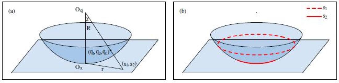
Figure 1: (a) The gnomonic projection, which is the projection onto the tangent plane from the center of the sphere in the embedding space. (b) Two classical orbits are shown as $s_{1}$ (dashed line) and $s_{2}$ (solid line), corresponding to the circular motion and the radial one respectively.

These results are well known, but have not, to our knowledge, been exploited in a curved space. In the present work, we focus on the one- and two-dimensional spherical geometry. The coordinate systems adopted in this paper are shown in Fig. 1 (a): (i) An intuitive way to describe a two-dimensional sphere is to embed it in a three-dimensional Euclidean space. Each pair of independent variables $(q_{1},q_{2})$ of the three-dimensional Cartesian coordinates $(q_{1},q_{2},q_{0})$, with the origin $O_{q}$ in the figure, under the constraint

$$q_{0}^{1}+q_{1}^{2}+q_{2}^{2}=\frac{1}{\lambda}$$ (7)

corresponds to two points of the sphere, where $\lambda$ is the curvature of the sphere. The points on the sphere can also be described by the spherical polar coordinate $(R,\chi,\theta)$ defined by $(q_{1},q_{2},q_{0})=(R\sin\chi\cos\theta,R\sin\chi\sin\theta,R\cos\chi)$ with $R=1/\sqrt{\lambda}$ being a constant. (ii) The Cartesian coordinates $(x_{1},x_{2})$ of the two-dimensional gnomonic projection, which is the projection onto the tangent plane from the center of the sphere in the embedding space, is given by

$$q_{1}=\frac{x_{1}}{\sqrt{1+\lambda r^{2}}},\ \ \ \ \ \ \ \ \ q_{2}=\frac{x_{2}}{\sqrt{1+\lambda r^{2}}}$$ (8)

where $r^{2}=x_{1}^{2}+x_{2}^{2}$ and the point of tangency $O_{x}$ in the figure being the origin. And the polar coordinate $(r,\theta)$ of the projection is defined by $r=R\tan\chi$ and $(x_{1},x_{2})=(r\cos\theta,r\sin\theta)$. In this work, we mainly adopt the two coordinate systems, $(x_{1},x_{2})$ and $(r,\theta)$, considering the results of Higgs [9] introduced in the following.

In 1979, Higgs [9] introduced a generalization of the hydrogen atom and harmonic oscillator in a spherical space. He demonstrated that, in the gnomonic projection as shown in Fig. 1 (a), the orbits of the motion on a sphere can be described by

$$\frac{1}{2}L^{2}[r^{-4}(\frac{dr}{d\theta})^{2}+r^{-2}]+V(r)=E-\frac{1}{2}\lambda L^{2},$$ (9)

where the angular momentum $L=x_{1}p_{2}-x_{2}p_{1}$ is an invariant quantity with the potential $V(r)$ being radial symmetric The Hamiltonian can be written as

$$H=\frac{\pi^{2}}{2}+\frac{1}{2}\lambda L^{2}+V(r),$$ (10)

where $\vec{\pi}=\vec{p}+\frac{\lambda}{2}\left[\vec{x}(\vec{x}\cdot\vec{p})+(\vec{p}\cdot\vec{x})\vec{x}\right]$ is the conserved vector in free particle motion on the sphere. Since the curvature appears only in the right combination $E-\frac{1}{2}\lambda L^{2}$ of Eq. (9), the projected orbits are the same, for a given $V(r)$, as in Euclidean geometry. Consequently, according with the Bertrand Theorem [10, 11], the orbits are closed only if the potential takes the Coulomb or isotropic oscillator form, i.e. $V(r)=-\frac{\kappa}{r}$ or $V(r)=\frac{1}{2}\omega^{2}r^{2}$, with $\kappa$ and $\omega$ being constants. Therefore the systems described by Eq. (10) with the two mentioned potentials are defined as the Kepler problem and isotropic oscillator in a spherical geometry in [9]. The algebraic relations of their conserved quantities reveal the dynamical symmetries of the two systems are described by the $SO(3)$ and $SU(2)$ Lie groups respectively. These results are the beginning of the so called Higgs Algebra, which has been studied in a variety of directions [12, 13, 14, 15, 16].

The concept of symmetry is one of the cornerstones in the modern physic, and dynamical symmetry plays a important role in many important physical models. Since the dynamical symmetries of the Kepler problem and isotropic oscillator on a $2$-sphere described by Eq. (10) adhere to the behaviors in two-dimensional Euclidean geometry, our question is: Do there exist more qualities of being homogeneous? This paper is aimed at constructing the VT and the HVT for the spherical geometry and studying their applications. In this work, we focus on the two- and one-demential cases for simplicity. On the other hand, the motion on of a charged particle on a $2$-sphere is not trivial, which is related with the famous fractionally quantized Hall states [17, 18]. We provide a general equation relating the average of the kinetic energy with that of the potential energy in the spherical geometry. We also give a generalized HVHF, which could propose to solve a class of problems the sense of perturbation.

The article is organized as follows: In the Sec. 2, the VT in both classical mechanics and quantum mechanics is constructed. In the Sec. 3, we generalize the VT to HVT, and give the quantum hypervirial relation. Two examples are taken to demonstrate the perturbation method which is combined HVT with HF theorem in the Sec. 4. We end this paper with some relevant discussions in the last section.

2 Virial Theorem

2.1 Classical Mechanics

To obtain the classical VT in the two-dimensional spherical geometry, two we special orbits are listed in the following for examples. (i) The first one is the uniform circular motion with $\dot{r}=0$ as shown by the curve $s_{1}$ in Fig. 1 (a). The kinetic energy of this case is given by

$$T=\frac{1}{2}(R\sin\chi_{0})^{2}\dot{\theta}^{2},$$

where $R\sin\chi_{0}$ is the radius of the path. The corresponding centripetal force is

$$F=\frac{2T}{R\sin\chi_{0}}=\frac{(1+\lambda r^{2})\vec{r}\cdot\nabla V}{R\sin\chi_{0}}.$$ (11)

Hence, one can obtain

$$2\langle T\rangle=\langle(1+\lambda r^{2})\vec{r}\cdot\nabla V\rangle,$$ (12)

which can be considered as the VT under the case of uniform circular motion. (ii) The orbit $s_{2}$ in Fig. 1 (b) depictes the case which the angular momentum $L$ is zero. In the same way, the relationship between kinetic energy and potential energy can be obtain as

$$2\langle(1+\lambda r^{2})T\rangle=\langle(1+\lambda r^{2})\vec{r}\cdot\nabla V\rangle.$$ (13)

These serve a good inspiration for us to presume that the VT in a spherical geometry is

$$2\langle(1+\lambda r^{2})T_{r}\rangle+2\langle T_{\theta}\rangle=\langle(1+\lambda r^{2})\vec{r}\cdot\nabla V\rangle,$$ (14)

where $T_{r}$ and $T_{\theta}$ are the radial and rotational kinetic energy.

In A, we give a proof that Eq. (14) is satisfied for an arbitrary orbit in the spherical space, and it equivalents to

$$\langle(1+\lambda r^{2})\vec{r}\cdot\nabla V\rangle=\langle(1+\lambda r^{2})\pi^{2}\rangle=\langle(1+\lambda r^{2})(2T-\lambda L^{2})\rangle.$$ (15)

where $L=x_{1}p_{2}-x_{2}p_{1}$ is the angular momentum. It is easy to find that, when the curvature $\lambda\rightarrow 0$, the above result reduces to Eq. (1).

2.2 Quantum Mechanics

In the literature [9], to construct the the conserved quantities on the sphere, Higgs replaced the momentum $\vec{p}$ in the generators on the plan by the vector $\vec{\pi}$. This enlightens us on the subject that we can replace $\vec{r}\cdot\vec{p}$ in Eq.(3) by $\vec{r}\cdot\vec{\pi}+\vec{\pi}\cdot\vec{r}$ to obtain the VT on the sphere. The expected value of the commutator is

$$\langle[\vec{r}\cdot\vec{\pi}+\vec{\pi}\cdot\vec{r},H]\rangle=0.$$ (16)

For the system in the one-dimensional curve, whose Hamiltonian is given by $H=\pi^{2}/2+V$ with $\pi=p+\lambda(x^{2}p+px^{2})/2$, the above relation leads to

$$\langle(1+\lambda x^{2})\frac{\pi^{2}}{2}+\frac{\pi^{2}}{2}(1+\lambda x^{2})\rangle+\frac{1}{2}\langle\lambda(1+\lambda x^{2})(1+3\lambda x^{2})\rangle=\langle(1+\lambda x^{2})x\frac{dV}{dx}\rangle.$$ (17)

And in the two-dimensional case, from Eq.(10) and Eq.(16), we obtain

$$\langle(1+\lambda r^{2})\frac{\pi^{2}}{2}+\frac{\pi^{2}}{2}(1+\lambda r^{2})\rangle+\frac{1}{2}\langle\lambda(1+\lambda r^{2})(2+3\lambda r^{2})\rangle=\langle(1+\lambda r^{2})\vec{r}\cdot\nabla V\rangle.$$ (18)

In the polar coordinate, the Hamiltonian (10) can be written as

$$H_{0}=T_{r}+T_{\theta}+V,$$

$$T_{r}=-\frac{1}{2}\biggr{[}3\lambda+\frac{15}{4}\lambda^{2}r^{2}+\frac{(1+\lambda r^{2})(1+5\lambda r^{2})}{r}\frac{\partial}{\partial r}+(1+\lambda r^{2})^{2}\frac{\partial^{2}}{\partial r^{2}}\biggr{]},$$ (19)

$$T_{\theta}=-\frac{1}{2}\biggr{[}\frac{1}{r^{2}}\frac{\partial^{2}}{\partial\theta^{2}}+\lambda\frac{\partial^{2}}{\partial\theta^{2}}\biggr{]},$$

where $T_{r}$ and $T_{\theta}$ denote the radial and rotational kinetic energy. The relation of Eq. (18) equivalents to

$$\langle(1+\lambda r^{2})T_{r}+T_{r}(1+\lambda r^{2})\rangle+2\langle T_{\theta}\rangle+\frac{1}{2}\langle\lambda(1+\lambda r^{2})(2+3\lambda r^{2})\rangle=\langle(1+\lambda r^{2})\vec{r}\cdot\nabla V\rangle.$$ (20)

These results have the same form with the classical mechanical counterparts in Eqs. (14) and (15), but with a term $\frac{1}{2}\langle\lambda(1+\lambda r^{2})(2+3\lambda r^{2})\rangle$ in addition. And, the term is different from the corresponding one in the one-dimensional case (17), which comes from the commutation relation of $\vec{r}$ and $\vec{\pi}$.

3 Hypervirial Theorems

In the above, we have got the VT in both classical mechanics and quantum mechanics. We will discuss the quantum HVT in the present part. A natural candidate of the hypervirial operator is $r^{k}\pi+\pi r^{k}$ according to $r^{k}p$ in the plane we mentioned in Sec. 1, with $k$ being integers.

3.1 One-dimensional

In the one-dimensional case, one can calculate directly the commutation relation in the expected value

$$\langle[x^{k}\pi+\pi x^{k},H]\rangle=0,$$ (21)

and obtain

$$[x^{k}\pi+\pi x^{k},H] = i\frac{k}{2}\biggr{\{}2(1+\lambda x^{2})x^{k-1}\pi^{2}+2\pi^{2}(1+\lambda x^{2})x^{k-1}$$ (22)

$$+(1+\lambda x^{2})\bigr{[}(k-1)(k-2)x^{k-3}+2\lambda k^{2}x^{k-1}+\lambda^{2}(k+1)(k+2)x^{k+1}\bigr{]}\biggr{\}}$$

$$-2ix^{k}(1+\lambda x^{2})\frac{dV}{dx}.$$

Because of $\pi^{2}/2=H-V$ and $\langle H\rangle=E_{n}$ being the eigenvalues of the eigenstate, the Eq. (21) turns to

$$2kE_{n}\langle x^{k-1}\rangle_{\lambda}-2k\langle x^{k-1}V\rangle_{\lambda}-\langle x^{k}\frac{dV}{dx}\rangle_{\lambda}$$

$$+\frac{k}{4}\bigr{[}(k+1)(k+2)\lambda^{2}\langle x^{k+1}\rangle_{\lambda}+2k^{2}\lambda\langle x^{k-1}\rangle_{\lambda}+(k-1)(k-2)\langle x^{k-3}\rangle_{\lambda}\bigr{]}=0,$$ (23)

in which we denote $\langle f\rangle_{\lambda}=\langle(1+\lambda x^{2})f\rangle$. Hence, we get the recurrence formula of $\langle x^{k}\rangle_{\lambda}$, which is the quantum hypervirial relations in the one-dimensional sphere.

3.2 Two-dimensional

We now consider HVT in the two-dimensional spherical geometry. For a radial potential $V=V(r)$ in the Hamiltonian (2.2), the eigenfunction of energy can be written as

$$\Psi(r,\theta)=e^{im\theta}\psi(r),$$ (24)

with $m=0,\pm 1,\pm 2...$ is the eigenvalue of the conserved angular momentum $L$. The Schrödinger equation

$$H_{0}\Psi(r,\theta)=E\Psi(r,\theta)$$ (25)

reduces to the radial equation as

$$H_{1}\psi(r)=E\psi(r),$$ (26)

where the Hamiltonian $H_{1}$ is given by

$$H_{1}=-\frac{1}{2}\left[(1+\lambda r^{2})^{2}\frac{d^{2}}{dr^{2}}+\frac{(1+\lambda r^{2})(1+5\lambda r^{2})}{r}\frac{d}{dr}-\frac{1+\lambda r^{2}}{r^{2}}m^{2}+3\lambda+\frac{15}{4}\lambda^{2}r^{2}\right]+V.$$ (27)

It can be written as

$$H_{1}=\frac{\pi_{r}^{2}}{2}+V_{1},$$ (28)

where the radial component of $\vec{\pi}$ is $\pi_{r}=-i[(1+\lambda r^{2})\frac{d}{dr}+\frac{1}{2r}+\frac{3}{2}\lambda r]$ and $V_{1}=V-\frac{1}{2}[(\frac{1}{2}-m^{2})\lambda-\frac{m^{2}-1/4}{r^{2}}]$. Choosing the hypervirial operator as $r^{k}\pi_{r}+\pi_{r}r^{k}$, one can get the recurrence relation

$$2kE_{n}\langle r^{k-1}\rangle_{\lambda}-2k\langle r^{k-1}V_{1}\rangle_{\lambda}-\langle r^{k}\frac{dV_{1}}{dx}\rangle_{\lambda}$$

$$+\frac{k}{4}\left[(k+1)(k+2)\lambda^{2}\langle r^{k+1}\rangle_{\lambda}+2k^{2}\lambda\langle r^{k-1}\rangle_{\lambda}+(k-1)(k-2)\langle r^{k-3}\rangle_{\lambda}\right]=0,$$ (29)

from

$$\langle[r^{k}\pi_{r}+\pi_{r}r^{k},H_{1}]\rangle=0.$$ (30)

Here, the notation $\langle f\rangle_{\lambda}=\langle(1+\lambda r^{2})f\rangle$. It is the two-dimensional quantum hypervirial relation we will discuss in the present work. And when $\lambda\rightarrow 0$, it reduces to the result in the 2-plane case [19].

4 Application of The Hypervirial Theorems

In this section, we will generalize the HVHF theorem to the spherical space based on the hypervirial relations in the above. When the perturbation of potential $V(r)$ takes the form as $r^{l}(1+\lambda r^{2})$ with $l$ being integers, we can determine the eigenenergies in the various orders of approximation without calculating the wavefunction, as the the HVHF theorem in the Euclidean geometry. In the following, we will give two sample examples to illustrate this method.

4.1 One-dimensional Harmonic Oscillator

The Hamiltonian of the one-dimensional harmonic oscillator in the spherical geometry with a perturbation potential is

$$H=\frac{\pi^{2}}{2}+\frac{1}{2}\alpha x^{2}+\beta x^{l}(1+\lambda x^{2}),$$ (31)

where $\alpha,\beta$ are real numbers, $l$ is an integer and $\lambda$ is the curvature of the sphere. The perturbation $\beta x^{l}(1+\lambda x^{2})$ has to be very small, and $\beta$ is the smallness parameter.

Then, the HVHF recurrence relation in Eq. (3.1) becomes

$$\left[(k+1)\alpha-\frac{k}{4}(k+1)(k+2)\lambda^{2}\right]\langle x^{k+1}\rangle_{\lambda}= 2kE_{n}\langle x^{k-1}\rangle_{\lambda}+\frac{k^{3}}{2}\lambda\langle x^{k-1}\rangle_{\lambda}+\frac{k}{4}(k-1)(k-2)\langle x^{k-3}\rangle_{\lambda}$$ (32)

$$-\beta(2k+l)\langle x^{k+l-1}\rangle_{\lambda}-\beta\lambda(2k+l+2)\langle x^{k+l+1}\rangle_{\lambda}.\ \ \$$

The above equation establishes precisely regarding the $n$-th energy level. In order to obtain the approximate solution of the energy eigenvalues $E_{n}$, we expand both $E_{n}$ and desired expectation values $\langle x^{k}\rangle_{\lambda}$ in powers of the perturbation parameter $\beta$ as

$$E_{n}=E_{n}^{(0)}+\beta E_{n}^{(1)}+\beta^{2}E_{n}^{(2)}+\cdots=\sum_{j=0}^{\infty}\beta^{j}E_{n}^{(j)},$$ (33)

$$\langle x^{k}\rangle_{\lambda}=\langle x^{k}\rangle_{\lambda,0}+\beta\langle x^{k}\rangle_{\lambda,1}+\beta^{2}\langle x^{k}\rangle_{\lambda,2}+\cdots=\sum_{j=0}^{\infty}\beta^{j}\mathcal{Q}_{j}^{k},$$

where we introduce the notation $\mathcal{Q}_{j}^{k}=\langle x^{k}\rangle_{\lambda,j}$ for convenience. We now insert the series in (33) into (32) and order in power of $\beta$. It is straightforward to get the relation

$$\left[(k+1)\alpha-\frac{k}{4}(k+1)(k+2)\lambda^{2}\right]\mathcal{Q}_{\gamma}^{k+1}$$

$$= 2k\sum_{j=0}^{\gamma}E_{n}^{j}\mathcal{Q}_{\gamma-j}^{k-1}+\frac{k^{3}}{2}\lambda\mathcal{Q}_{\gamma}^{k-1}+\frac{k}{4}(k-1)(k-2)\mathcal{Q}_{\gamma}^{k-3}-(2k+l)\mathcal{Q}_{\gamma-1}^{k+l-1}-\lambda(2k+l+2)\mathcal{Q}_{\gamma-1}^{k+l+1}.$$

In addition, by the HF theorem, we know that

$$\frac{\partial E_{n}}{\partial\beta} = \langle\frac{\partial H}{\partial\beta}\rangle=\langle x^{l}\rangle_{\lambda},$$ (35)

which gives another relationship of the coefficient of $\beta$:

$$E_{n}^{(j)}=\frac{1}{j}\mathcal{Q}_{j-1}^{l}.$$ (36)

In other words, the $j$-th approximate of energy eigenvalue $E_{n}^{(j)}$ is determined by the $(j-1)$-th approximate of desired values $\mathcal{Q}_{j-1}^{l}$.

In the following, we would like to give an explicit example. We let $l=1$ in the Eqs. (4.1) and (36) and obtain, respectively,

$$\left[(k+1)\alpha-\frac{k}{4}(k+1)(k+2)\lambda^{2}\right]\mathcal{Q}_{\gamma}^{k+1}$$

$$= 2k\sum_{j=0}^{\gamma}E_{n}^{j}\mathcal{Q}_{\gamma-j}^{k-1}+\frac{k^{3}}{2}\lambda\mathcal{Q}_{\gamma}^{k-1}+\frac{k}{4}(k-1)(k-2)\mathcal{Q}_{\gamma}^{k-3}-(2k+1)\mathcal{Q}_{\gamma-1}^{k}-\lambda(2k+3)\mathcal{Q}_{\gamma-1}^{k+2},$$

$$E_{n}^{(j)} = \frac{1}{j}\mathcal{Q}_{j-1}^{1}.$$ (38)

One can start from

$$\langle x^{0}\rangle_{\lambda}=\langle 1+\lambda x^{2}\rangle=1+\lambda\langle x^{2}\rangle$$ (39)

to obtain $\mathcal{Q}_{j}^{0}$. By the HF theorem

$$\frac{\partial E_{n}}{\partial\alpha} = \langle\frac{\partial H}{\partial\alpha}\rangle=\frac{1}{2}\langle x^{2}\rangle,$$ (40)

one can find that

$$\frac{1}{2}\langle x^{2}\rangle=\sum_{j=0}\beta^{j}\frac{\partial E_{n}^{(j)}}{\partial\alpha}.$$ (41)

Substituting it to Eq. (39), the expectation value $\langle x^{0}\rangle_{\lambda}$ expansion will be denoted as

$$\langle x^{0}\rangle_{\lambda}=1+\lambda\langle x^{2}\rangle = \mathcal{Q}_{0}^{0}+\beta\mathcal{Q}_{1}^{0}+\beta^{2}\mathcal{Q}_{2}^{0}+\cdots$$ (42)

$$= 1+2\lambda\left[\frac{\partial E_{n}^{(0)}}{\partial\alpha}+\beta\frac{\partial E_{n}^{(1)}}{\partial\alpha}+\beta^{2}\frac{\partial E_{n}^{(2)}}{\partial\alpha}+\cdots\right].$$

Ordering in power of $\beta$, it is easy to find the first term of the recursion:

$$\mathcal{Q}_{0}^{0} = 1+2\lambda\frac{\partial E_{n}^{(0)}}{\partial\alpha}=1+\frac{(2n+1)\lambda}{\sqrt{\lambda^{2}+4\alpha}},$$

$$\mathcal{Q}_{1}^{0} = 2\lambda\frac{\partial E_{n}^{(1)}}{\partial\alpha},$$ (43)

$$\mathcal{Q}_{2}^{0} = 2\lambda\frac{\partial E_{n}^{(2)}}{\partial\alpha},$$

$$\vdots$$

The eigenenergy of one-dimensional harmonic oscillator in a spherical geometry is $E_{n}^{(0)}=(n+\frac{1}{2})\frac{\lambda+\sqrt{\lambda^{2}+4\alpha}}{2}+\frac{n^{2}}{2}\lambda$ [20, 21].

When $\gamma=0$, one can substitute $\mathcal{Q}_{0}^{0}$ into Eq. (4.1) and obtain the values of $\mathcal{Q}_{0}^{j}$,

$$k=0\ \ \ \ \ \ \mathcal{Q}_{0}^{1}=0,$$ (45)

$$k=1\ \ \ \ \ \ \mathcal{Q}_{0}^{2}=\frac{[(2n+1)\lambda+\sqrt{\lambda^{2}+4\alpha}]}{(4\alpha-3\lambda^{2})\sqrt{\lambda^{2}+4\alpha}}\left[(2n+1)\sqrt{\lambda^{2}+4\alpha}+(2n^{2}+2n+3)\lambda\right],$$

$$\vdots$$

Using Eq. (45) and (38), we can get the first-order perturbation of $E_{n}$,

$$E_{n}^{(1)}=\mathcal{Q}_{0}^{1}=0.$$ (46)

And from the Eq. (43) and (46), we have

$$\mathcal{Q}_{1}^{0}=2\lambda\frac{\partial E_{n}^{(1)}}{\partial\alpha}=0.$$ (47)

In the case of $\gamma=1$, using $\mathcal{Q}_{1}^{0}$ and Eq. (4.1), we can derive the values of $\mathcal{Q}_{1}^{j}$, and consequently the second approximation of energy level

$$E_{n}^{(2)} = -\frac{\sqrt{\lambda^{2}+4\alpha}+(2n+1)\lambda}{2\alpha\sqrt{\lambda^{2}+4\alpha}}$$ (48)

$$-\frac{3\lambda[(2n+1)\lambda+\sqrt{\lambda^{2}+4\alpha}]}{2\alpha(4\alpha-3\lambda^{2})\sqrt{\lambda^{2}+4\alpha}}\left[(2n+1)\sqrt{\lambda^{2}+4\alpha}+(2n^{2}+2n+3)\lambda\right].$$

In this way, we can obtain the expectation value expansions $\mathcal{Q}_{\gamma}^{j}$ and the energy values $E_{n}^{(j)}$ in the various orders of approximation as

$$E_{n}^{(3)} = 0,$$ (49)

$$E_{n}^{(4)} = -\frac{1}{4\alpha}\left\{\left(\frac{6\lambda^{2}(2E_{n}^{(0)}+\lambda)}{4\alpha-3\lambda}+\lambda\right)\frac{\partial\mathcal{Q}_{1}^{1}}{\partial\alpha}+2E_{n}^{(2)}\mathcal{Q}_{0}^{0}-3\mathcal{Q}_{1}^{1}\right.$$

$$\ \ \ \ \ \ \ \ \ \left.-\frac{5\lambda}{3\alpha-6\lambda^{2}}\left[(4E_{n}^{(0)}+4\lambda)\mathcal{Q}_{1}^{1}-(5+\frac{21\lambda E_{n}^{(0)}}{2\alpha-15\lambda^{2}})\mathcal{Q}_{0}^{2}-\frac{21\lambda}{8\alpha-60\lambda}\mathcal{Q}_{0}^{0}\right]\right\},$$

$$\vdots$$

In the limit $\lambda\rightarrow 0$, $E_{n}^{(2)}$ is tending to $-1/(2\alpha)$ and the other $E_{n}^{(j)}$ is tending to zero which are corresponded with the exact result in the Euclidean space.

It is worth to mentioned that, alien from Euclidean space, (i) The HF theorem has been used twice in this HVHF perturbative method. (ii) Only when the exponent $l$ in the perturbation potential is a positive integer, we can get $\mathcal{Q}_{\gamma}^{j}$ from Eqs. (4.1) (4.1) and (38).

4.2 Two-dimensional Coulomb System

Here we wish to show that the HVHF perturbation method can be easily applied to treat the Coulomb system with a perturbation in the two-dimensional sphere which is described by the Hamiltonian

$$H=\frac{\pi^{2}}{2}+\frac{1}{2}\lambda L^{2}-\frac{\kappa}{r}+\beta r^{l}(1+\lambda r^{2}),$$ (51)

where $\kappa$ is a real number, and $\beta$ is the perturbation parameter. Hence, the potential in the radial Hamiltonian (28) is

$$V_{1}=-\frac{\kappa}{r}+\beta r^{l}(1+\lambda r^{2})-\frac{1}{2}[(\frac{1}{2}-m^{2})\lambda-\frac{m^{2}-1/4}{r^{2}}].$$ (52)

The hypervirial relation Eq. (3.2) turns to

$$\frac{1}{4}\left[k(k-1)(k-2)-(k-1)(4m^{2}-1)\right]\langle r^{k-3}\rangle_{\lambda}+\frac{\lambda k}{2}(k^{2}+2-4m^{2})\langle r^{k-1}\rangle_{\lambda}$$

$$+2kE_{n}\langle r^{k-1}\rangle_{\lambda}+2(k-1)\kappa\langle r^{k-2}\rangle_{\lambda}+\frac{k}{4}(k+1)(k+2)\langle r^{k+1}\rangle_{\lambda}$$

$$-\beta(2k+l)\langle r^{k+l-1}\rangle_{\lambda}-\beta\lambda(2k+l+2)\langle r^{k+l+1}\rangle_{\lambda}=0.$$ (53)

Considering the angular quantum number $m^{2}$ as a parameter of the potential $V_{1}$, one can obtain the expansion coefficients for $\langle r^{-2}\rangle_{\lambda}$ by using the HF theorem,

$$\langle r^{-2}\rangle_{\lambda} = \langle r^{-2}\rangle+\lambda\langle 1\rangle=2\frac{\partial E_{n}}{\partial m^{2}}.$$ (54)

From this starting point, as we show in the one-dimensional case, we can get any order perturbation on the energy level, with the precondition that $l$ is a negative integer.

Taking $l=-3$ for example, in the first approximation, the eigenvalue $E_{n}$ is

$$E_{n} = -\frac{\kappa^{2}}{2(n+\sqrt{m^{2}}+\frac{1}{2})^{2}}+\frac{\lambda}{2}(n+\sqrt{m^{2}})(n+\sqrt{m^{2}}+\frac{1}{2})$$ (55)

$$+\beta\frac{8\kappa^{3}}{\sqrt{m^{2}}(4m^{2}-1)(n+\sqrt{m^{2}}+\frac{1}{2})^{3}}+\beta\frac{2\kappa\lambda}{\sqrt{m^{2}}(4m^{2}-1)}(4n+4\sqrt{m^{2}}+1).$$

When $\lambda\rightarrow 0$, this result is coincided with the literature [22].

5 Conclusion and Discussion

The VT in a spherical geometry has been proved in both classical and quantum conditions. We also have considered the HVT and got the hypervirial relations. The HVT and HF theorems have been shown to provide a powerful method of generating perturbation expansions. We have taken the Coulomb problem and harmonic oscillator for instances to illustrate this method. When the curvature $\lambda$ is zero, the results reduce to the counterpart of Euclidean space.

In this paper, we only give attention to one- and two-dimensional systems. Since the Higgs’ results have extended to the $N$-dimensional spherical geometry directly [23], we can foretell our treatment can be generalized to the $N$-sphere and suggest the VT is given by $\langle(1+\lambda r^{2})\frac{\pi^{2}}{2}+\frac{\pi^{2}}{2}(1+\lambda r^{2})\rangle+\frac{1}{2}\langle\lambda(1+\lambda r^{2})(N+3\lambda r^{2})\rangle=n\langle(1+\lambda r^{2})\vec{r}\cdot\nabla V\rangle$. Some researchers have discussed the superintegrable potentials in the the hyperbolic plane [24], it is interesting and possible to study the VT , HVT and HVHF in the situation of the curvature $\lambda<0$. On the other hand, the systems in the curved space we investigate in this work also can be considered as the problems with position-dependent effective mass, which are widely applied in various areas of material science and condensed matter [25, 21, 26, 27]. We hope to find the applications of our results in these directions in the further research.

References

Appendix A Proof of the Virial Theorem in Classical Mechanics

In this part, we will give the strict proof for the classical VT in Eqs. (14) and (15). We adopt the subscripts $p$ and $s$ to distinguish the systems on a plane and on a sphere respectively. From the Eq. (9), we know that, for a given $V(r)$, when

$$E_{s}-\frac{1}{2}\lambda L_{s}^{2}=E_{p},\ \ \ L_{s}=L_{p},$$ (56)

the projected orbit of a spherical system is the same as the orbit of a system in Euclidean geometry. It is easy to find that, for the corresponding points $(r_{s},\theta_{s})=(r_{p},\theta_{p})=(r,\theta)$, the velocities satisfy

$$\vec{v}_{s}=(1+\lambda r^{2})\vec{v}_{p},$$ (57)

where $\vec{v}_{s}=(\dot{r}_{s},r_{s}\dot{\theta}_{s})$ and $\vec{v}_{p}=(\dot{r}_{p},r_{p}\dot{\theta}_{p})$. For the system in a flat space whose Hamiltonian is given by $H=p^{2}/2+V$, the two terms in Eq. (1) are

$$\langle\vec{r}_{p}\cdot\nabla V\rangle=\frac{1}{\tau_{p}}\int_{0}^{\tau_{p}}\vec{r}_{p}\cdot\nabla Vdt_{p}=\frac{1}{\tau_{p}}\int_{c}\vec{r}_{p}\cdot\nabla V\frac{1}{v_{p}^{2}}\vec{v_{p}}\cdot d\vec{s}_{p},$$

$$\langle T_{p}\rangle=\frac{1}{\tau_{p}}\int_{0}^{\tau_{p}}\frac{1}{2}v_{p}^{2}dt_{p}=\frac{1}{\tau_{p}}\int_{c}\frac{1}{2}v_{p}^{2}\frac{1}{v_{p}^{2}}\vec{v_{p}}\cdot d\vec{s}_{p},$$ (58)

where $d\vec{s}_{p}=(dr_{p},r_{p}d\theta_{p})$, $c$ denotes the orbit of motion, and $\tau_{p}$ is the period (for the aperiodic case ${\tau_{p}}\rightarrow+\infty$). Suppose the period of the system with the same orbit $c$ in the sphere described by Eq. (10) is $\tau_{s}$. Then, considering the relations in Eqs. (56) and (57), one can find

$$\langle\vec{r}_{p}\cdot\nabla V\rangle=\frac{\tau_{s}}{\tau_{p}}\langle(1+\lambda r_{s}^{2})\vec{r}_{s}\cdot\nabla V\rangle,$$

$$\langle T_{p}\rangle=\frac{\tau_{s}}{\tau_{p}}\big{[}\langle(1+\lambda r_{s}^{2}){T_{s}}_{r}\rangle+\langle{T_{s}}_{\theta}\rangle\big{]}=\frac{\tau_{s}}{\tau_{p}}\langle(1+\lambda r_{s}^{2})\frac{\pi_{s}^{2}}{2}\rangle,$$ (59)

where the radial kinetic energy ${T_{s}}_{r}=R^{2}\dot{\chi}_{s}^{2}/2=\dot{r}_{s}^{2}/[2(1+\lambda r_{s}^{2})^{2}]$ and the rotational kinetic energy ${T_{s}}_{\theta}=R^{2}\sin^{2}\chi_{s}\dot{\theta}_{s}^{2}/2=r_{s}^{2}\dot{\theta}_{2}^{2}/[2(1+\lambda r_{s}^{2})]$. Therefore, the relation in Eq. (14) is the VT in a spherical geometry, and it equivalents to Eq. (15). Here the proof comes to an end.

References

• [1] R. Clausius. XVI. On a mechanical theorem applicable to heat. Philosophical Magazine Series 4, 40(265):122–127, 1870.
• [2] M. Born, W. Heisenberg, and P. Jordan. Zur Quantenmechanik. II. Zeitschrift für Physik, 35(8):557–615, 1926.
• [3] L.I. Schiff. Quantum mechanics 3rd ed. McGraw-Hill, 1968.
• [4] J.O. Hirschfelder. Classical and quantum mechanical hypervirial theorems. The Journal of Chemical Physics, 33:1462, 1960.
• [5] H. Hellmann. Einführung in die Quantenchemie. Franz Deuticke, Vienna, 1937.
• [6] RP Feynman. Forces in molecules. Physical Review, 56(4):340–343, 1939.
• [7] R.J. Swenson and S.H. Danforth. Hypervirial and Hellmann-Feynman Theorems Applied to Anharmonic Oscillators. The Journal of Chemical Physics, 57:1734, 1972.
• [8] J. Killingbeck. Perturbation theory without wavefunctions. Physics Letters A, 65(2):87–88, 1978.
• [9] P. W. Higgs. Dynamical symmetries in a spherical geometry. I. Journal of Physics A: Mathematical and General, 12:309, 1979.
• [10] Joseph Louis François Bertrand. Théorème relatif au mouvement d’un point attiré vers un centre fixe. C. R. Acad. Sci., 77:849–853, 1873.
• [11] F C Santos, V. Soares, and A C Tort. An English translation of Bertrand’s theorem. Arxiv preprint:0704.2396, 2007.
• [12] H. Bacry, H. Ruegg, and J.M. Souriau. Dynamical groups and spherical potentials in classical mechanics. Communications in Mathematical Physics, 3(5):323–333, 1966.
• [13] V P Karassiov and A B Klimov. An algebraic approach for solving evolution problems in some nonlinear quantum models. Physics Letters. A, 191(1-2):117–126, 1994.
• [14] Fu-Lin Zhang, Bo Fu, and Jing-Ling Chen. Higgs algebraic symmetry in the two-dimensional Dirac equation. Physical Review A, 80(5):54102, 2009.
• [15] J.-L. Chen, Y. Liu, and M.-L. Ge. Application of nonlinear deformation algebra to a physical system with Pöschl-Teller potential. Journal of physics A: mathematical and general, 31:6473–6481, 1998.
• [16] R. Floreanini, L. Lapointe, and L. Vinet. The polynomial SU (2) symmetry algebra of the two-body Calogero model. Physics Letters B, 389(2):327–333, 1996.
• [17] Martin Greiter. Landau level quantization on the sphere. Phys. Rev. B, 83(11):115129, 2011.
• [18] F. D. M. Haldane. Fractional quantization of the hall effect: A hierarchy of incompressible quantum fluid states. Phys. Rev. Lett., 51(7):605–608, 1983.
• [19] Yi-Bing Ding. In J. Y. Zeng, G. L. Long, and S. Y. Pei, editors, Recent Progress in Quantum Mechanics (Third Volume), page 286. Beijing: Tsinghua University, 2003.
• [20] OL De Lange and RE Raab. Operator methods in quantum mechanics. Oxford University Press, USA, 1991.
• [21] C. Quesne. Spectrum generating algebras for position-dependent mass oscillator Schr
”odinger equations.
Journal of Physics A: Mathematical and Theoretical, 40:13107, 2007.
• [22] SM McRae and ER Vrscay. Canonical perturbation expansions to large order from classical hypervirial and Hellmann–Feynman theorems. Journal of Mathematical Physics, 33:3004, 1992.
• [23] H. I. Leemon. Dynamical symmetries in a spherical geometry. II. Journal of Physics A: Mathematical and General, 12:489, 1979.
• [24] M.F. Rañada and M. Santander. Superintegrable systems on the two-dimensional sphere S and the hyperbolic plane H. Journal of Mathematical Physics, 40:5026, 1999.
• [25] A. R. Plastino, A. Rigo, M. Casas, F. Garcias, and A. Plastino. Supersymmetric approach to quantum systems with position-dependent effective mass. Physical Review A, 60(6):4318–4325, 1999.
• [26] G. Bastard. Wave Mechanics Applied to Semiconductor Heterostructure. Les Editions de Physique, Les Ulis, France, 1988.
• [27] L. Serra and E. Lipparini. Spin response of unpolarized quantum dots. Europhysics Letters, 40:667, 1997.