Superfluid phases of triplet pairing and neutrino emission from neutron stars

Abstract

Neutrino energy losses through neutral weak currents in the triplet-spin superfluid neutron liquid are studied for the case of condensate involving several magnetic quantum numbers. Low-energy excitations of the multicomponent condensate in the timelike domain of the energy and momentum are analyzed. Along with the well-known excitations in the form of broken Cooper pairs, the theoretical analysis predicts the existence of collective waves of spin density at very low energy. Because of a rather small excitation energy of spin waves, their decay leads to a substantial neutrino emission at the lowest temperatures, when all other mechanisms of neutrino energy loss are killed by a superfluidity. Neutrino energy losses caused by the pair recombination and spin-wave decays are examined in all of the multicomponent phases that might represent the ground state of the condensate, according to modern theories, and for the case when a phase transition occurs in the condensate at some temperature. Our estimate predicts a sharp increase in the neutrino energy losses followed by a decrease, along with a decrease in the temperature that takes place more rapidly than it would without the phase transition. We demonstrate the important role of the neutrino radiation caused by the decay of spin waves in the cooling of neutron stars.

LABEL:FirstPage1

I Introduction

Usually neutron stars consist mostly of a superdense neutron matter which is in $\beta$ equilibrium with a small fraction of protons and contains the triplet-correlated superfluid condensate of neutrons below some critical temperature Tamagaki - Elg . For a long time, it has been generally accepted that the pair condensation in the superdense neutron matter occurs into the ${}^{3}P_{2}$ state (with a small admixture of ${}^{3}F_{2}$) with a preferred magnetic quantum number $m_{j}=0$. This model has been conventionally used for estimates of neutrino energy losses in the minimal cooling scenarios of neutron stars Page04 , Page09 . During the last decade, considerable work has been done with the most realistic nuclear potentials to determine the magnitude of the energy gap in the triplet superfluid neutron matter for different densities Khodel -0203046 . Sophisticated calculations have shown that, besides the above one-component state, there are also multicomponent states involving several magnetic quantum numbers that compete in energy and represent various phase states of the condensate dependent on the temperature.

Whether the phase transitions modify the spectrum of low-energy excitations and the intensity of neutrino emission from the volume of neutron stars is the question we try to answer in this paper. Theoretical investigation of low-energy excitations responsible for the neutrino emission by the neutron triplet superfluid liquid is conducted first. Until recently, the only known excitations able to decay into neutrino pairs were the broken pairs. It is well known that the neutrino emission caused by the pair-recombination processes in the neutron triplet superfluid liquid can dominate in the long-term cooling of neutron stars YKL . We will consider also the collective excitations in the timelike domain of energies and momenta, which can also be responsible for the intense neutrino emission. Since the neutrino emission in the vector channel of weak interactions is strongly suppressed L10a we will focus on the collective spin-density oscillations that can decay into neutrino pairs through neutral weak currents.

Previously spin modes have been studied in the $p$-wave superfluid liquid ${}^{3}He$ Maki -Wolfle . The pairing interaction in ${}^{3}He$ is invariant with respect to rotation of spin and orbital coordinates separately. In this case, the spin fluctuations are independent of the orbital coordinates. In contrast, the triplet-spin neutron condensate arises in high-density neutron matter owing mostly to spin-orbit interactions that do not possess the above symmetry. Therefore the results obtained for liquid ${}^{3}He$ cannot be applied directly to the superfluid neutron liquid.

Recently spin waves with the excitation energy smaller than the superfluid energy gap were predicted to exist in the ${}^{3}P_{2}$ superfluid condensate of neutrons L10a . The neutrino decay of such spin waves L10b is important for thermal evolution of neutron stars with the conventional one-component ground state with $m_{j}=0$. In this paper, we consider spin-density excitations for the other superfluid phases, which can be preferred at some temperatures.

We will not consider the spin oscillations of the normal component. These soundlike waves that transfer into the ordinary spin waves in the normal Fermi liquid above the critical temperature cannot kinematically decay into neutrino pairs. Instead, we will focus on the spin excitations of the order parameter, which are separated by some energy interval from the ground state and are kinematically able to decay into neutrino pairs. The dispersion equation for such waves in the ${}^{3}P_{2}$ superfluid one-component condensate with $m_{j}=0$ was derived in Ref. L10a in the BCS approximation. In this paper we study the collective spin excitations in multicomponent phases of the condensate, while taking into account the Fermi-liquid interactions.

This paper is organized as follows. Section II contains some preliminary notes and outlines some of the important properties of the Green functions and the one-loop integrals used below. In Sec. III we discuss the renormalization procedure which transforms the standard gap equation to a very simple form valid near the Fermi surface. In Sec. IV we derive the effective ordinary and anomalous three-point vertices responsible for the interaction of the multicomponent neutron superfluid liquid with an external axial-vector field. We analyze the poles of anomalous vertices in order to derive the dispersion of spin-density oscillations in the condensate. In Sec. V we derive the linear response of the multicomponent superfluid neutron liquid onto an external axial-vector field. In Sec. VI we briefly discuss the general expression that relates the neutrino energy losses through neutral weak currents to the imaginary part of response functions. We derive the neutrino losses caused by recombination of broken Cooper pairs and by decay of spin waves. Finally, in Sec. VII, we evaluate neutrino energy losses in the multicomponent superfluid neutron liquid undergoing the phase transition. Section VIII contains a short summary of our findings and the conclusion.

Throughout this paper, we use the standard model of weak interactions, the system of units $\hbar=c=1$ and the Boltzmann constant $k_{B}=1$.

II Preliminary notes and notation

The spin-orbit interaction between quasiparticles is known to dominate in the nucleon matter of high density. The most attractive channel corresponds to spin, orbital, and total angular momenta $s=1$, $l=1$, and $j=2$, respectively, and pairs quasiparticles into the ${}^{3}P_{2}$ states with $m_{j}=0,\pm 1,\pm 2$. The substantially smaller tensor interactions lift the strong paramagnetic degeneracy inherent in pure ${}^{3}P_{2}$ pairing and mix states of different magnetic quantum numbers Khodel -0203046 . The admixture of the ${}^{3}F_{2}$ state, which arises because of the tensor interactions, is known to be small and does not affect noticeably the excitation spectra L10c . Accordingly, throughout this paper, we neglect small tensor forces but consider the case of pairing into the multicomponent ($m_{j}$-mixed) states corresponding to the phases of the realistic superfluid condensate. The pairing interaction, in the most attractive channel, can then be written as Tamagaki

$$\varrho\Gamma_{\alpha\beta,\gamma\delta}\left(\mathbf{p,p}^{\prime}\right)=V\left(p,p^{\prime}\right)\sum_{m_{j}}\left(\mathbf{b}_{m_{j}}(\mathbf{n})\hat{\bm{\sigma}}\hat{g}\right)_{\alpha\beta}\left(\hat{g}\hat{\bm{\sigma}}\mathbf{b}_{m_{j}}^{\ast}(\mathbf{n}^{\prime})\right)_{\gamma\delta}~{},$$ (1)

where $V\left(p,p^{\prime}\right)$ is the corresponding interaction amplitude, $\varrho=p_{F}M^{\ast}/\pi^{2}$ is the density of states near the Fermi surface, $\hat{\bm{\sigma}}=\left(\hat{\sigma}_{1},\hat{\sigma}_{2},\hat{\sigma}_{3}\right)$ are Pauli spin matrices, $\hat{g}=i\hat{\sigma}_{2}$, and $\mathbf{b}_{m_{j}}\left(\mathbf{n}\right)$ are vectors in spin space that generate the standard spin-angle matrices, so that

$$\mathbf{b}_{m_{j}}(\mathbf{n})\hat{\bm{\sigma}}\hat{g}\equiv\sum_{m_{s}+m_{l}=m_{j}}\left(\frac{1}{2}\frac{1}{2}\alpha\beta|1m_{s}\right)\left(11m_{s}m_{l}|2m_{j}\right)Y_{1,m_{l}}\left(\mathbf{n}\right)~{}.$$ (2)

These are given by

$$\mathbf{b}_{0} =\sqrt{1/2}\left(-n_{1},-n_{2},2n_{3}\right)~{},\mathbf{b}_{1}=-\sqrt{3/4}\left(n_{3},in_{3},n_{1}+in_{2}\right)~{},$$

$$\mathbf{b}_{2} =\sqrt{3/4}\left(n_{1}+in_{2},in_{1}-n_{2},0\right)~{},\mathbf{b}_{-m_{j}}=\left(-\right)^{m_{j}}\mathbf{b}_{m_{j}}^{\ast}~{},$$ (3)

where $n_{1}=\sin\theta\cos\varphi$, $n_{2}=\sin\theta\sin\varphi$, and $n_{3}=\cos\theta$. The vectors are mutually orthogonal and are normalized by the condition

$$\int\frac{d\mathbf{n}}{4\pi}\mathbf{b}_{m_{j}^{\prime}}^{\ast}\mathbf{b}_{m_{j}}=\delta_{m_{j}m_{j}^{\prime}}.$$ (4)

The triplet order parameter $\hat{D}\equiv D_{\alpha\beta}\left(\mathbf{n}\right)$ in the neutron superfluid represents a symmetric matrix in spin space $\left(\alpha,\beta=\uparrow,\downarrow\right)$, which can be written as

$$\hat{D}\left(\mathbf{n}\right)=\sum_{m_{j}}\Delta_{m_{j}}\left(\hat{\bm{\sigma}}\mathbf{b}_{m_{j}}\right)\hat{g}\ .$$ (5)

We are mostly interested in the values of quasiparticle momenta $\mathbf{p}$ near the Fermi surface, $p\simeq p_{F}$, where the partial gap amplitudes $\Delta_{m_{j}}\left(p\right)\simeq\Delta_{m_{j}}\left(p_{F}\right)$ are almost constants, and the angular dependence of the order parameter is represented by the unit vector $\mathbf{n=p}/p$, which defines the polar angles $\left(\theta,\varphi\right)$ on the Fermi surface.

The ground state (5) occurring in neutron matter has a relatively simple structure (unitary triplet) Tamagaki , Takatsuka :

$$\sum_{m_{j}}\Delta_{m_{j}}\mathbf{b}_{m_{j}}\left(\mathbf{n}\right)=\Delta~{}\mathbf{\bar{b}}\left(\mathbf{n}\right)~{},$$ (6)

where $\Delta$ is a complex constant (on the Fermi surface), and $\mathbf{\bar{b}}\left(\mathbf{n}\right)$ is a real vector which we normalize by the condition

$$\int\frac{d\mathbf{n}}{4\pi}\bar{b}^{2}\left(\mathbf{n}\right)=1~{}.$$ (7)

Various sets of the gap amplitudes $\Delta_{m_{j}}$ in Eq. (6) correspond to the various phases of the condensate considered further.

By making use of the adopted graphical notation for the ordinary and anomalous propagators, $\hat{G}=\parbox{28.45274pt}{\includegraphics[width=28.45274pt]{Gn.eps}}$, $\hat{G}^{-}(p)=\parbox{28.45274pt}{\includegraphics[width=28.45274pt,angle={180}]{Gn.eps}}$, $\hat{F}^{(1)}=\parbox{28.45274pt}{\includegraphics[width=28.45274pt]{F1.eps}}$ , and $\hat{F}^{(2)}=\parbox{28.45274pt}{\includegraphics[width=28.45274pt]{F2.eps}}$ , we employ the Matsubara calculation technique. Then the analytic form of the propagators is as follows AGD , Migdal

$$\hat{G}\left(\eta_{n},\mathbf{p}\right) =G\left(\eta_{n},\mathbf{p}\right)\delta_{\alpha\beta}~{},\ \ \ \ \ \ \ \hat{G}^{-}\left(\eta_{n},\mathbf{p}\right)=G^{-}\left(\eta_{n},\mathbf{p}\right)\delta_{\alpha\beta}~{},$$

$$\hat{F}^{\left(1\right)}\left(\eta_{n},\mathbf{p}\right) =F\left(\eta_{n},\mathbf{p}\right)\mathbf{\bar{b}}\hat{\bm{\sigma}}\hat{g}~{},\ \ \ \hat{F}^{\left(2\right)}\left(\eta_{n},\mathbf{p}\right)=F\left(\eta_{n},\mathbf{p}\right)\hat{g}\hat{\bm{\sigma}}\mathbf{\bar{b}}~{},$$ (8)

where the scalar Green functions are of the form $G^{-}\left(\eta_{n},\mathbf{p}\right)=G\left(-\eta_{n},-\mathbf{p}\right)$ and

$$G\left(\eta_{n},\mathbf{p}\right)=\frac{-i\eta_{n}-\varepsilon_{\mathbf{p}}}{\eta_{n}^{2}+E_{\mathbf{p}}^{2}}~{},\ F\left(\eta_{n},\mathbf{p}\right)=\frac{\Delta}{\eta_{n}^{2}+E_{\mathbf{p}}^{2}}~{}.$$ (9)

Here, $\eta_{n}\equiv i\pi\left(2n+1\right)T$ with $n=0,\pm 1,\pm 2...$ is the fermionic Matsubara frequency and $\varepsilon_{\mathbf{p}}=\upsilon_{F}\left(p-p_{F}\right)$ with $\upsilon_{F}$ the Fermi velocity. The quasiparticle energy is given by

$$E_{\mathbf{p}}^{2}=\varepsilon_{\mathbf{p}}^{2}+\Delta^{2}\bar{b}^{2}\left(\mathbf{n}\right)~{},$$ (10)

where the (temperature-dependent) energy gap $\Delta\bar{b}\left(\mathbf{n}\right)$ is anisotropic. In the absence of external fields, the gap amplitude $\Delta\left(T\right)$ is real.

In general, the Green functions (8) should involve the renormalization factor $a\simeq 1$ independent of $\omega,\mathbf{q},T$ (see e.g., Migdal ). The final outcomes are independent of this factor; therefore, to shorten the equations, we will drop the renormalization factor by assuming that all the necessary physical values are properly renormalized.

Finally we introduce the following notation used below. We designate $\mathcal{I}_{XX^{\prime}}\left(\omega,\mathbf{n,q};T\right)$ as the analytical continuations onto the upper-half plane of complex variable $\omega$ of the following Matsubara sums:

$$\mathcal{I}_{XX^{\prime}}\left(\omega_{m},\mathbf{n,q};T\right)\equiv T\sum_{n}\frac{1}{2}\int_{-\infty}^{\infty}d\varepsilon_{\mathbf{p}}X\left(\eta_{n}+\omega_{m},\mathbf{p+}\frac{\mathbf{q}}{2}\right)X^{\prime}\left(\eta_{n},\mathbf{p-}\frac{\mathbf{q}}{2}\right)~{}.$$ (11)

where $X,X^{\prime}\in G,F,G^{-}$ and $\omega_{m}=2i\pi Tm$ with $m=0,\pm 1,\pm 2,...$.These are functions of $\omega$, $\mathbf{q}$, and the direction of the quasiparticle momentum $\mathbf{p}=p\mathbf{n}$.

The loop integrals (11) possess the following properties, which can be verified by a straightforward calculation (the same relations have been obtained in Ref. Leggett for the case of singlet-spin condensation):

$$\mathcal{I}_{G^{-}G}=\mathcal{I}_{GG^{-}}~{},~{}\mathcal{I}_{GF}=-\mathcal{I}_{FG}~{},~{}\mathcal{I}_{G^{-}F}=-\mathcal{I}_{FG^{-}}~{},$$ (12)

$$\mathcal{I}_{G^{-}F}+\mathcal{I}_{FG}=\frac{\omega}{\Delta}\mathcal{I}_{FF}~{},$$ (13)

$$\mathcal{I}_{G^{-}F}-\mathcal{I}_{FG}=-\frac{\mathbf{qv}}{\Delta}\mathcal{I}_{FF}~{}.$$ (14)

For arbitrary $\omega,\mathbf{q},T$ one can also obtain

$$\mathcal{I}_{GG^{-}}+\bar{b}^{2}\mathcal{I}_{FF}=A+\frac{\omega^{2}-\left(\mathbf{qv}\right)^{2}}{2\Delta^{2}}\mathcal{I}_{FF}~{},$$ (15)

where $\mathbf{v=}\upsilon_{F}\mathbf{n}$, and

$$A\left(\mathbf{n}\right)\equiv\left[\mathcal{I}_{G^{-}G}\left(\mathbf{n}\right)+\bar{b}^{2}\left(\mathbf{n}\right)\mathcal{I}_{FF}\left(\mathbf{n}\right)\right]_{\omega=0,\mathbf{q}=0}~{}.$$ (16)

In the case of a triplet superfluid, the key role in the response theory belongs to the loop integrals $\mathcal{I}_{FF}$ and $\left(\mathcal{I}_{GG}\pm\bar{b}^{2}\mathcal{I}_{FF}\right)$. For further usage we indicate the properties of these functions in the case of $\omega>0$ and $\mathbf{q}\rightarrow 0$. A straightforward calculation yields

$$\lim_{q\rightarrow 0}\mathcal{I}_{FF}\equiv\mathcal{I}\left(\mathbf{n,}\omega\right)=\int_{0}^{\infty}\frac{d\varepsilon}{E}\frac{\Delta^{2}}{4E^{2}-\left(\omega+i0\right)^{2}}\tanh\frac{E}{2T}~{},$$ (17)

and

$$\left(\mathcal{I}_{GG}+\bar{b}^{2}\mathcal{I}_{FF}\right)_{q\rightarrow 0}=0~{},$$ (18)

$$\left(\mathcal{I}_{GG}-\bar{b}^{2}\mathcal{I}_{FF}\right)_{q\rightarrow 0}=-2\bar{b}^{2}\mathcal{I}~{}.$$ (19)

III Gap equation

The standard gap equation Takatsuka involve integration over the regions far from the Fermi surface. This integration can be eliminated by means of the renormalization of the pairing interaction Leggett . We define

$$V^{\left(r\right)}\left(p,p^{\prime};T\right)=V\left(p,p^{\prime}\right)-\varrho^{-1}\int\frac{dp^{\prime\prime}p^{\prime\prime 2}}{\pi^{2}}V\left(p,p^{\prime\prime}\right)\left(GG^{-}\right)_{N}^{\prime\prime}V^{\left(r\right)}\left(p^{\prime\prime},p^{\prime};T\right)~{},$$ (20)

where the loop $\left(GG^{-}\right)_{N}$ is evaluated in the normal (nonsuperfluid) state. Then it can be shown L10a that we may everywhere substitute $V^{\left(r\right)}$ for $V$ provided that at the same time, we understand by the $GG^{-}$ element, the subtracted quantity $GG^{-}-\left(GG^{-}\right)_{N}$ [$\left(GG^{-}\right)_{N}$ is to be evaluated for $\omega=0,\mathbf{q}=0$ in all cases].

The function (16) is now to be understood as

$$A\left(\mathbf{n}\right)\rightarrow\left[\mathcal{I}_{G^{-}G}-\mathcal{I}_{\left(G^{-}G\right)_{n}}+\bar{b}^{2}\mathcal{I}_{FF}\right]_{\omega=0,\mathbf{q}=0}$$ (21)

and the standard gap equations can be reduced to the form

$$\Delta_{m_{j}}=-\Delta V^{\left(r\right)}\int\frac{d\mathbf{n}}{4\pi}\mathbf{b}_{m_{j}}^{\ast}(\mathbf{n})\mathbf{\bar{b}}(\mathbf{n})A\left(\mathbf{n}\right)~{},$$ (22)

which is valid in the narrow vicinity of the Fermi surface where the smooth functions $\Delta_{m_{j}}\left(p\right)$, $V^{\left(r\right)}\left(p,p^{\prime}\right)$, and $\Delta\left(p\right)$ may be replaced with constants $\Delta\left(p\right)\simeq\Delta\left(p_{F}\right)\equiv\Delta$, etc.

The function (21) can be found explicitly after performing the Matsubara summation:

$$A\left(\mathbf{n}\right)=\frac{1}{2}\int_{0}^{\infty}d\varepsilon\left(\frac{1}{\sqrt{\varepsilon^{2}+\Delta^{2}\bar{b}^{2}}}\tanh\frac{\sqrt{\varepsilon^{2}+\Delta^{2}\bar{b}^{2}}}{2T}-\frac{1}{\varepsilon}\tanh\frac{\varepsilon}{2T}\right)~{}.$$ (23)

IV Effective vertices

The field interaction with a superfluid liquid should be described with the aid of four effective three-point vertices. There are two ordinary vertices, $\hat{\bm{\tau}}(\mathbf{n})\mathbf{~{},~{}}\hat{\bm{\tau}}^{-}\left(\mathbf{n}\right)=\hat{\bm{\tau}}^{T}(-\mathbf{n})$, corresponding to creation of a particle and a hole by the field (which differ by the direction of fermion lines), and two anomalous vertices, $\mathbf{\hat{T}}^{\left(1\right)}\left(\mathbf{n}\right)$ and $\mathbf{\hat{T}}^{\left(2\right)}\left(\mathbf{n}\right)$, corresponding to creation of two particles or two holes.

The anomalous effective vertices are given by infinite sums of the diagrams, taking into account the pairing interaction in the ladder approximation Nambu . The ordinary effective vertices incorporating the particle-hole interactions can be evaluated in the random-phase approximation Larkin . This can be expressed by the set of Dyson equations symbolically depicted by graphs in Fig. 1.

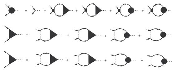
Figure 1: Dyson equations for full ordinary and anomalous vertices. The particle-hole interaction is shown by the shaded rectangle. Wavy lines represent the pairing interaction.

In these diagrams the shaded circle is the full ordinary vertex, and the shaded triangle represents the anomalous vertex. The particle-hole interaction is shown by the shaded rectangle. Wavy lines represent the pairing interaction. The first diagram on the right-hand side of the first line is the three-point vertex of a free particle.

In our analysis, we shall use the fact that the Fermi-liquid interactions do not interfere with the pairing phenomenon if approximate hole-particle symmetry is maintained in the system, i.e., the Fermi-liquid interactions remain unchanged upon pairing. Since we are interested in values of quasiparticle momenta near the Fermi surface, $\mathbf{p}\simeq p_{F}\mathbf{n}$, the Fermi-liquid effects are reduced to the standard particle-hole interactions:

$$\varrho\mathfrak{F}_{\alpha\gamma,\beta\delta}\left(\mathbf{nn}^{\prime}\right)=\mathfrak{f}\left(\mathbf{nn}^{\prime}\right)\delta_{\alpha\beta}\delta_{\gamma\delta}+\mathfrak{g}\left(\mathbf{nn}^{\prime}\right)\bm{\sigma}_{\alpha\beta}\bm{\sigma}_{\gamma\delta}~{}.$$

We are interested in excitations able to decay into neutrino pairs through neutral weak currents. Since the neutrino emission in the vector channel of weak interactions is strongly suppressed in nonrelativistic media L06 , L08 , L10a , we will focus on the interaction of the superfluid Fermi liquid with an external axial-vector field. In the nonrelativistic case, the bare axial-vector vertex is given by the spin matrices $\hat{\bm{\sigma}}$. (We neglect a small temporal component that arises as the relativistic correction.)

After the proper renormalization of the pairing interaction the equations for the axial-vector vertices can be reduced to the following analytic form (for brevity, we omit the dependence of functions on $\omega$ and $\mathbf{q}$ ):

$$\bm{\hat{\tau}}(\mathbf{n}) =\hat{\bm{\sigma}}+\hat{\bm{\sigma}}\int\frac{d\mathbf{n}^{\prime}}{8\pi}\mathfrak{g}\left(\mathbf{nn}^{\prime}\right)\left\{\mathcal{I}_{GF}\mathrm{Tr}\left[\hat{\bm{\sigma}}\hat{T}^{\left(1\right)}\hat{g}\left(\hat{\bm{\sigma}}\mathbf{\bar{b}}\right)\right]+\mathcal{I}_{FG}\mathrm{Tr}\left[\hat{\bm{\sigma}}\left(\hat{\bm{\sigma}}\mathbf{\bar{b}}\right)\hat{g}\hat{T}^{\left(2\right)}\right]\right.$$

$$\left.+\mathcal{I}_{GG}\mathrm{Tr}\left[\hat{\bm{\sigma}}\bm{\hat{\tau}}\right]+\mathcal{I}_{FF}\mathrm{Tr}\left[\hat{\bm{\sigma}}\left(\hat{\bm{\sigma}}\mathbf{\bar{b}}\right)\hat{g}\bm{\hat{\tau}}^{-}\hat{g}\left(\hat{\bm{\sigma}}\mathbf{\bar{b}}\right)\right]\right\}_{\mathbf{n}^{\prime}}~{},$$ (24)

$$\mathbf{\hat{T}}^{\left(1\right)}\left(\mathbf{n}\right) =\sum_{m_{j}}\hat{\bm{\sigma}}\mathbf{b}_{m_{j}}(\mathbf{n})\hat{g}V^{\left(r\right)}\int\frac{d\mathbf{n}^{\prime}}{8\pi}\left\{\mathcal{I}_{GG^{-}}\mathrm{Tr}\left[\hat{g}\left(\hat{\bm{\sigma}}\mathbf{b}_{m_{j}}^{\ast}\right)\mathbf{\hat{T}}^{\left(1\right)}\right]\right.$$

$$-\mathcal{I}_{FF}\mathrm{Tr}\left[\left(\hat{\bm{\sigma}}\mathbf{b}_{m_{j}}^{\ast}\right)\left(\hat{\bm{\sigma}}\mathbf{\bar{b}}\right)\hat{g}\mathbf{\hat{T}}^{\left(2\right)}\left(\hat{\bm{\sigma}}\mathbf{\bar{b}}\right)\right]$$

$$\left.-\mathcal{I}_{GF}\mathrm{Tr}\left[\left(\hat{\bm{\sigma}}\mathbf{b}_{m_{j}}^{\ast}\right)\bm{\hat{\tau}}\left(\hat{\bm{\sigma}}\mathbf{\bar{b}}\right)\right]+\mathcal{I}_{FG^{-}}\mathrm{Tr}\left[\left(\hat{\bm{\sigma}}\mathbf{b}_{m_{j}}^{\ast}\right)\left(\hat{\bm{\sigma}}\mathbf{\bar{b}}\right)\hat{g}\bm{\hat{\tau}}^{-}\hat{g}\right]\right\}_{\mathbf{n}^{\prime}}~{},$$ (25)

$$\mathbf{\hat{T}}^{\left(2\right)}\left(\mathbf{n}\right) =\sum_{m_{j}}\hat{g}\hat{\bm{\sigma}}\mathbf{b}_{m_{j}}^{\ast}(\mathbf{n})V^{\left(r\right)}\int\frac{d\mathbf{n}^{\prime}}{8\pi}\left\{\mathcal{I}_{G^{-}G}\mathrm{Tr}\left[\left(\hat{\bm{\sigma}}\mathbf{b}_{m_{j}}\right)\hat{g}\mathbf{\hat{T}}^{\left(2\right)}\right]\right.$$

$$-\mathcal{I}_{FF}\mathrm{Tr}\left[\left(\hat{\bm{\sigma}}\mathbf{b}_{m_{j}}\right)\left(\hat{\bm{\sigma}}\mathbf{\bar{b}}\right)\mathbf{\hat{T}}^{\left(1\right)}\hat{g}\left(\hat{\bm{\sigma}}\mathbf{\bar{b}}\right)\right]$$

$$\left.+\mathcal{I}_{G^{-}F}\mathrm{Tr}\left[\left(\hat{\bm{\sigma}}\mathbf{b}_{m_{j}}\right)\hat{g}\bm{\hat{\tau}}^{-}\hat{g}\left(\hat{\bm{\sigma}}\mathbf{\bar{b}}\right)\right]-\mathcal{I}_{FG}\mathrm{Tr}\left[\left(\hat{\bm{\sigma}}\mathbf{b}_{m_{j}}\right)\left(\hat{\bm{\sigma}}\mathbf{\bar{b}}\right)\bm{\hat{\tau}}\right]\right\}_{\mathbf{n}^{\prime}}~{}.$$ (26)

Inspection of the equations reveals that the solution should be of the form

$$\bm{\hat{\tau}}(\mathbf{n})=\phi\left(\mathbf{n}\right)\hat{\bm{\sigma}}\mathbf{~{},~{}}\hat{g}\bm{\hat{\tau}}^{-}\left(\mathbf{n}\right)\hat{g}=\phi\left(-\mathbf{n}\right)\hat{\bm{\sigma}}$$ (27)

$$\mathbf{\hat{T}}^{\left(1\right)}\left(\mathbf{n},\omega\right)=\sum_{m_{j}}\mathbf{B}_{m_{j}}^{\left(1\right)}\left(\omega\right)\left(\hat{\bm{\sigma}}\mathbf{b}_{m_{j}}\right)\hat{g}~{},$$ (28)

$$\mathbf{\hat{T}}^{\left(2\right)}\left(\mathbf{n},\omega\right)=\sum_{m_{j}}\mathbf{B}_{m_{j}}^{\left(2\right)}\left(\omega\right)\hat{g}\left(\hat{\bm{\sigma}}\mathbf{b}_{m_{j}}^{\ast}\right)~{}.$$ (29)

After this substitution and summation over spins, one can obtain a set of equations for

$$\phi_{\pm}\left(\mathbf{n}\right)=\frac{1}{2}\left(\phi\left(\mathbf{n}\right)\pm\phi(-\mathbf{n})\right)$$ (30)

and

$$\mathbf{B}_{m_{j}}^{\pm}=\frac{1}{2}\left(\mathbf{B}_{m_{j}}^{\left(1\right)}\pm\left(-\right)^{m_{j}}\mathbf{B}_{-m_{j}}^{\left(2\right)}\right)~{}.$$ (31)

The application of a little algebra using Eqs. (12)–(14) results in the following equations:

$$\phi_{+}\left(\mathbf{n}\right) =1+\int\frac{d\mathbf{n}^{\prime}}{4\pi}\mathfrak{g}\left(\mathbf{nn}^{\prime}\right)\left(\mathcal{I}_{GG}-\bar{b}^{2}\mathcal{I}_{FF}\right)_{\mathbf{n}^{\prime}}\phi_{+}\left(\mathbf{n}^{\prime}\right)$$

$$-\sum_{m_{j}}\mathbf{B}_{m_{j}}^{-}\frac{\omega}{\Delta}\int\frac{d\mathbf{n}^{\prime}}{4\pi}\mathfrak{g}\left(\mathbf{nn}^{\prime}\right)\mathcal{I}_{FF}\left(\mathbf{n}^{\prime}\right)i\left(\mathbf{b}_{m_{j}}\mathbf{\times\bar{b}}\right)_{\mathbf{n}^{\prime}}~{},$$ (32)

$$\phi_{-}\left(\mathbf{n}\right) =\int\frac{d\mathbf{n}^{\prime}}{4\pi}\mathfrak{g}\left(\mathbf{nn}^{\prime}\right)\left(\mathcal{I}_{GG}+\bar{b}^{2}\mathcal{I}_{FF}\right)_{\mathbf{n}^{\prime}}\phi_{-}\left(\mathbf{n}^{\prime}\right)$$

$$+\sum_{m_{j}}\mathbf{B}_{m_{j}}^{+}\int\frac{d\mathbf{n}^{\prime}}{4\pi}\mathfrak{g}\left(\mathbf{nn}^{\prime}\right)\frac{\mathbf{qv}}{\Delta}\mathcal{I}_{FF}\left(\mathbf{n}^{\prime}\right)i\left(\mathbf{b}_{m_{j}}\mathbf{\times\bar{b}}\right)_{\mathbf{n}^{\prime}}~{},$$ (33)

$$\sum_{m_{j}^{\prime}}\mathbf{B}_{m_{j}^{\prime}}^{+}\left[\int\frac{d\mathbf{n}}{4\pi}\left(\mathbf{b}_{m_{j}}^{\ast}\mathbf{b}_{m_{j}^{\prime}}-\delta_{m_{j},m_{j}^{\prime}}\frac{\Delta}{\Delta_{m_{j}}}\mathbf{b}_{m_{j}}^{\ast}\mathbf{\bar{b}}\right)A\right.$$

$$\left.+\int\frac{d\mathbf{n}}{4\pi}\left(\frac{\omega^{2}-\left(\mathbf{qv}\right)^{2}}{2\Delta^{2}}\mathbf{b}_{m_{j}}^{\ast}\mathbf{b}_{m_{j}^{\prime}}-2\left(\mathbf{b}_{m_{j}}^{\ast}\mathbf{\bar{b}}\right)\left(\mathbf{\bar{b}b}_{m_{j}^{\prime}}\right)\right)\mathcal{I}_{FF}\right]$$

$$=-2\int\frac{d\mathbf{n}}{4\pi}\left(\frac{\omega}{\Delta}\phi_{+}+\frac{\mathbf{qv}}{\Delta}\phi_{-}\right)i\left(\mathbf{b}_{m_{j}}^{\ast}\mathbf{\times\bar{b}}\right)\mathcal{I}_{FF}~{},$$ (34)

$$\sum_{m_{j}^{\prime}}\mathbf{B}_{m_{j}^{\prime}}^{-}\left[\int\frac{d\mathbf{n}}{4\pi}\left(\mathbf{b}_{m_{j}}^{\ast}\mathbf{b}_{m_{j}^{\prime}}-\delta_{m_{j}m_{j}^{\prime}}\frac{\Delta}{\Delta_{m_{j}}}\mathbf{b}_{m_{j}}^{\ast}\mathbf{\bar{b}}\right)A\right.$$

$$\left.+\int\frac{d\mathbf{n}}{4\pi}\left(\left(\frac{\omega^{2}-\left(\mathbf{qv}\right)^{2}}{2\Delta^{2}}-2\bar{b}^{2}\right)\mathbf{b}_{m_{j}}^{\ast}\mathbf{b}_{m_{j}^{\prime}}+2\left(\mathbf{b}_{m_{j}}^{\ast}\mathbf{\bar{b}}\right)\left(\mathbf{\bar{b}b}_{m_{j}^{\prime}}\right)\right)\mathcal{I}_{FF}\right]=0~{}.$$ (35)

In obtaining the last two equations, we used the gap equation (22) and the identity (15).

Further simplifications are possible due to the fact that $\mathbf{B}_{m_{j}}^{-}$ in Eq. (35) do not couple to external fields. Even if the eigenoscillations of $\mathbf{B}_{m_{j}}^{-}$ exist it is unclear how this mode could be excited. Therefore one may assume that Eq. (35) has only the trivial solution $\mathbf{B}_{m_{j}}^{-}=0$. This simplifies Eq. (32) which is now uncoupled.

The amplitudes of Fermi-liquid interactions can be expanded into Legendre polynomials and written in terms of an infinite set of Landau parameters. In the axial channel, this gives

$$\mathfrak{g}\left(\mathbf{nn}^{\prime}\right)=\sum_{l=0}^{\infty}\mathfrak{g}_{l}P_{l}\left(\mathbf{nn}^{\prime}\right)~{}.$$ (36)

We now expand the functions $\phi_{\pm}\left(\mathbf{n}\right)$ over spherical harmonics $Y_{lm}\left(\mathbf{n}\right)$. It is apparent that the function $\phi_{+}\left(\mathbf{n}\right)=\phi_{+}\left(-\mathbf{n}\right)$ contains only even harmonics,

$$\phi_{+}\left(\mathbf{n};\omega,\mathbf{q}\right)=\sqrt{4\pi}\sum_{l=\mathsf{even}}\sum_{m=-l}^{l}\phi_{l,m}^{+}\left(\omega,\mathbf{q}\right)Y_{l,m}\left(\mathbf{n}\right)~{},$$ (37)

while $\phi_{-}\left(\mathbf{n}\right)=-\phi_{-}\left(-\mathbf{n}\right)$ consists of odd harmonics,

$$\phi_{-}\left(\mathbf{n};\omega,\mathbf{q}\right)=\sqrt{4\pi}\sum_{l=\mathsf{odd}}\sum_{m=-l}^{l}\phi_{l,m}^{-}\left(\omega,\mathbf{q}\right)Y_{l,m}\left(\mathbf{n}\right)~{}.$$ (38)

Making use of the relation

$$\int d\mathbf{n}Y_{\lambda,\mu}^{\ast}\left(\mathbf{n}\right)\mathfrak{g}\left(\mathbf{nn}^{\prime}\right)=\sum_{l}\frac{4\pi}{2l+1}\mathfrak{g}_{l}\delta_{\lambda,l}Y_{l,\mu}^{\ast}\left(\mathbf{n}^{\prime}\right)~{},$$

which follows from the expansion (36), we arrive at the final set of of equations,

$$\phi_{l,m}^{+}=\delta_{l,0}\delta_{m,0}+\frac{\mathfrak{g}_{l}}{2l+1}\sum_{l^{\prime}=\mathsf{even}}\sum_{m^{\prime}}\phi_{l^{\prime},m^{\prime}}^{+}\int d\mathbf{n}Y_{l,m}^{\ast}\left(\mathcal{I}_{GG}-\bar{b}^{2}\mathcal{I}_{FF}\right)Y_{l^{\prime},m^{\prime}}~{},$$ (39)

$$\phi_{l,m}^{-} =\frac{\mathfrak{g}_{l}}{2l+1}\sum_{l^{\prime}=\mathsf{odd}}\sum_{m^{\prime}}\phi_{l^{\prime},m^{\prime}}^{-}\int d\mathbf{n}Y_{l,m}^{\ast}\left(\mathcal{I}_{GG}+\bar{b}^{2}\mathcal{I}_{FF}\right)Y_{l^{\prime},m^{\prime}}$$

$$+\frac{\sqrt{4\pi}\mathfrak{g}_{l}}{2l+1}i\frac{q\upsilon_{F}}{\Delta}\sum_{m_{j}}\mathbf{B}_{m_{j}}^{+}\int\frac{d\mathbf{n}}{4\pi}\left(\cos\theta_{\mathbf{qn}}\right)\left(\mathbf{b}_{m_{j}}\mathbf{\times\bar{b}}\right)\mathcal{I}_{FF}Y_{l,m}^{\ast}~{},$$ (40)

$$\sum_{m_{j}^{\prime}}\mathbf{B}_{m_{j}^{\prime}}^{+}\left[\int\frac{d\mathbf{n}}{4\pi}\left(\mathbf{b}_{m_{j}}^{\ast}\mathbf{b}_{m_{j}^{\prime}}-\delta_{m_{j},m_{j}^{\prime}}\frac{\Delta}{\Delta_{m_{j}}}\mathbf{b}_{m_{j}}^{\ast}\mathbf{\bar{b}}\right)A\right.$$

$$\left.+\int\frac{d\mathbf{n}}{4\pi}\left(\frac{\omega^{2}-q^{2}\upsilon_{F}^{2}\left(\cos\theta_{\mathbf{qn}}\right)^{2}}{2\Delta^{2}}\mathbf{b}_{m_{j}}^{\ast}\mathbf{b}_{m_{j}^{\prime}}-2\left(\mathbf{b}_{m_{j}}^{\ast}\mathbf{\bar{b}}\right)\left(\mathbf{\bar{b}b}_{m_{j}^{\prime}}\right)\right)\mathcal{I}_{FF}\right]$$

$$=-2i\sqrt{4\pi}\sum_{l=\mathsf{even}}\sum_{m}\phi_{l,m}^{+}\frac{\omega}{\Delta}\int\frac{d\mathbf{n}}{4\pi}\left(\mathbf{b}_{m_{j}}^{\ast}\mathbf{\times\bar{b}}\right)\mathcal{I}_{FF}Y_{l,m}$$

$$-2i\sqrt{4\pi}\sum_{l=\mathsf{odd}}\sum_{m}\phi_{l,m}^{-}\frac{q\upsilon_{F}}{\Delta}\int\frac{d\mathbf{n}}{4\pi}\left(\cos\theta_{\mathbf{qn}}\right)\left(\mathbf{b}_{m_{j}}^{\ast}\mathbf{\times\bar{b}}\right)\mathcal{I}_{FF}Y_{l,m}~{},$$ (41)

where $\theta_{\mathbf{qn}}$ is the angle between the transferred momentum and the direction of quasiparticle motion.

Since $l$ can take all values from zero to infinity, a general solution cannot be given in closed form. As in the case of a normal Fermi-liquid, a closed solution may be obtained if we set $\mathfrak{g}_{l}=0$ for $l>1$. We adopt this approximation and consider the solutions with $\mathbf{q=0}$.

With the aid of Eqs. (17)–(19), we find $\phi_{l,m}^{-}=0$ and

$$\phi_{0,0}^{+}=\frac{1}{1+2\mathfrak{g}_{0}\left\langle\bar{b}^{2}\mathcal{I}\left(\mathbf{n};\omega\right)\right\rangle}~{};~{}\phi_{l,m}^{+}=0~{},~{}l>0~{}.$$ (42)

Hereafter the angle brackets denote angle averages, $\left\langle...\right\rangle\equiv\left(4\pi\right)^{-1}\int d\mathbf{n}...$. Inserting these functions in Eq. (41) we obtain the set of equations for $\mathbf{B}_{m_{j}}^{+}$,

$$\sum_{m_{j}^{\prime}}\mathbf{B}_{m_{j}^{\prime}}^{+}\left[\left\langle\left(\mathbf{b}_{m_{j}}^{\ast}\mathbf{b}_{m_{j}^{\prime}}\right)A\right\rangle-\delta_{m_{j},m_{j}^{\prime}}\frac{\Delta}{\Delta_{m_{j}}}\left\langle\left(\mathbf{b}_{m_{j}}^{\ast}\mathbf{\bar{b}}\right)A\right\rangle\right.$$

$$\left.+\frac{\omega^{2}}{2\Delta^{2}}\left\langle\left(\mathbf{b}_{m_{j}}^{\ast}\mathbf{b}_{m_{j}^{\prime}}\right)\mathcal{I}\right\rangle-2\left\langle\left(\mathbf{b}_{m_{j}}^{\ast}\mathbf{\bar{b}}\right)\left(\mathbf{\bar{b}b}_{m_{j}^{\prime}}\right)\mathcal{I}\right\rangle\right]$$

$$=\frac{-2i}{1+2\mathfrak{g}_{0}\left\langle\bar{b}^{2}\mathcal{I}\right\rangle}\frac{\omega}{\Delta}\left\langle\left(\mathbf{b}_{m_{j}}^{\ast}\mathbf{\times\bar{b}}\right)\mathcal{I}\right\rangle~{}.$$ (43)

The unit vector $\mathbf{\bar{b}}$ used here was defined by Eq. (6).

The explicit evaluation of Eq. (43) for arbitrary values of $\omega$ and $T$ appears to require numerical computation. However, we can get a clear idea of the behavior of this function using the angle-averaged energy gap $\Delta^{2}\bar{b}^{2}\rightarrow\left\langle\Delta^{2}\bar{b}^{2}\right\rangle=$ $\Delta^{2}$ in the quasiparticle energy (10). (Replacing the angle-dependent gap in the quasiparticle energy by its average has been found to be a good approximation Baldo , L10a , L10c .) In this approximation, the functions $\mathcal{I}\left(\omega,T;\mathbf{n}\right)\rightarrow\mathcal{I}_{\mathsf{av}}\left(\omega,T\right)$ and $A\left(T\right)$, in Eqs. (42) and (43), can be moved beyond the angle integrals. With the aid of normalization condition (7), we find

$$\phi_{0,0}^{+}\left(\omega,T\right)=\frac{1}{1+2\mathfrak{g}_{0}\mathcal{I}_{\mathsf{av}}}~{}.$$ (44)

Using also the fact that

$$\left\langle\mathbf{b}_{m_{j}}^{\ast}\mathbf{b}_{m_{j}^{\prime}}\right\rangle=\delta_{m_{j}m_{j}^{\prime}}~{},~{}\frac{\Delta}{\Delta_{m_{j}}}\left\langle\mathbf{b}_{m_{j}}^{\ast}\mathbf{\bar{b}}\right\rangle=1$$ (45)

and substituting

$$\mathbf{B}_{m_{j}}^{+}\equiv\frac{1}{1+2\mathfrak{g}_{0}\mathcal{I}_{\mathsf{av}}}\mathbf{B}_{m_{j}}~{},$$

from Eq. (43), we obtain the set of linear equations for $\mathbf{B}_{m_{j}}$ with $m_{j}=0,\pm 1,\pm 2$,

$$\frac{\omega^{2}}{4\Delta^{2}}\mathbf{B}_{m_{j}}-\sum_{m_{j}^{\prime}}\mathbf{B}_{m_{j}^{\prime}}\left\langle\left(\mathbf{b}_{m_{j}}^{\ast}\mathbf{\bar{b}}\right)\left(\mathbf{\bar{b}b}_{m_{j}^{\prime}}\right)\right\rangle=-i\frac{\omega}{\Delta}\left\langle\mathbf{b}_{m_{j}}^{\ast}\mathbf{\times\bar{b}}\right\rangle~{}.$$ (46)

For further progress, we need to define a particular form of vector $\mathbf{\bar{b}}$ that characterizes the ground state of the condensate. The general form of a unitary ${}^{3}P_{2}$ state is to be written as

$$\mathbf{\bar{b}}=\frac{\Delta_{0}}{\Delta}\mathbf{b}_{0}+\frac{\Delta_{1}}{\Delta}\left(\mathbf{b}_{1}-\mathbf{b}_{-1}\right)+\frac{\Delta_{2}}{\Delta}\left(\mathbf{b}_{2}+\mathbf{b}_{-2}\right)$$ (47)

with

$$\Delta^{2}=\Delta_{0}^{2}+2\Delta_{1}^{2}+2\Delta_{2}^{2}~{}.$$ (48)

By utilizing notation adopted in Refs. Khodel , Clark , where $\lambda_{1}\equiv\sqrt{6}\Delta_{1}/\Delta_{0}$ and $\lambda_{2}\equiv\sqrt{6}\Delta_{2}/\Delta_{0}$, from Eq. (47) we obtain the general form of the properly normalized vector $\mathbf{\bar{b}}$:

$$\mathbf{\bar{b}}=\sqrt{\frac{1}{2}}\frac{\Delta_{0}}{\Delta}\left(\begin{array}[c]{ccc}-n_{1}+n_{1}\lambda_{2}-n_{3}\lambda_{1}~{},&-n_{2}-n_{2}\lambda_{2}~{},&2n_{3}-n_{1}\lambda_{1}\end{array}\right)~{}.$$ (49)

The solution to the set of linear equations (46) is found to be

$$\mathbf{B}_{0}=-\frac{1}{2}\bar{\omega}\frac{\Delta_{0}^{3}}{\Delta^{3}}\frac{\lambda_{1}}{\bar{\omega}^{2}-\bar{\omega}_{0}^{2}}\left(0,i,0\right)$$ (50)

$$\mathbf{B}_{\pm 1}=\frac{1}{4}\sqrt{\frac{2}{3}}\bar{\omega}\frac{\Delta_{0}^{3}}{\Delta^{3}}\left(-\frac{\left(3+\lambda_{2}\right)\left(\bar{\omega}^{2}-\bar{\omega}_{3}^{2}\right)}{\left(\bar{\omega}^{2}-\bar{\omega}_{1}^{2}\right)\left(\bar{\omega}^{2}-\bar{\omega}_{2}^{2}\right)},\frac{\pm i\left(3-\lambda_{2}\right)}{\bar{\omega}^{2}-\bar{\omega}_{0}^{2}},-\frac{\lambda_{1}\left(\bar{\omega}^{2}-\bar{\omega}_{4}^{2}\right)}{\left(\bar{\omega}^{2}-\bar{\omega}_{1}^{2}\right)\left(\bar{\omega}^{2}-\bar{\omega}_{2}^{2}\right)}\right)$$ (51)

$$\mathbf{B}_{\pm 2}=\mp\frac{1}{4}\sqrt{\frac{2}{3}}\bar{\omega}\frac{\Delta_{0}^{3}}{\Delta^{3}}\left(\frac{\lambda_{1}\left(\bar{\omega}^{2}-\bar{\omega}_{4}^{2}\right)}{\left(\bar{\omega}^{2}-\bar{\omega}_{1}^{2}\right)\left(\bar{\omega}^{2}-\bar{\omega}_{2}^{2}\right)},\frac{\pm i\lambda_{1}}{\bar{\omega}^{2}-\bar{\omega}_{0}^{2}},\frac{2\lambda_{2}\left(\bar{\omega}^{2}-\bar{\omega}_{5}^{2}\right)}{\left(\bar{\omega}^{2}-\bar{\omega}_{1}^{2}\right)\left(\bar{\omega}^{2}-\bar{\omega}_{2}^{2}\right)}\right)~{},$$ (52)

where $\bar{\omega}\equiv\omega/\left(2\Delta\right)$, and we use the following notation:

$$\bar{\omega}_{0}^{2}=\frac{1}{20}\frac{\Delta_{0}^{2}}{\Delta^{2}}\left(1+\lambda_{2}\right)^{2}~{},$$ (53)

$$\bar{\omega}_{1}^{2}=\frac{1}{40}\frac{\Delta_{0}^{2}}{\Delta^{2}}\left(5+2\lambda_{1}^{2}-2\lambda_{2}+\lambda_{2}^{2}+\sqrt{\left(1+\lambda_{2}\right)^{2}\left(4\lambda_{1}^{2}+\left(\lambda_{2}-3\right)^{2}\right)}\right)~{},$$ (54)

$$\bar{\omega}_{2}^{2}=\frac{1}{40}\frac{\Delta_{0}^{2}}{\Delta^{2}}\left(5+2\lambda_{1}^{2}-2\lambda_{2}+\lambda_{2}^{2}-\sqrt{\left(1+\lambda_{2}\right)^{2}\left(4\lambda_{1}^{2}+\left(\lambda_{2}-3\right)^{2}\right)}\right)~{},$$ (55)

$$\bar{\omega}_{3}^{2}=\frac{\Delta_{0}^{2}}{\Delta^{2}}\left(\frac{1}{5}+\frac{\lambda_{1}^{2}}{10}\frac{2+\lambda_{2}}{3+\lambda_{2}}\right)~{},$$

$$\bar{\omega}_{4}^{2}=\frac{1}{20}\frac{\Delta_{0}^{2}}{\Delta^{2}}\left(\lambda_{1}^{2}+2\lambda_{2}+2\lambda_{2}^{2}+4\right)~{},$$

$$\bar{\omega}_{5}^{2}=\frac{1}{20}\frac{\Delta_{0}^{2}}{\Delta^{2}}\left(\left(1-\lambda_{2}\right)^{2}+\frac{\lambda_{1}^{2}}{2\lambda_{2}}\left(1+3\lambda_{2}\right)\right)~{}.$$

By taking into account that $\mathbf{B}_{m_{j}}^{-}=\mathbf{0}$, we have $\mathbf{B}_{m_{j}}^{\left(1\right)}=\left(-\right)^{m_{j}}\mathbf{B}_{-m_{j}}^{\left(2\right)}$ and

$$\mathbf{\hat{T}}^{\left(1\right)}\left(\mathbf{n},\omega\right)=\frac{1}{1+2g_{0}\mathcal{I}_{\mathsf{av}}}\sum_{m_{j}}\mathbf{B}_{m_{j}}\left(\omega\right)\left(\hat{\bm{\sigma}}\mathbf{b}_{m_{j}}\right)\hat{g}~{},$$ (56)

$$\mathbf{\hat{T}}^{\left(2\right)}\left(\mathbf{n},\omega\right)=\frac{1}{1+2g_{0}\mathcal{I}_{\mathsf{av}}}\sum_{m_{j}}\mathbf{B}_{m_{j}}\left(\omega\right)\hat{g}\left(\hat{\bm{\sigma}}\mathbf{b}_{m_{j}}\right)~{}.$$ (57)

In the last equation, the property (3) is used.

The full ordinary axial-vector vertices can also be simplified because $\phi_{l,m}^{-}=0$ and, therefore, $\phi(-\mathbf{n})=\phi(\mathbf{n})$. From Eqs. (37), (42), and (44), we find $\phi\left(\mathbf{n};\omega,\mathbf{q}\right)=\phi_{0,0}^{+}\left(\omega,\mathbf{q}\right)$ and, thus,

$$\mathbf{\hat{\tau}}(\mathbf{n},\omega)=\frac{1}{1+2\mathfrak{g}_{0}\mathcal{I}_{\mathsf{av}}}\hat{\bm{\sigma}}~{},~{}\mathbf{\hat{\tau}}^{-}\left(\mathbf{n},\omega\right)=\frac{1}{1+2\mathfrak{g}_{0}\mathcal{I}_{\mathsf{av}}}\hat{\bm{\sigma}}^{T}\mathbf{~{}.}$$

According to modern theories Khodel -0203046 , there are several multicomponent states that compete in energy depending on the temperature. Accordingly the phase transitions occur between these states when the temperature goes down. The possible phase states of the ${}^{3}P_{2}-^{3}F_{2}$ condensate are cataloged in Ref. Clark . Immediately below the critical temperature, the superfluid condensate can appear either in one of the two two-component phases,

$$O_{\pm 3}:~{}\frac{\Delta_{0}}{\Delta}=\frac{1}{2}\ ,~{}\lambda_{1}=0~{},~{}\lambda_{2}=\pm 3$$ (58)

or in the one-component phase,

$$m_{j}=0:~{}\Delta_{0}=1,~{}\lambda_{1}=0,~{}\lambda_{2}=0~{}.$$ (59)

These lowest-energy states are nearly degenerate. The higher group is composed of the phases

$$O_{1}:~{}\frac{\Delta_{0}}{\Delta}=\frac{5}{\sqrt{14}\sqrt{17-3\sqrt{21}}},~{}\lambda_{1}=\frac{3}{5}\sqrt{2\left(17-3\sqrt{21}\right)},~{}\lambda_{2}=\frac{3}{5}\left(\sqrt{21}-4\right)$$ (60)

and

$$O_{2}:~{}\frac{\Delta_{0}}{\Delta}=\frac{5}{\sqrt{14}\sqrt{17+3\sqrt{21}}},~{}\lambda_{1}=\frac{3}{5}\sqrt{2\left(17+3\sqrt{21}\right)},~{}\lambda_{2}=-\frac{3}{5}\left(\sqrt{21}+4\right)~{}.$$ (61)

According to the above calculations the energy split between the two groups shrinks along with the temperature decrease and results in the phase transition at $T=0.7T_{c}$.

The effective vertices and the polarization tensors for each of the above phases can be obtained with the aid of Eqs. (50)–(52) and (67). We found that for all of the above-mentioned phases, the anomalous vertices can be written universally in the form

$$\mathbf{B}_{m_{j}}=\left(\frac{\Delta_{0}}{\Delta}\right)^{2}\frac{\bar{\omega}}{\bar{\omega}^{2}-1/20}i\left\langle\mathbf{b}_{m_{j}}^{\ast}\mathbf{\times\bar{b}}\right\rangle$$ (62)

where

$$\left\langle\mathbf{b}_{0}^{\ast}\mathbf{\times\bar{b}}\right\rangle =-\frac{1}{2\sqrt{6}}\frac{\Delta_{0}}{\Delta}\left(0,\sqrt{6}\lambda_{1},0\right)\,,$$

$$\left\langle\mathbf{b}_{\pm 1}^{\ast}\mathbf{\times\bar{b}}\right\rangle =-\frac{1}{2\sqrt{6}}\frac{\Delta_{0}}{\Delta}\left(-i\left(3+\lambda_{2}\right),\mp\left(3-\lambda_{2}\right),-i\lambda_{1}\right)~{},$$

$$\left\langle\mathbf{b}_{\pm 2}^{\ast}\mathbf{\times\bar{b}}\right\rangle =-\frac{1}{2\sqrt{6}}\frac{\Delta_{0}}{\Delta}\left(\mp i\lambda_{1},-\lambda_{1},\mp 2i\lambda_{2}\right)~{}.$$ (63)

Poles of the anomalous vertex indicate eigenmodes of the order parameter. The pole at $\bar{\omega}^{2}=1/20$ signals the existence of undamped collective spin oscillations of the energy

$$\omega_{s}\left(q=0\right)=\frac{\Delta}{\sqrt{5}}~{}.$$ (64)

Three important conclusions follow immediately from this simple formula: (a) The spin-density waves are of the identical excitation energy in all phases of the superfluid neutron liquid. (b) Fermi-liquid interactions do not influence the spin-wave energy in the condensate. (c) The spin waves are kinematically able to decay into neutrino pairs through neutral weak currents.

V Polarization functions.

Unfortunately, the Landau parameter $\mathfrak{g}_{0}$ for the particle-hole interactions in asymmetric nuclear matter is unknown. Therefore, in evaluating neutrino energy losses, we simply neglect the Fermi-liquid effects by taking $\mathfrak{g}_{0}\rightarrow 0$ and consider the axial polarization in the BCS approximation. The latter can be obtained in the form L10a

$$\Pi_{\mathrm{A}}^{ij}\left(\omega\right) =4\varrho\left\langle\frac{1}{2}\left(\mathcal{I}_{GG}-\bar{b}^{2}\mathcal{I}_{FF}\right)\delta_{ij}+\bar{b}^{2}\mathcal{I}_{FF}\frac{\bar{b}_{i}\bar{b}_{j}}{\bar{b}^{2}}\right\rangle$$

$$-\varrho\left\langle\frac{\omega}{2\Delta}\mathcal{I}_{FF}\mathrm{Tr}\left[\hat{\sigma}_{i}\hat{T}_{j}^{\left(1\right)}\hat{g}\left(\hat{\bm{\sigma}}\mathbf{\bar{b}}\right)-~{}\hat{\sigma}_{i}\left(\hat{\bm{\sigma}}\mathbf{\bar{b}}\right)\hat{g}\hat{T}_{j}^{\left(2\right)}\right]\right\rangle~{},$$ (65)

where $i,j=1,2,3$ and the anomalous axial-vector vertices $\mathbf{\hat{T}}^{\left(1,2\right)}$ are given by Eqs. (56) and (57). As in the above, we focus on the case $\mathbf{q=0}$ and omit for brevity the dependence on $\mathbf{n}$ and $\omega$. By using Eq. (19) and applying a little algebra, we obtain

$$\Pi_{\mathrm{A}}^{ij}\left(\omega\right) =-4\varrho\left\langle\left(\delta^{ij}\bar{b}^{2}-\bar{b}^{i}\bar{b}^{j}\right)\mathcal{I}\right\rangle$$

$$+\frac{4\varrho\omega^{2}}{\left(\omega+i0\right)^{2}-\Delta^{2}/5}\frac{\Delta_{0}^{2}}{\Delta^{2}}\sum_{m_{j}}\left\langle\left(\mathbf{b}_{m_{j}}\mathbf{\times\bar{b}}\right)^{i}\mathcal{I}\right\rangle\left\langle\mathbf{b}_{m_{j}}^{\ast}\mathbf{\times\bar{b}}\right\rangle^{j}~{}.$$

The pole location on the complex $\omega$ plane is chosen to obtain the retarded polarization tensor.

For further evaluation of the polarization function we will again use the angle-average approximation by replacing the angle-dependent gap in the quasiparticle energy (10) with its angle average, $\bar{b}^{2}\Delta^{2}\rightarrow\left\langle\bar{b}^{2}\Delta^{2}\right\rangle=\Delta^{2}$. Then the function

$$\mathcal{I}_{\mathsf{av}}\left(\omega\right)=\int_{0}^{\infty}\frac{d\varepsilon}{E}\frac{\Delta^{2}}{4E^{2}-\left(\omega+i0\right)^{2}}\tanh\frac{E}{2T}~{}$$ (66)

with $E^{2}=\varepsilon^{2}+4\Delta^{2}$, is isotropic and can be moved beyond the angle integral. In this approximation, we obtain

$$\Pi_{\mathrm{A}}^{ij}\left(\omega\right) =-4\varrho\left(\delta^{ij}-\left\langle\bar{b}^{i}\bar{b}^{j}\right\rangle\right)\mathcal{I}_{\mathsf{av}}\left(\omega\right)$$

$$+\frac{4\varrho\omega^{2}}{\left(\omega+i0\right)^{2}-\Delta^{2}/5}\mathcal{I}_{\mathsf{av}}\left(\omega\right)\frac{\Delta_{0}^{2}}{\Delta^{2}}\sum_{m_{j}}\left\langle\mathbf{b}_{m_{j}}\mathbf{\times\bar{b}}\right\rangle^{i}\left\langle\mathbf{b}_{m_{j}}^{\ast}\mathbf{\times\bar{b}}\right\rangle^{j}~{}.$$ (67)

Below we use the retarded polarization tensor for calculation of the neutrino energy losses from superfluid bulk matter of neutron stars. In this calculation one can neglect the temporal and mixed components of the tensor occurring as small relativistic corrections L09 .

VI Neutrino energy losses

We will examine the neutrino energy losses in the standard model of weak interactions. Then after integration over the phase volume of freely escaping neutrinos and antineutrinos the total energy which is emitted per unit volume and time can be obtained in the form (see details, e.g., in Ref. L01 )

$$\epsilon=-\frac{G_{F}^{2}C_{A}^{2}\mathcal{N}_{\nu}}{192\pi^{5}}\int_{0}^{\infty}d\omega\int d^{3}q\frac{\omega\Theta\left(\omega-q\right)}{\exp\left(\frac{\omega}{T}\right)-1}\operatorname{Im}\Pi_{\mathrm{A}}^{\mu\nu}\left(\omega,\mathbf{q}\right)\left(k_{\mu}k_{\nu}-k^{2}g_{\mu\nu}\right)~{},$$ (68)

where $G_{F}$ is the Fermi coupling constant, $C_{A}=1.26$ is the axial-vector weak coupling constant of neutrons, $\mathcal{N}_{\nu}=3$ is the number of neutrino flavors, $\Theta\left(x\right)$ is the Heaviside step function, and $k^{\mu}=\left(\omega,\mathbf{q}\right)$ is the total energy and momentum of the freely escaping neutrino pair $\left(\mu,\nu=0,1,2,3\right)$.

In Eq. (68), we have neglected the neutrino emission in the vector channel, which is strongly suppressed due to conservation of the vector current. Therefore the energy losses are connected to the imaginary part of the retarded polarization tensor in the axial channel, $\Pi_{\mathrm{A}}^{\mu\nu}\simeq\delta^{\mu i}\delta^{\nu j}\operatorname{Im}\Pi_{\mathrm{A}}^{ij}$. The latter is caused by the pair breaking and formation (PBF) processes and by the spin-wave decays (SWDs). These processes operate in different kinematical domains, so that the imaginary part of the polarization tensor consists of two clearly distinguishable contributions, $\operatorname{Im}\Pi_{\mathrm{A}}^{ij}=\operatorname{Im}\Pi_{\mathrm{PBF}}^{ij}+\operatorname{Im}\Pi_{\mathrm{SWD}}^{ij}$, which we will now consider.

VI.1 PBF channel

The imaginary part of $\mathcal{I}_{\mathsf{av}}$, which arises from the poles of the integrand in Eq. (66) at $\omega=\pm 2E$ is given by

$$\operatorname{Im}\mathcal{I}_{\mathsf{av}}\left(\omega>0\right)=\frac{\pi}{2}\frac{\Delta^{2}\Theta\left(\omega^{2}-4\Delta^{2}\right)}{\omega\sqrt{\omega^{2}-4\Delta^{2}}}\tanh\frac{\omega}{4T}~{}.$$

The PBF processes occur if $\omega>2\Delta$, while the energy (64) of the spin waves is considerably smaller. Therefore we may neglect the term $\allowbreak\Delta^{2}/5$ relative to $\omega^{2}$ in the denominator of Eq. (67). Then,

$$\operatorname{Im}\Pi_{ij}^{\mathrm{PBF}}\left(\omega\right) =-2\pi\varrho\left(\delta_{ij}-\left\langle\bar{b}_{i}\bar{b}_{j}\right\rangle-\frac{\Delta_{0}^{2}}{\Delta^{2}}\Lambda_{ij}\right)$$

$$\times\frac{\Delta^{2}\Theta\left(\omega^{2}-4\Delta^{2}\right)}{\omega\sqrt{\omega^{2}-4\Delta^{2}}}\tanh\frac{\omega}{4T}~{},$$ (69)

where

$$\Lambda_{ij}\equiv\sum_{m_{j}}\left\langle\mathbf{b}_{m_{j}}\mathbf{\times\bar{b}}\right\rangle_{i}\left\langle\mathbf{b}_{m_{j}}^{\ast}\mathbf{\times\bar{b}}\right\rangle_{j}$$

The tensors $\left\langle\bar{b}_{i}\bar{b}_{j}\right\rangle$ and $\Lambda_{ij}$ can be found with the aid of Eqs. (49) and (63). A straightforward calculation gives

$$\left\langle\bar{b}_{i}\bar{b}_{i}\right\rangle=\frac{1}{6}\frac{\Delta_{0}^{2}}{\Delta^{2}}\left(\begin{array}[c]{ccc}1-2\lambda_{2}+\lambda_{2}^{2}+\lambda_{1}^{2}&0&-\lambda_{1}-\lambda_{1}\lambda_{2}\\ 0&1+2\lambda_{2}+\lambda_{2}^{2}&0\\ -\lambda_{1}-\lambda_{1}\lambda_{2}&0&4+\lambda_{1}^{2}\end{array}\right)~{},$$ (70)

and

$$\Lambda_{ij}=\frac{1}{12}\frac{\Delta_{0}^{2}}{\Delta^{2}}\left(\begin{array}[c]{ccc}\lambda_{1}^{2}+\left(\lambda_{2}+3\right)^{2}&0&3\lambda_{1}\left(\lambda_{2}+1\right)\\ 0&4\lambda_{1}^{2}+\left(\lambda_{2}-3\right)^{2}&0\\ 3\lambda_{1}\left(\lambda_{2}+1\right)&0&\lambda_{1}^{2}+4\lambda_{2}^{2}\end{array}\right)~{}.$$ (71)

Inserting the imaginary part of the polarization tensor into Eq. (68), we calculate the contraction of $\operatorname{Im}\Pi_{\mathrm{PBF}}^{\mu\nu}$ with the symmetric tensor $k_{\mu}k_{\nu}-k^{2}g_{\mu\nu}$. This gives

$$\epsilon =\frac{1}{96\pi^{6}}G_{F}^{2}C_{A}^{2}\mathcal{N}_{\nu}p_{F}M^{\ast}\Delta^{2}\int_{0}^{\infty}\frac{d\omega}{\left(1+\exp\frac{\omega}{2T}\right)^{2}}\frac{\Theta\left(\omega^{2}-4\Delta^{2}\right)}{\sqrt{\omega^{2}-4\Delta^{2}}}$$

$$\times\int\limits_{q<\omega}d^{3}q\left(2\omega^{2}-q^{2}-q_{i}\left\langle\bar{b}_{i}\bar{b}_{i}\right\rangle q_{j}-\frac{3}{2}\frac{\Delta_{0}^{2}}{\Delta^{2}}\left(\omega^{2}-q^{2}\right)-\frac{\Delta_{0}^{2}}{\Delta^{2}}q_{i}\Lambda_{ij}q_{j}\right)~{}.$$ (72)

Integration over $d^{3}q$ can be done in cylindrical frame, where $q_{1}=q_{\perp}\cos\Phi$, $q_{2}=q_{\perp}\sin\Phi$, and $q_{3}=q_{z}$. This results in the neutrino energy losses in the form

$$\epsilon=\frac{1}{60\pi^{5}}\left(1-\frac{3}{4}\frac{\Delta_{0}^{2}}{\Delta^{2}}\right)G_{F}^{2}C_{A}^{2}\mathcal{N}_{\nu}p_{F}M^{\ast}\int_{2\Delta}^{\infty}\frac{\omega^{5}d\omega}{\left(1+\exp\frac{\omega}{2T}\right)^{2}}\frac{\Delta^{2}}{\sqrt{\omega^{2}-4\Delta^{2}}}~{}~{}.$$ (73)

In obtaining this expression, the following fact is used:

$$\frac{2}{3}\operatorname*{Tr}\Lambda_{ij}=\operatorname*{Tr}\left\langle\bar{b}_{i}\bar{b}_{i}\right\rangle=\frac{\Delta_{0}^{2}}{\Delta^{2}}\left(\frac{1}{3}\lambda_{1}^{2}+\frac{1}{3}\lambda_{2}^{2}+1\right)\equiv 1~{}.$$

With the aid of the change $\omega=2T\sqrt{x^{2}+\Delta^{2}/T^{2}}$, one can recast Eq. (73) into the form:

$$\epsilon_{\mathrm{PBF}}=\frac{2}{15\pi^{5}}\left(4-3\frac{\Delta_{0}^{2}}{\Delta^{2}}\right)G_{F}^{2}C_{A}^{2}\mathcal{N}_{\nu}p_{F}M^{\ast}T^{7}y^{2}\int_{0}^{\infty}\frac{z^{4}dx}{\left(1+\exp z\right)^{2}}$$ (74)

where $z=\sqrt{x^{2}+y^{2}}$ and $y=\Delta\left(T\right)/T$.

For a practical usage from Eq. (74), we find

$$\epsilon_{\mathrm{PBF}}=5.\,\allowbreak 85\times 10^{20}~{}\left(\frac{M^{\ast}}{M}\right)\left(\frac{p_{F}}{Mc}\right)T_{9}^{7}\mathcal{N}_{\nu}C_{\mathrm{A}}^{2}F_{\mathrm{PBF}}\left(y\right)~{}~{}~{}\frac{erg}{cm^{3}s}~{},$$ (75)

where $M$ and $M^{\ast}=p_{F}/\upsilon_{F}$ are the bare and effective nucleon masses, respectively; $T_{9}=T/10^{9}\mathrm{K}$, and

$$F_{\mathrm{PBF}}\left(y\right)=\left(4-3\frac{\Delta_{0}^{2}}{\Delta^{2}}\right)y^{2}\int_{0}^{\infty}dx\frac{z^{4}}{\left(1+\exp z\right)^{2}}\text{.}$$ (76)

The neutrino energy losses, as given by Eq. (74) with good accuracy reproduce the result obtained in Ref. L10a for the one-component phase $m_{j}=0$, where $\Delta_{0}/\Delta=1$. It is necessary to notice that Eq. (76) obtained in the angle-average approximation is much simpler for numerical evaluation than the ”exact” expression which contains additionally the angle integration L10a . To avoid possible misunderstanding we stress that the gap amplitude $\Delta\left(T\right)$ in Eq. (76) is $\sqrt{2}$ times larger than the gap amplitude $\Delta_{YKL}$ used in Ref. YKL , where the same anisotropic gap $\Delta_{\mathbf{n}}=\Delta\bar{b}\left(\mathbf{n}\right)$ is written in the form $\Delta_{\mathbf{n}}=\Delta_{YKL}\sqrt{1+3\cos^{2}\theta}\equiv\Delta_{YKL}\sqrt{2}\,\bar{b}\left(\mathbf{n}\right)$. In other words, $\left\langle\Delta_{\mathbf{n}}^{2}\right\rangle=\Delta^{2}=2\Delta_{YKL}^{2}$.

The small difference in the gap amplitudes, $\delta\Delta^{2}/\Delta^{2}\sim 2\%$, inherent for various phases of the condensate is crucial for the phase transitions 0203046 , but this small inequality can be disregarded in evaluation of the neutrino energy losses. Therefore the efficiency of PBF processes in various phases of the superfluid condensate is proportional to the factor

$$\kappa_{\mathrm{PBF}}\equiv 1-\frac{3}{4}\frac{\Delta_{0}^{2}}{\Delta^{2}}$$

For the one-component phase $m_{j}=0$ one has $\kappa_{\mathrm{PBF}}=1/4$; in the case of $O_{\pm 3}$ condensates, $\kappa_{\mathrm{PBF}}=13/16$. For the $O_{1}$ phase, we obtain $\kappa_{\mathrm{PBF}}=\left(173-9\sqrt{21}\right)/224\simeq 0.5882$, and for the $O_{2}$ phase, we have $\kappa_{\mathrm{PBF}}=\left(173+9\sqrt{21}\right)/224\simeq 0.95644$.

VI.2 SWD channel

In the frequency domain $0<\omega<\Delta\bar{b}$, the imaginary part of the weak polarization tensor (67) arises from the pole of the denominator at $\omega=\Delta/\sqrt{5}$ and can be written as

$$\operatorname{Im}\Pi_{ij}^{\mathrm{SWD}}\left(\omega>0\right)=-\frac{4}{5}\pi\sqrt{5}\Delta\varrho\delta\left(\omega-\Delta/\sqrt{5}\right)\mathcal{I}_{\mathsf{av}}\left(\omega\right)\frac{\Delta_{0}^{2}}{\Delta^{2}}\Lambda_{ij}~{}.$$ (77)

Inserting this expression into Eq. (68) and performing trivial calculations, we find

$$\epsilon_{\mathrm{SWD}}=\frac{G_{F}^{2}C_{A}^{2}\mathcal{N}_{\nu}}{160\pi^{5}}p_{F}M^{\ast}\frac{\Delta_{0}^{2}}{\Delta^{2}}\frac{\left(\Delta/\sqrt{5}\right)^{7}}{\exp\left(\frac{\Delta/\sqrt{5}}{T}\right)-1}\int_{0}^{\infty}\frac{d\varepsilon}{E}\frac{\Delta^{2}}{E^{2}-\Delta^{2}/20}\tanh\frac{E}{2T}~{}.$$ (78)

One can neglect $\Delta^{2}/20$ in comparison to $E^{2}>4\Delta^{2}$ in the denominator of the integrand. With this simplification, we obtain

$$\epsilon_{\mathrm{SWD}}=\frac{G_{F}^{2}\mathcal{N}_{\nu}}{160\pi^{5}}C_{A}^{2}p_{F}M^{\ast}T^{7}\frac{1}{\exp\left(y/\sqrt{5}\right)-1}\left(\frac{y}{\sqrt{5}}\right)^{7}\mathcal{I}_{0}\left(y\right)~{},$$ (79)

where $y\equiv\Delta\left(T\right)/T$, and

$$\mathcal{I}_{0}\left(y\right)=\int_{0}^{\infty}\frac{du}{\left(u^{2}+1\right)^{3/2}}\tanh\frac{y}{2}\sqrt{u^{2}+1}~{}.$$ (80)

This expression can be recast into the traditional form

$$\epsilon_{\mathrm{SWD}}=2.\,\allowbreak 74\times 10^{19}~{}\left(\frac{M^{\ast}}{M}\right)\left(\frac{p_{F}}{Mc}\right)T_{9}^{7}\mathcal{N}_{\nu}C_{\mathrm{A}}^{2}\frac{\Delta_{0}^{2}}{\Delta^{2}}\frac{\left(y/\sqrt{5}\right)^{7}\mathcal{I}_{0}\left(y\right)}{\exp\left(y/\sqrt{5}\right)-1}~{}~{}~{}\frac{erg}{cm^{3}s}~{}.$$ (81)

From this expression, it is seen that the efficieency of spin-wave decays is proportional to $\kappa_{\mathrm{SWD}}=\Delta_{0}^{2}/\Delta^{2}$. For the one-component condensate $m_{j}=0$, $\kappa_{\mathrm{SWD}}=1$; in the case of $O_{\pm 3}$ condensates, $\kappa_{\mathrm{SWD}}=1/4$. For the $O_{1}$ phase, we obtain $\kappa_{\mathrm{SWD}}=\left(17+3\sqrt{21}\right)/56\simeq\allowbreak 0.549\,07$, and for the $O_{2}$ phase, $\kappa_{\mathrm{SWD}}=\left(17-3\sqrt{21}\right)/56\simeq\allowbreak 5.81\times 10^{-2}$.

VII Phase transitions and efficiency of neutrino emission

For numerical evaluation of the neutrino losses, it is necessary to know the function $y=\Delta\left(T\right)/T$, which in general is to be found with the aid of gap equations. However, as mentioned above, the difference in the gap amplitudes for various phases can be neglected in evaluation of the neutrino energy losses. This substantially simplifies the problem because for the case $m_{j}=0$ the function is well investigated. We can adjust, for example, the simple fit to $\Delta_{YKL}\left(T\right)/T=\mathsf{v}_{B}\left(\tau\right)$, as suggested in Ref. YKL , where $\tau\equiv T/T_{c}$. Taking into account that, in Ref. YKL , the gap amplitude $\Delta_{YKL}\left(T\right)$ is defined by the relation $\Delta_{\mathbf{n}}^{2}=\Delta_{YKL}^{2}\left(1+3\cos^{2}\theta\right)$, while our definition is $\Delta_{\mathbf{n}}^{2}=\frac{1}{2}\Delta^{2}\left(1+3\cos^{2}\theta\right)$, we obtain $y\left(\tau\right)=\sqrt{2}\mathsf{v}_{B}\left(\tau\right)$.

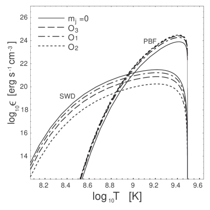
Figure 2: Temperature dependence of the neutrino emissivity due to recombination of Cooper pairs (PBF) and due to decay of spin waves (SWD) for $p_{F}=2.1~{}fm^{-1}$ and $T_{c}=3\times 10^{9}$ K. The effective mass is taken to be $M^{\ast}=0.7M$. The curves of different styles correspond to various phases of superfluid condensate, which are discussed in the text.

In Fig. 2 we compare the PBF and SWD neutrino emissivity for various phases of superfluid neutron matter. The temperature dependence of the emissivity is evaluated at $p_{F}=2.1fm^{-1}$. We set the effective nucleon masses $M^{\ast}=0.7M$; the critical temperature for neutron pairing is chosen to be $T_{c}=3\times 10^{9}K$.

One can see that the decay of spin waves into neutrino pairs is very effective at low temperatures, when other known mechanisms of neutrino energy losses in the bulk neutron matter are strongly suppressed by superfluidity. Maximal neutrino emission in the SWD channel occurs in the one-component phase. In contrast, efficiency of the PBF channel is maximal in the $O_{2}$ phase.

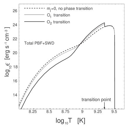
Figure 3: Total energy losses $\epsilon=\epsilon_{\mathrm{PBF}}+\epsilon_{\mathrm{SWD}}$ versus the temperature. The superfluid condensate undergoes the phase transition at $T=0.7T_{c}$. Parameters of the medium are the same as in Fig. 2.

In Fig. 3 we demonstrate the total neutrino emissivity $\epsilon=\epsilon_{\mathrm{PBF}}+\epsilon_{\mathrm{SWD}}$ versus the temperature by assuming that the phase transition occurs at $T=0.7T_{c}$. The phase transition (if it occurs) leads to a sharp increase in the neutrino energy losses followed by a decrease, along with a decrease in the temperature that takes place more rapidly than it would without the phase transition.

According to the minimal cooling paradigm Page04 , Page09 , along with lowering of the temperature, the star continues to lose its energy by radiating low-energy neutrinos via the PBF processes untill a photon-cooling epoch enters at $T\sim 0.1T_{c}$. At this latest stage of the cooling, all mechanisms of neutrino emission from the inner core are suppressed greatly by the neutron and proton superfluidity, and the $\gamma$ radiation from the star surface is considered as the main mechanism of the star cooling.

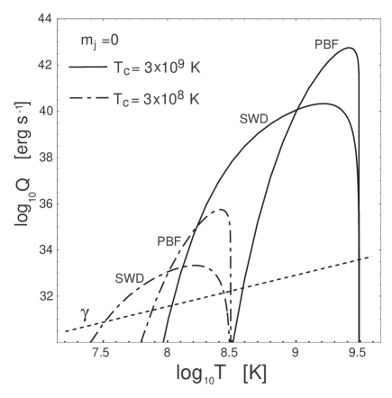
Figure 4: Temperature dependence of the neutrino luminosities from the model neutron star due to recombination of Cooper pairs (PBF) and due to decay of spin waves (SWD) for $p_{F}=2.1~{}fm^{-1}$. The effective mass is taken to be $M^{\ast}=0.7M$. Solid lines correspond to $T_{c}=3\times 10^{9}$ K; dot-dashed lines correspond to $T_{c}=3\times 10^{8}$ K. Volume of the triplet condensate is estimated as $7\times 10^{18}\ cm^{3}$. The dashed line is the energy losses per unit of time due to surface $\gamma$ radiation, as calculated in Ref. Page04 .

Given the strong dependence of the PBF and SWD neutrino emission on the temperature and the density, the overall effect of the SWD processes can only be assessed by complete calculations of the neutron star cooling which are beyond the scope of this paper. A rough estimate can be made by considering a simplified model of the superfluid core of the density $2\rho_{0}$ enclosed in the volume $7\times 10^{18}\ cm^{3}$. In Fig. 4 we demonstrate the total neutrino energy losses caused by PBF and SWD neutrino emission from the star volume in comparison with the surface photon radiation. The latter is taken as in Fig. 20 of Ref. Page04 . There is a relatively large range of predicted values for $T_{c}$; therefore, we show the PBF and SWD neutrino luminosities for $T_{c}=3\times 10^{9}$ K and for $T_{c}=3\times 10^{8}$ K. This simple estimate shows that the neutrino emission caused by spin-wave decay (SWD) can dominate the $\gamma$ radiation within some temperature range, which was previously considered as the photon-cooling era.

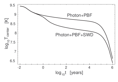
Figure 5: Transition of cooling trajectories between a model with a surface photon radiation and PBF neutrino emission and a model including a surface photon radiation and PBF+SWD neutrino processes. $T_{c}=3\times 10^{9}$ K. Details of the calculation are described in the text.

To get an idea of the lowering of the cooling trajectory due to SWD neutrino emission we consider a simple model of cooling of the above core of the density $2\rho_{0}$ and of the volume $7\times 10^{18}\ cm^{3}$ enclosed in a thin envelope typical for real neutron stars by assuming that the surface temperature is connected to the central temperature by the formula in Ref. Gudm . We assume also that the bulk matter consists mostly of ${}^{3}P_{2}$ superfluid neutrons with $m_{j}=0$ and contains a small admixture of normal (nonsuperfluid) protons and electrons (the proton fraction $x_{p}=0.05$), so that the total specific heat $C_{v}$ consists of the three corresponding contributions, as described in Ref. Yak99 . Under these conditions, the cooling equation

$$C_{v}\frac{dT}{dt}=-Q\ ,$$ (82)

can be solved numerically with $T=T_{c}$ at the initial moment. We have solved this equation for the case when $Q=Q_{\gamma}+Q_{PBF}$ and for the case when $Q=Q_{\gamma}+Q_{PBF}+Q_{SWD}$. The result is shown in Fig. 5.

VIII Summary and conclusion

Let us summarize our results. We have studied the linear response of the superfluid neutron liquid to an external axial-vector field. The calculation is made for the case of a multicomponent condensate involving several magnetic quantum numbers and allows us to consider various phases of superfluid neutron liquid. In order to estimate the neutrino energy losses, while taking into account possible phase transitions, we have considered the low-energy excitations of the multicomponent condensate.

Along with the well-known excitations in the form of broken Cooper pairs, we consider the collective waves of spin density, which are known to exist in the one-component condensate at very low energy L10b . Our theoretical analysis predicts the existence of such waves in all of the multicomponent phases we have considered. We found that the excitation energy of spin waves is identical for all of the phases and is independent of the Fermi-liquid interactions. In the angle-average approximation, the energy of spin-density oscillations is estimated as $\omega_{s}\left(q=0\right)\simeq\Delta/\sqrt{5}$.

Neutrino energy losses caused by the pair recombination and spin-wave decays are given by Eqs. (74) and (79), respectively. Because of a rather small excitation energy, the decay of spin waves leads to a substantial neutrino emission at the lowest temperatures $T\ll T_{c}$, when all other mechanisms of the neutrino energy losses are killed by a superfluidity. We have evaluated the neutrino energy losses for all of the multicomponent phases that might represent the ground state of the condensate according to modern theories.

Finally we have evaluated the temperature dependence of neutrino energy losses from the superfluid neutron liquid in the case when the phase transition occurs in the condensate at the temperature $T=0.7T_{c}$. Our estimate predicts a sharp increase of the neutrino energy losses followed by a decrease, along with a decrease of the temperature that takes place more rapidly than it would without the phase transition.

Since the neutron triplet-spin pairing occurs in the core which contains more than 90% of the neutron star volume, the neutrino processes discussed here could influence the evolution of neutron stars.

References

• (1) R. Tamagaki, Prog. Theor. Phys. 44 (1970) 905.
• (2) M. Hoffberg, A. E. Glassgold, R. W. Richardson, and M. Ruderman, Phys. Rev. Lett. 24 (1970) 775.
• (3) T. Takatsuka, Prog. Theor. Phys. 48 (1972) 1517.
• (4) M. Baldo, J. Cugnon, A. Lejeune and U. Lombardo, Nucl. Phys. A 536 (1992) 349.
• (5) Ø. ElgarΓΈy, L. Engvik, M. Hjorth-Jensen, E. Osnes, Nucl. Phys. A 607 (1996) 425.
• (6) D. Page, J. M. Lattimer, M. Prakash, A. W. Steiner, Astrophys. J. Supp. 155 (2004) 623.
• (7) D. Page, J. M. Lattimer, M. Prakash, A. W. Steiner, Astrophys. J. 707 (2009) 1131.
• (8) M.V. Zverev, J. W. Clark, and V. A. Khodel, Nucl. Phys. A 720 (2003) 20.
• (9) V. A. Khodel, J. W. Clark, and M.V. Zverev, Phys. Rev. Lett. 87 (2001) 031103.
• (10) V. A. Khodel, J. W. Clark, and M.V. Zverev, e:Print: arXiv:nucl-th/0203046.
• (11) D. G. Yakovlev, A. D. Kaminker, and K. P. Levenfish, Astron. Astrophys. 343 (1999) 650.
• (12) L. B. Leinson, Phys. Rev. C 81, 025501 (2010).
• (13) K. Maki and H. Ebisawa, J.Low Temp. Phys. 15 (1974) 213.
• (14) R. Combescot, Phys. Rev. A 10 (1974) 1700.
• (15) R. Combescot, Phys. Rev. Lett. 33 (1974) 946.
• (16) P. WΓΆlfe, Phys. Rev. Lett. 37 (1976) 1279.
• (17) P. WΓΆlfe, Physica B 90 (1977) 96.
• (18) L. B. Leinson, Phys. Lett. B 689 (2010) 60.
• (19) L. B. Leinson, e:Print: arXiv:hep-ph/1007.2803.
• (20) A. A. Abrikosov, L. P. Gorkov, I. E. Dzyaloshinkski, Methods of Quantum Field Theory in Statistical Physics, (Dover, New York, 1975).
• (21) A. B. Migdal, Theory of Finite Fermi Systems and Applications to Atomic Nuclei Β (Interscience, London, 1967).
• (22) A. J. Leggett, Phys. Rev. 140 (1965) 1869; Phys. Rev. 147 (1966) 119.
• (23) Y. Nambu, Phys. Rev. 117 (1960) 648.
• (24) A. I. Larkin and A. B. Migdal, Zh. Eksp. Teor. Fiz. 44 (1963) 1703 [Sov. Phys. JETP 17 (1963) 1146].
• (25) L. B. Leinson, Phys. Rev. C 79, 045502 (2009).
• (26) L. B. Leinson and A. PΓ©rez, Phys. Lett. B 638 (2006) 114.
• (27) L. B. Leinson, Phys. Rev. C 78, 015502 (2008).
• (28) L. B. Leinson, Nucl.Phys.A 687 (2001) 489.
• (29) E. H. Gudmundsson, C. J. Pethick, and R. I. Epstein, ApJ, 259 (1982) L19.
• (30) K. P. Levenfish and D. G. Yakovlev, Astron. Rep. 38 (1994) 247.