Casimir energy for a Regular Polygon with Dirichlet Boundaries

Abstract

We study the Casimir energy of a scalar field for a regular polygon with N sides. The scalar field obeys Dirichlet boundary conditions at the perimeter of the polygon. The polygon eigenvalues $\lambda_{N}$ are expressed in terms of the Dirichlet circle eigenvalues $\lambda_{C}$ as an expansion in $\frac{1}{N}$ of the form, $\lambda_{N}=\lambda_{C}{\,}(1+\frac{4{\,}\zeta(2)}{N^{2}}+\frac{4{\,}\zeta(3)}{N^{3}}+\frac{28{\,}\zeta(4)}{N^{4}}+\ldots{\,})$. A comparison follows between the Casimir energy on the polygon with $N=4$ found with our method and the Casimir energy of the scalar field on a square. We generalize the result to spaces of the form $R^{d}\times P_{N}$, with $P_{N}$ a N-polygon. By the same token, we find the electric field energy for a ”cylinder” of infinite length with polygonal section. With the method we use and in view of the results, it stands to reason to assume that the Casimir energy of $D$-balls has the same sign with the Casimir energy of regular shapes homeomorphic to the $D$-ball. We sum up and discuss our results at the end of the article.

Introduction

More than fifty years have passed since the article of H. Casimir [1] in which the force between conducting parallel plates was studied. The article was initially not so well known but the experiments where great advocates of its theoretical predictions and lead up to the establishment of the article making it a foundation for new research. The years that followed up to now where full of theoretical and experimental (for example see [2]) research towards the study of the so-called Casimir energy and Casimir force for various geometrical configurations [3]. Also the technological applications of the Casimir force are of great importance, for example in nanotubes, nano-devices in general and in microelectronic engineering [4]. Indeed it is obvious that the attractive or repulsive nature of the Casimir force can lead to the instability or even destruction of such a micro-device. In this manner, the study of various geometrical and material configurations will lead us to have control over the Casimir force, stabilizing the last by using appropriate geometrical structures.

The Casimir effect finds its explanation in the quantum structure of the vacuum. Indeed due to the fluctuations of the electromagnetic quantum field the parallel plates interact (in fact attracted towards each other). In addition it was of profound importance that the boundaries do alter the quantum field boundary conditions and as a result the plates interact. Indeed it was realized that the geometry of the boundaries have a strong effect in the Casimir energy and Casimir force, rendering the last repulsive or attractive. In Casimir’s work the force was attractive and some years later Boyer [5] studied the conducting sphere case, where it was found that the force is repulsive. These advisements where generalized to include other quantum fields such as fermions, bosons and other scalar fields making the Casimir effect study a widespread and necessary ingredient of many theoretical physics subjects such as string theory, cosmology [6, 7] e.t.c. For a concise treatment on these issues see for example [3, 6, 7, 8, 9] and references therein.

By now it is obvious that the boundary conditions affect drastically the Casimir force for all the aforementioned quantum fields. The most used boundary conditions are the Dirichlet and Neumann boundary conditions. However, these boundary conditions have no direct generalization in the case of fermion fields and in general for fields with spin$\neq 0$ [10]. In those cases, the bag boundary conditions are used which were introduced to provide a solution to confinement [11].

To our knowledge, up to date very few studies related to the Casimir energy for polygons where done. Some of them included the computation of the Casimir energy for hyperbolic polygons [12], also for tetrahedra [13] and for triangles [14]. The main difficulty was maybe the absence from the mathematical literature of the eigenvalue computation for regular polygons with Dirichlet boundaries. In this article we present one solution to such a problem, borrowed from the recent mathematical literature. This solution is found utilizing the calculus of moving surfaces [15, 16] which in our case is a perturbation of the circle with Dirichlet boundary conditions (from now on Dirichlet circle). The regular polygons are homeomorphic to the circle. This gives us the opportunity to model this by employing a kind of perturbation, as we mentioned. We shall see that the eigenvalues are expressed as a series in $1/N$, where $N$ stands for the number of sides of the regular polygon. When $N\rightarrow\infty$ we recover the Dirichlet circle’s eigenvalues as is expected, since the method is perturbative and does not rely to collapsing coordinates that parameterize the regular polygon when $N\rightarrow\infty$. As an application we shall compare our result for $N=4$ with the Casimir energy of a scalar filed in a Dirichlet square. A numerical and an analytic study of both will help us to make the comparison. A generalization of the Casimir energy for spaces of the form $R^{d}\times P_{N}$ follows ($P_{N}$ is the $N$-polygon).

The interest in studying the Casimir energy in such polygonal configurations stems from various applications, both theoretical and experimental and also from conceptual interest. The last is a good motivation because the curvature singularities that corners introduce are usually hard to handle and so being able to find solutions to Dirichlet problems in such configurations is quite a challenge. The theoretical applications are focused mainly in the fact that such spaces arise in the $1+2$ dimensional theory of gravity [13]. Also these spaces can be considered as triangulation approximations to smooth manifolds (in a way the last will be used in our article). Both experimentally and theoretically, polygonal configurations arise in superconducting regular polygons. We shall briefly discuss these issues later on in this article.

Laplace Eigenvalues on Regular Polygons and Casimir Energy

Consider the Laplace equation for a scalar field, solved for a circle, with the field obeying Dirichlet boundary conditions on the circle, namely:

$$-\Delta\Phi(x,y)=\lambda\Phi(x,y),$$ (1)

with $\Delta$, $\lambda$ and $\Phi(x,y)$, the Laplacian, the eigenvalues of the Laplacian and the scalar field respectively. It is much more convenient to express the equation and solutions in polar coordinates,

$$-\Delta\Phi(r,\phi)=\lambda\Phi(r,\phi).$$ (2)

Let $\lambda_{N}$ and $\lambda_{C}$ denote the eigenvalues of the problem corresponding to the Dirichlet regular polygon and to the Dirichlet circle respectively. The eigenvalues of the polygon $\lambda_{N}$ were studied in [15, 16] by employing the calculus of moving surfaces. According to this method the polygon is treated as a non-smooth perturbation of the circle. The problem was first studied by Hadamard in [17] and the solution is given as an integral over the mesh, that is, the area between the circle and the inscribed regular polygon:

$$\frac{\lambda_{N}}{\lambda_{C}}=\int\int_{C-P_{N}}|\mathrm{grad}{\,}u_{C}|\mathrm{d}x\mathrm{d}y.$$ (3)

Hadamard proved that the first correction to (3) is of order $\sim 1/N^{2}$. The authors of [15, 16] improved the solution of Hadamard, giving three more terms in the perturbation series, as we shall shortly see.

Without getting into much detail, let us shortly describe here the philosophy of the method. It is based on the calculus of moving surfaces. The key point is to find the shape derivative, the derivative of $\lambda$ as the boundary shape changes. The calculus of moving surfaces is based on the rate at which the boundary moves normal to itself. The last is fully described by the fundamental theorem for a moving surface $S$ bounding a region $\Omega$,

$$\frac{\mathrm{d}}{\mathrm{d}\tau}\int_{\Omega}F\mathrm{d}\Omega=\int_{\Omega}\frac{\partial F}{\partial\tau}{\,}\mathrm{d}\Omega+\int_{S}C{\,}F{\,}\mathrm{d}S.$$ (4)

In the above equation $C$ stands for the velocity of the boundary and $F$ is an invariant. Additionally to theorem (4) there exists the theorem,

$$\frac{\mathrm{d}}{\mathrm{d}\tau}\int_{\Omega}F\mathrm{d}S=\int_{S}\frac{\mathrm{\delta}F}{\mathrm{\delta}\tau}{\,}\mathrm{d}S-\int_{S}C{\,}B_{\alpha}^{\alpha}{\,}\mathrm{d}S.$$ (5)

Mention that the derivative $\frac{\mathrm{\delta}F}{\mathrm{\delta}\tau}$, is defined to act as follows,

$$\frac{\mathrm{\delta}F}{\mathrm{\delta}\tau}=\frac{\partial F}{\partial\tau}+C{\,}\frac{\partial F}{\partial n},$$ (6)

while $B_{\alpha}^{\alpha}$ is the trace of the curvature tensor $B^{\alpha}_{\beta}$. In brief, invariance on surfaces is achieved by introducing the covariant derivative $\nabla_{a}$, while invariance on moving surfaces can be achieved by using the $\delta/\delta\tau$ derivative, which was firstly introduced by Hadamard [17]. The $\delta/\delta\tau$ derivative acts on the invariant field $F$ of the moving surface. An invariant field of the surface can be for example, the mean curvature, the eigenfunction $\psi$ of the Laplace eigenvalue equation for the area $\Omega$, or the velocity of the surface boundary $C$. For more details consult references [15, 16] and references therein. We shall take the result of their method for computing the eigenvalues.

So making use of the method of moving surfaces and treating the polygon as a perturbation of the circle, the eigenvalues of the polygon $\lambda_{N}$ are related to the eigenvalues of the Dirichlet circle problem $\lambda_{C}$ according to the following series expansion in powers of $1/N$:

$$\lambda_{N}=\lambda_{C}{\,}(1+\frac{4{\,}\zeta(2)}{N^{2}}+\frac{4{\,}\zeta(3)}{N^{3}}+\frac{28{\,}\zeta(4)}{N^{4}}+\ldots{\,}),$$ (7)

where $\zeta$ is the Riemann zeta function [15, 16]. Call to mind that the eigenvalues $\lambda_{C}$ are the roots $\gamma_{mn}$ of the Bessel functions of the first kind $J_{m}(\gamma_{mn}{\,}r)$, and that $u_{C}\sim J_{m}(\gamma_{mn}{\,}r)e^{im\phi}$. The method works for the radial eigenfunctions, so the $\phi$ dependence is dropped, but this does not affect our analysis.

Before closing this section we must mention a drawback that such calculations have. It is the fact that there are singularities at the corners of the polygon. It is obvious that sharp corners introduce qualitatively new features that cannot be easily captured by perturbative techniques. However an infinitesimal smoothing of the corners does not alter the eigenfunctions concentrated away from the boundaries [15]. Likewise, the moving surfaces approach yields expressions that remain valid even for large eigenvalues (see [15] and references therein).

Casimir Energy

The Casimir energy for the regular polygon is the sum of the energy eigenvalues for that space with Dirichlet boundary conditions, that is,

$$E_{N}=\frac{1}{2}\sum_{n}\sqrt{\lambda_{N}^{(n)}},$$ (8)

where the sum over $n$ denotes all the modes that will be summed in the end. Substituting relation (7) in (8), we obtain:

$$E_{N}\simeq\frac{1}{2}\sum_{n}\sqrt{\lambda_{C}^{(n)}{\,}\Big{(}1+\frac{4{\,}\zeta(2)}{N^{2}}+\frac{4{\,}\zeta(3)}{N^{3}}+\frac{28{\,}\zeta(4)}{N^{4}}}\Big{)},$$ (9)

Recall that the Dirichlet circle Casimir energy is equal to:

$$E_{C}=\frac{1}{2}\sum_{n}\sqrt{\lambda_{C}^{(n)}},$$ (10)

hence the polygon Casimir energy reads,

$$E_{N}\simeq\sqrt{\Big{(}1+\frac{4{\,}\zeta(2)}{N^{2}}+\frac{4{\,}\zeta(3)}{N^{3}}+\frac{28{\,}\zeta(4)}{N^{4}}}\Big{)}E_{C}$$ (11)

In the large $N$ limit ($N\rightarrow\infty$), the regular polygon Casimir energy reads,

$$E_{N}\simeq E_{C}+\frac{7\pi^{4}}{45}\frac{1}{N}E_{C}+\frac{1350\pi^{2}-49\pi^{8}}{4050}\frac{1}{N^{2}}E_{C}+\ldots$$ (12)

By looking the above dependence it is obvious that the Dirichlet circle Casimir energy is recovered in the large $N$ limit of the regular polygon’s Casimir energy. To see how valid is the approximation we made in relation (11), let us compare the perturbative result of (11) for $N=4$ with the Casimir energy of a square area with Dirichlet boundary conditions on each side of the square. Take for simplicity that the radius of the circle is 1, thus the side of the square is $1$.

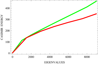
Figure 1: The Casimir energy of the polygon (green) and of the square (red) for $10^{4}$ eigenvalues

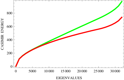
Figure 2: The Casimir energy of the polygon (green) and of the square (red) for $32400$ eigenvalues

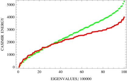
Figure 3: The Casimir energy of the polygon (green) and of the square (red) for $10^{6}$ eigenvalues

The eigenvalues of the Laplacian for the Dirichlet square are equal to:

$$\lambda_{s}=\frac{\pi}{a}\sqrt{m^{2}+n^{2}},$$ (13)

with $a=1$. The eigenvalues $\lambda_{C}$ of the Dirichlet unit circle are the roots of the Bessel function of first kind, $J_{n}(x_{nm})$, that is $\lambda_{C}=x_{nm}$. In such away, the polygon eigenvalues for $N=4$ considering the polygon as a circle perturbation are:

$$\lambda_{nm}\sim\sqrt{\Big{(}1+\frac{4{\,}\zeta(2)}{N^{2}}+\frac{4{\,}\zeta(3)}{N^{3}}+\frac{28{\,}\zeta(4)}{N^{4}}}\Big{)}x_{nm},$$ (14)

with $N=4$. Let us check how the eigenvalues (and accordingly the Casimir energy) behaves as a function of $n$ and $m$. In figures (1), (2) and (3) we plot the comparison of the first $10^{4}$, $32400$ and $10^{6}$ eigenvalues of the Dirichlet unit circle and the corresponding square ones. We can see how close the two plots are, proving that the approximation is quite valid. On that account, the perturbation of the circle eigenvalues gives results that fail to be truth for a percentage about $16.2\%$, as it is found numerically. Let us check the asymptotic form of eigenvalues. Remember that the asymptotic behavior of the Bessel’s function $J_{n}(x)$ roots is given by:

$$x_{mn}=n\pi+(m-\frac{1}{2})\frac{\pi}{2}.$$ (15)

and thereupon the polygon eigenvalues are:

$$\lambda_{nm}\sim\sqrt{\Big{(}1+\frac{4{\,}\zeta(2)}{N^{2}}+\frac{4{\,}\zeta(3)}{N^{3}}+\frac{28{\,}\zeta(4)}{N^{4}}}\Big{)}\Big{(}n\pi+(m-\frac{1}{2})\frac{\pi}{2}\Big{)}$$ (16)

We compare the above with these of relation (13) for various values of $n$ and $m$. For $n\gg m$, the square eigenvalues are equal to $\lambda_{s}\sim\pi n$, while the polygon’s are $\lambda_{nm}\sim n\pi\sqrt{\Big{(}1+\frac{4{\,}\zeta(2)}{N^{2}}+\frac{4{\,}\zeta(3)}{N^{3}}+\frac{28{\,}\zeta(4)}{N^{4}}}\Big{)}$ which for $N=4$ is approximately,

$$\lambda_{nm}\sim 1.26678{\,}n\pi.$$ (17)

Along these lines, we can see that the eigenvalues are approximately equal with a difference of $20\%$. For $m\sim n$, in which case $\lambda_{nm}$ becomes $\lambda_{nm}\sim 1.90017{\,}n\pi$ and also $\lambda_{s}\sim 2\pi n$. So the difference of the two above is approximately $5\%$. Now the only problem arises when $m\gg n$, in which case we have, $\lambda_{s}\sim\pi m$ and $\lambda_{nm}\sim 1.26678{\,}n\frac{\pi}{2}$. So the difference in these eigenvalues approaches $57\%$. However as we saw previously, the actual numerical difference is much smaller. In fact the numerical calculation performed for a very large range of eigenvalues gave a difference which approaches $16.2\%$. This result is adequate, in view of the fact that we are working with a perturbative method.

We give now a much more elaborate calculation of the Casimir energy for both the square and the polygon, using the zeta function regularization [6, 7, 8, 9]. In the case of the Bessel zeros sums, although the sum is explicit, the analytic continuation is not easy to do. The square Casimir energy can be done easily employing zeta regularization [6, 7, 8, 9].

Casimir energy of the Dirichlet circle $B_{2}$

Consider a scalar field obeying Dirichlet boundary conditions on a circle. We shall find the Casimir energy of the scalar field. With the same notation as above, the Casimir energy is equal to,

$$E_{C}=\frac{1}{2}\sum_{m,n}x_{m,n}.$$ (18)

The corresponding zeta function is,

$$\zeta(s)=\sum_{m,n}\lambda_{m,n}^{s}(a)-\sum_{m,n}\bar{\lambda}_{m,n}^{s}(\infty).$$ (19)

In the above, $\lambda_{m,n}(a)$ and $\bar{\lambda}_{m,n}(\infty)$ are the scalar field’s eigenvalues with Dirichlet boundaries and when the boundary is sent to infinity respectively. The Casimir energy can be written as,

$$E_{C}=\frac{1}{2}\zeta(s=-1).$$ (20)

Following the techniques developed in [18, 19], we find that,

$$\zeta(-1)=\frac{1}{\pi}\lim_{s\rightarrow 0}\sum_{i=0}^{3}Z_{i}(s)$$ (21)

with $Z_{0}$ to stand for,

$$Z_{0}(s)=-(1-s)\int_{0}^{\infty}\mathrm{d}y{\,}y^{-s}\Big{[}\ln(2y\mathrm{I}_{0}(y)\mathrm{K}_{0}(y))-\frac{t^{2}}{8}(1-6t^{2}+5t^{4})\Big{]},$$ (22)

$Z_{1}$ being equal to,

$$Z_{1}(s)=\frac{1-s}{2}\zeta(s-1)\Gamma(-\frac{1-s}{2})\sum_{m=1}^{\infty}\frac{\Gamma(m-\frac{1-s}{2})}{m\Gamma(m)},$$ (23)

$Z_{2}$ equal to,

$$Z_{2}(s)=\frac{1}{2}\big{(}\zeta(s+1)\frac{1}{2}\big{)}\Gamma(\frac{1+s}{2})(-1+3(1+s)-\frac{5}{8}(3+s)(1+s))$$ (24)

and finally $Z_{3}$,

$$Z_{3}(s)= \frac{1}{32}\zeta(s+3)\Gamma(\frac{3-s}{2})(-13\Gamma(\frac{3+s}{2})+142\Gamma(\frac{5+s}{2})-177\Gamma(\frac{7+s}{2})$$ (25)

$$+\frac{113}{2}\Gamma(\frac{9+s}{2})-\frac{113}{24}\Gamma(\frac{11+s}{2})).$$

In the above equation, $\mathrm{I}_{0}$ and $\mathrm{K}_{0}$ are the modified Bessel functions of first and second kind, and $t=1/\sqrt{1+y^{2}}$. Relations (22), (23), (24) and (25) for $s=0$ after numerical calculation and integration become (note that as $s\rightarrow 0$, $\zeta(1+s)\sim\frac{1}{s}+\gamma+\ldots$),

$$Z_{0}(0) =\pi(0.02815-\frac{1}{128}),{\,}{\,}{\,}Z_{1}(0)=-\frac{\pi}{12},{\,}{\,}{\,}$$ (26)

$$Z_{2}(0)=\frac{\pi}{64}(\frac{1}{s}+\gamma)+\frac{\pi}{128},{\,}{\,}{\,}Z_{3}(0)=-0.13679\frac{\pi}{64}\zeta(3).$$

Adding the above contributions we obtain,

$$\zeta(-1)=\frac{1}{a}\big{(}0.047189-\frac{1}{64{\,}s}\big{)},$$ (27)

and finally the Casimir energy is equal to,

$$E_{C}=\frac{1}{a}\big{(}0.023595-\frac{1}{128{\,}s}\big{)}.$$ (28)

The drawback of relation (27) in company with (28) is the existence of a pole. This fact makes someone to doubt about the validity of the above expressions. However it is the only way to obtain a clue of what the regularized Casimir energy looks like. But in the end the result is not to be trusted [18]. Like so, the numerical value of the Casimir energy $E_{C}$ for the unit circle is, $E_{C}=0.023595-\frac{1}{128{\,}s}$. Call to mind that the polygon Casimir energy is equal to,

$$E_{N}\simeq\sqrt{\Big{(}1+\frac{4{\,}\zeta(2)}{N^{2}}+\frac{4{\,}\zeta(3)}{N^{3}}+\frac{28{\,}\zeta(4)}{N^{4}}}\Big{)}E_{C},$$ (29)

hence we obtain that, $E_{N}\simeq 0.029769-\frac{1.266783}{128{\,}s}$.

Casimir energy of the Dirichlet square

In the case of the Casimir energy of a scalar field in a Dirichlet square, things are more easy and accurate compared to the Dirichlet circle case. Indeed the zeta function for the Dirichlet square is [6]:

$$\zeta(s)=\sum_{m,n}\Big{(}\frac{\pi^{2}m^{2}}{a^{2}}+\frac{\pi^{2}n^{2}}{a^{2}}\Big{)}^{-s}.$$ (30)

By virtue of the following asymptotic expansion,

$$\zeta_{EH}(s;p) =\frac{1}{2}\sum_{n=-\infty}^{\infty^{\prime}}\big{(}n^{2}+p\big{)}^{-s}$$ (31)

$$=-\frac{p^{-s}}{2}+\frac{\sqrt{\pi}{\,}{\,}\Gamma(s-\frac{1}{2})}{2\Gamma(s)}{\,}p^{-s+\frac{1}{2}}+\frac{2\pi^{s}{\,}p^{-s+\frac{1}{2}}}{\Gamma(s)}\sum_{n=1}^{\infty}n^{s-\frac{1}{2}}K_{s-\frac{1}{2}}\big{(}2\pi n\sqrt{p}\big{)},$$

relation (30) can be written as:

$$\zeta(s) =-\frac{1}{2}\Big{(}\frac{a}{\pi}\Big{)}^{2s}\zeta(2s)+\frac{a}{2\sqrt{\pi}}\Big{(}\frac{a}{\pi}\Big{)}^{2s-1}\frac{\Gamma(s-1/2)}{\Gamma(s)}\zeta(2s-1)$$ (32)

$$+\frac{2}{\Gamma(s)}\Big{(}\frac{a^{2}}{\pi}\Big{)}^{s}\sum_{m,n}\Big{(}\frac{m}{n}\Big{)}^{s-1/2}\mathrm{K}_{s-1/2}(2\pi mn),$$

with $\mathrm{K}_{\nu}$ the modified Bessel function. Thereupon, the numerical value of the Casimir energy $E_{S}$ for $a=1$ is $E_{S}=0.0415358$. Let us gather the results at this point. We take the finite part of the Dirichlet circle Casimir energy and we have that the difference in the Casimir energies of the polygon and of the square is approximately $28\%$, which is quite bigger than the one we found numerically earlier in this article (see below relation (17)). Of course we must note that the pole in the Dirichlet circle Casimir energy does not allow us to be sure of the $\frac{E_{S}-E_{N}}{E_{S}}$ difference. Consequently we must realize that the approximation we made in the beginning of this article,

$$\lambda_{N}=\lambda_{C}{\,}(1+\frac{4{\,}\zeta(2)}{N^{2}}+\frac{4{\,}\zeta(3)}{N^{3}}+\frac{28{\,}\zeta(4)}{N^{4}}+\ldots{\,}),$$ (33)

clearly holds with an $16.2\%$ accuracy for a wide range of modes, but a deeper investigation is needed to get a clear and accurate result on this.

The Casimir energy on $R^{{\,}D}\times P_{N}$ and on a Cylinder

Let us generalize the results of the previous section by considering a scalar field in a spacetime with topology $R^{{\,}D}\times P_{N}$, where $P_{N}$ denotes the regular polygon. The scalar field is assumed to obey Dirichlet boundary conditions on the regular polygon perimeter. We shall make use of the zeta function regularization method in order to obtain regularized results for the Casimir energy. We can write the Casimir energy for the total spacetime in the following form:

$$\mathcal{E}_{N}=\frac{1}{4\pi^{2}}\int\mathrm{d}^{D-1}p\sum_{m,n}\Big{[}\sum_{k=1}^{D-1}p_{k}^{2}+\lambda_{mn}\Big{]}^{-s}.$$ (34)

Remember that $\lambda_{mn}$ stand for the regular polygon eigenvalues. In addition we shall take $s=-1/2$ in the end in order to recover the Casimir energy. Upon integrating over the continuous dimensions utilizing the following,

$$\int\mathrm{d}k^{D-1}\frac{1}{(k^{2}+A)^{s}}=\pi^{\frac{D-1}{2}}\frac{\Gamma(s-\frac{D-1}{2})}{\Gamma(s)}\frac{1}{A^{s-\frac{D-1}{2}}}$$ (35)

relation (34) is reformed into,

$$\mathcal{E}_{N}=\frac{1}{4}\pi^{\frac{D-5}{2}}\frac{\Gamma(s-\frac{D-1}{2})}{\Gamma(s)}\sum_{m,n}\big{(}\lambda_{mn}\big{)}^{\frac{D-1}{2}-s}.$$ (36)

Bring to mind that,

$$\lambda_{mn}=x_{mn}{\,}(1+\frac{4{\,}\zeta(2)}{N^{2}}+\frac{4{\,}\zeta(3)}{N^{3}}+\frac{28{\,}\zeta(4)}{N^{4}}+\ldots{\,}),$$ (37)

where $x_{mn}$ stand for the Dirichlet circle eigenvalues. In virtue of the above two relations we obtain that,

$$\mathcal{E}_{N}\simeq\frac{1}{4}\pi^{\frac{D-5}{2}}\frac{\Gamma(s-\frac{D-1}{2})}{\Gamma(s)}\Big{(}1+\frac{4{\,}\zeta(2)}{N^{2}}+\frac{4{\,}\zeta(3)}{N^{3}}+\frac{28{\,}\zeta(4)}{N^{4}}\Big{)}^{\frac{D-1}{2}-s}\sum_{m,n}\big{(}x_{mn}\big{)}^{\frac{D-1}{2}-s}.$$ (38)

The expression,

$$\frac{1}{4}\pi^{\frac{D-5}{2}}\frac{\Gamma(s-\frac{D-1}{2})}{\Gamma(s)}\sum_{m,n}\big{(}x_{mn}\big{)}^{\frac{D-1}{2}-s}.$$ (39)

is equal to the Casimir energy $\mathcal{E}_{C}$ of a scalar field in a spacetime with topology $R^{D}\times B_{2}$, with $B_{2}$ the Dirichlet disc. Thereupon, relation (38) can be written:

$$\mathcal{E}_{N}\simeq\Big{(}1+\frac{4{\,}\zeta(2)}{N^{2}}+\frac{4{\,}\zeta(3)}{N^{3}}+\frac{28{\,}\zeta(4)}{N^{4}}\Big{)}^{\frac{D-1}{2}-s}\mathcal{E}_{C}$$ (40)

Taking the limit $N\rightarrow\infty$, relation (40) gives the expected results, with the polygon Casimir energy becoming equal to the Dirichlet circle. The analysis of the validity of relation (40) can be done following the same steps as we did in the previous section.

Case of Infinite cylinder with a regular polygon as section

Consider a deformed cylinder of height $a$ and with a regular polygon as a section. We can easily generalize the calculation we made in the previous subsection. Indeed the Casimir energy for the deformed cylinder, $\mathcal{E}_{Ncyl}$, can be written as:

$$\mathcal{E}_{Ncyl}=\frac{1}{4\pi^{2}}\int\sum_{k=1}^{\infty}\sum_{m,n}\Big{[}(\frac{k\pi}{a})^{2}+\lambda_{mn}\Big{]}^{\frac{1}{2}}.$$ (41)

Exerting the asymptotic expansion,

$$\zeta_{EH}(s;p) =\frac{1}{2}\sum_{n=-\infty}^{\infty^{\prime}}\big{(}n^{2}+p\big{)}^{-s}$$ (42)

$$=-\frac{p^{-s}}{2}+\frac{\sqrt{\pi}{\,}{\,}\Gamma(s-\frac{1}{2})}{2\Gamma(s)}{\,}p^{-s+\frac{1}{2}}+\frac{2\pi^{s}{\,}p^{-s+\frac{1}{2}}}{\Gamma(s)}\sum_{n=1}^{\infty}n^{s-\frac{1}{2}}K_{s-\frac{1}{2}}\big{(}2\pi n\sqrt{p}\big{)}$$

and by subtracting the Casimir energy for a deformed cylinder with infinite length we obtain:

$$\mathcal{E}_{Ncyl}=-\frac{1}{2\pi}\sum_{m,n}\sum_{k=1}^{\infty}\frac{\sqrt{\lambda_{mn}}K_{1}(2{\,}k\sqrt{\lambda_{mn}}{\,}a)}{n}.$$ (43)

This relation is perfectly suited for finding asymptotic limits. For example when the argument of the Bessel function is large, the Bessel function can be very well approximated by the following relation,

$$K_{\nu}(z)=\sqrt{\frac{\pi}{2z}}e^{-z}\Big{(}1+\frac{\nu-1}{8z}+....\Big{)}.$$ (44)

In our case $\nu=1$ so the Casimir energy for very large $a$ is equal to:

$$\mathcal{E}_{Ncyl}\sim-\frac{1}{2\pi}\sum_{m,n}\sum_{k=1}^{\infty}\frac{\sqrt{\pi\lambda_{mn}}e^{-k\sqrt{\lambda_{mn}}{\,}a}}{n\sqrt{{2k\sqrt{\lambda_{mn}}{\,}a}}}.$$ (45)

Bring to mind that,

$$\lambda_{mn}=x_{mn}{\,}(1+\frac{4{\,}\zeta(2)}{N^{2}}+\frac{4{\,}\zeta(3)}{N^{3}}+\frac{28{\,}\zeta(4)}{N^{4}}+\ldots{\,}),$$ (46)

hence relation (45) is converted to,

$$\mathcal{E}_{Ncyl}\sim-\frac{1}{2\pi}\frac{\sqrt{\pi x_{mn}}e^{-\sqrt{\mathcal{N}{\,}x_{mn}}{\,}a}}{n\sqrt{{2\sqrt{\mathcal{N}{\,}x_{mn}}{\,}a}}}.$$ (47)

with $\mathcal{N}=1+\frac{4{\,}\zeta(2)}{N^{2}}+\frac{4{\,}\zeta(3)}{N^{3}}+\frac{28{\,}\zeta(4)}{N^{4}}$ and $x_{mn}$ the Dirichlet ball eigenvalues for the scalar field. The above relation holds for the lowest eigenvalues $x_{mn}$. Before closing let us note that the TM modes of the electromagnetic field, inside a perfectly conducting resonator of length $a$ with a regular polygon section, are exactly the eigenvalues of relation (41), that is,

$$\omega_{m,n}=\Big{[}(\frac{k\pi}{a})^{2}+\lambda_{mn}\Big{]}^{\frac{1}{2}}.$$ (48)

The calculation of the Casimir energy is straightforward and is equal to (41). Consequently the relations proved in this subsection apply to the electric field modes in a deformed cylindrical perfect conducting resonator.

Discussion and conclusions

In this article we studied the problem of having a scalar field confined inside a regular polygon and obeying Dirichlet boundary conditions at the perimeter of the polygon. Our objective was to calculate the Casimir energy of the scalar field, which reduces in finding the eigenvalues of the scalar field inside the polygon. We used a result from the mathematical literature [15, 16] that connects the eigenvalues of the regular polygon to those of the Dirichlet circle (also known as Dirichlet ball $B_{2}$ a subcase of the $D$-dimensional ball [18]). The method used in [15, 16] involved the calculus of moving surfaces which is actually a method that treats the regular polygon as a perturbation of the circle. The relation we used is,

$$\lambda_{N}=\lambda_{C}{\,}(1+\frac{4{\,}\zeta(2)}{N^{2}}+\frac{4{\,}\zeta(3)}{N^{3}}+\frac{28{\,}\zeta(4)}{N^{4}}+\ldots{\,}),$$ (49)

with $\lambda_{N}$ and $\lambda_{C}$ the polygon and circle eigenvalues respectively. We have calculated the results both numerically and analytically. The numerical calculations where done for a large number of eigenvalues, $10^{4}$, $32400$ and $10^{6}$. We found an $16.2\%$ difference between the two eigenvalues, with the polygon eigenvalues being larger. Also the analytical method gave a $28\%$ difference. However we should call in question the last result, because the circle eigenvalues contain a pole. We must note that the numerical calculation showed us that the difference in the two eigenvalues remains approximately $16\%$ for a wide range of eigenvalues (we tried for the first $10^{6}$).

In this manner, making use of the method of moving surfaces enables us to gain insight on how the circle eigenvalues change under the deformation of the circle to a homeomorphic to it regular shape. This is very useful on it’s own because it can give us a hint on how the Casimir energy tends to behave as the geometry, shape and maybe topology of an initial configuration changes. Of course the boundary conditions must remain the same for both the shapes under study. By common consent, the Casimir energy strongly depends on the geometry, topology and boundary conditions of the configuration for which it is computed. However we don’t have a general rule on how the sign of the Casimir energy depends on these. Additionally we don’t have a rule on how the Casimir energy changes as one of the geometry or topology changes. In reality, all our theoretical results are restricted because all Casimir energy calculations are performed for shape preserving geometries. On that account, we don’t have an answer on how the Casimir energy behaves when the boundary deforms (the shape, not boundary conditions). The method of moving surfaces gives us a hint to a (maybe) general rule. In virtue of the results presented in this article we could say that the Casimir energy of homeomorphic (of course not difeomorphic) configurations have the same sign (for Dirichlet boundaries). This holds for two dimensional (surfaces) and three dimensional configurations. Additionally we have strong evidence that the homeomorphism includes symmetry in the deformation procedure, that is all shapes during the deformation must be symmetric in some way. This includes both the initial and the final shape (it is like a symmetric (reversible) deformation process). For a shape with corners, symmetry means that the shape must be regular. This clearly holds for the Dirichlet circle and all known regular polygons, like the triangle [14] and the square [3]. Also it is known that the sphere and the cube have the same sign in the Casimir energy, but the rectangular cavity can be negative (but the rectangular polyhedron is not regular). Additionally the regular pyramid [20] has positive Casimir energy, just like the sphere. Clearly there is much work to be done in this direction before we can be sure that the above holds with certainty. For sure we have a good hint on how homeomorphic deformations affect the Casimir energy of an initial configuration. It is like shape perturbation theory.

A question arises quite naturally. Can the opposite hold, that is, if we know a regular polygons Casimir energy (eigenvalues), can we find the circle Casimir energy (eigenvalues)? This could be very useful, if it holds, because we know analytically for example the square’s Casimir energy and so we maybe have a way to know the circle’s Casimir energy without the (unwanted) pole singularity.

The interest in polygonal surfaces arises both theoretically but also experimentally. Theoretical applications can be found in $2+1$ dimensional theory of gravity, in microelectronics and in superconductivity, as we already said. In reference to superconductivity, there are polygonal superconducting constructions. Let us discuss this further. With the progress made in microfabrication techniques it is possible to investigate microscopic superconducting samples with sizes smaller than the coherence length and penetration depth. It is known by now that the boundary geometry has a strong effect on the nucleation of superconductivity in the samples. The boundary conditions that are usually imposed for the order parameter $\psi$ are:

$$\Big{(}-i\hbar\nabla-\frac{2e}{c}A\Big{)}\psi\Big{|}_{n}=0,$$ (50)

with $A$ the vector potential corresponding to the magnetic field. The presence of a vector potential seriously complicates the solution of the Landau-Ginzburg equation for arbitrarily shaped samples. However in the $A_{n}=0$ (i.e. the normal component along the boundary line is zero) gauge the simplification is obvious. The remaining problem reduces to one with Neumann boundary conditions (which is similar to the Dirichlet problem we solved). This gauge for the vector field is applicable when the screening effects of the supercurrents can be neglected. It has been applied and by now experimentally tested in triangles and squares. Also the $A=0$ gauge is a common choice for configurations such as infinite slabs, disks and semi-planes with a wedge (see [21] for the $A=0$ gauge examples. Useful are the discussions of [22, 23, 9] and references therein). The generalization of superconducting samples to geometries such as a regular polygons was done in [21]. The regular polygon configurations are of great importance since these appear frequently in Josephson junctions, where different superconducting elements with characteristic size in the $\mu\mathrm{m}$ range meet each other. New vortex patterns could be found in superconducting regular polygons, displaying an anti-vortex in the center of the polygon for some values of the applied magnetic field flux (for the connection of vortex-anti-vortex, Majorana modes and Casimir energy see the discussion of [22] and references therein). These can be probed by scanning tunnelling microscopy.

The calculus of moving surfaces is a very useful tool for calculating eigenfrequencies of dynamically deformed spaces. It would be very interesting trying to apply these techniques to the dynamical Casimir effect. Some applications appearing in the literature are the shape optimization of electron bubbles [24], the calculation of the gravitational potential for deformations of spherical geometries [25]. For an alternative perturbative approach to ours see the recent article [26]. In addition the analytic calculation of Casimir energies and the associated spectral zeta functions in spaces with spherical boundaries, involves uniform asymptotic expansions of Bessel functions products [18, 19]. The lack of such expansions in problems with boundary geometry different from spherical is an obstacle in making asymptotic expansions and hence raises difficulties towards the calculation of the corresponding Casimir energy. It is probable that with the aid of moving surfaces calculus we may have a solution for the Casimir energies of deformed boundaries as a function of the Casimir energy corresponding to spherical boundaries. A simple application of the calculus of moving surfaces is the computation of the eigenvalues for a slowly uniformly inflating disk. Let $\lambda_{\Delta R}$ and $\lambda_{R}$ denote the eigenvalues of the final disk with radius $r+\Delta R$ and of the initial disk with radius $r$ (we shall use $r=1$). The two eigenvalues are related to each other by,

$$\lambda_{\Delta R}^{(n)}=\lambda_{R}{(n)}(1-2\Delta R+3\Delta R^{2}+\ldots),$$ (51)

The Casimir energy of the inflated disk in terms of the other one is given by:

$$E_{\Delta R}\sim\sqrt{1-2\Delta R+3\Delta R^{2}}{\,}E_{R}.$$ (52)

With $\Delta R$ taking values for which the perturbation still holds, we have $\Delta R\gg\Delta R^{2}$. In this view, relation (52) evolves into,

$$E_{\Delta R}\sim\sqrt{1-2\Delta R}{\,}E_{R}.$$ (53)

Note that when the radius decreases, $\Delta R<0$, thereupon, the Casimir energy $E_{\Delta R}$ increases, while when the radius increases, then $\Delta R>0$, in which case the Casimir energy decreases. Both cases are compatible with what physical intuition lead us to think. Indeed as the radius decreases we expect the Casimir energy to increase. The calculus of moving surfaces can give results for much complex evolution of curves [15, 16, 24].

References

- [1] H. Casimir, Proc. Kon. Nederl. Akad. Wet. 51 793 (1948)
- [2] S. K. Lamoreaux, Phys. Rev. Lett. 78, 5 (1997) ;A.O. Sushkov, W. J. Kim, D. A. R. Dalvit, S. K. Lamoreaux, arXiv:1011.5219
- [3] M. Bordag, U. Mohideen, V. M. Mostepanenko, Phys. Rep. 353, 1 (2001); Michael Bordag, Galina Leonidovna Klimchitskaya, Umar Mohideen, Vladimir Mikhaylovich Mostepanenko, ”Advances in the Casimir Effect”, International Series of Monographs on Physics, Oxford University Press (2009)
- [4] F. M. Serry, D. Walliser, G. J. MacLay, Journal of Microelectromechanical Systems 4, 193 (1995)
- [5] T. H. Boyer, Phys. Rev. 174 (1968) 1764
- [6] E. Elizalde, J. Phys. A41, 304040 (2008); E. Elizalde, J. Phys. A39, 6299 (2006); S. D. Odintsov, I. L. Buchbinder, Fortsch. Phys. 37, 225 (1989); K. Milton, Phys. Rev. D22, 1444 (1980); K. Milton, Phys. Rev. D22, 1441 (1980); E. Elizalde, “Ten physical applications of spectral zeta functions”, Springer (1995); E. Elizalde, S. D. Odintsov, A. Romeo, A. A. Bytsenko, S. Zerbini, “Zeta regularization techniques and applications”, World Scientific (1994); E. Elizalde J. Phys. A 41, 304040 (2008)
- [7] I. L. Buchbinder, S. D. Odintsov, Sov. Phys. J. 27, 554 (1984); E. Elizalde, S. D. Odintsov, A. Romeo, J. Math. Phys. 37, 1128 (1996); E. Elizalde, S. Nojiri, S. D. Odintsov, S. Ogushi, Phys. Rev. D67, 063515 (2003); I. L. Buchbinder and S. D. Odintsov, Int. J. Mod. Phys. A4, 4337 (1989); Fortshrt. Phys. 37, 225 (1989); S. D. Odintsov, Sov. Phys. J. 31, 695 (1988) E. Elizalde, S. D. Odintsov and S. Leseduarte, Phys. Rev D49, 5551 (1994); I. Brevik, K. Milton, S. Nojiri and S. D. Odintsov, Nucl. Phys. B599, 305 (2001); S. D. Odintsov, Sov. Phys. J. 27, 554 (1984)
- [8] K. Kirsten, J. Phys. A26, 2421 (1993); K. Kirsten, J. Phys. A25, 6297 (1992); K. Kirsten, J. Phys. A24, 3281 (1991) ; Klaus Kirsten, Spectral Functions in Mathematics and Physics, Chapman Hall/CRC (2001); K. Kirsten, J. Math. Phys. 35, 459; K. Kirsten, J. Math. Phys. 32, 3008-3014 (1991); I. L. Buchbinder, S. D. Odintsov Sov. Phys. J. 26, 359 (1983); S. D. Odintsov, Mod. Phys. Lett. A3, 1391 (1988); S. D. Odintsov, Phys. Lett. B306, 233 (1993); E. Elizalde, S. D. Odintsov, A. Romeo, Phys. Rev. D54, 4152 (1996); E. Elizalde, S. Nojiri, S. D. Odintsov, S. Ogushi, Phys. Rev. D67, 063515 (2003); E. Elizalde, A. Romeo, Int. J. Mod. Phys. A 7, 7365 (1992)
- [9] V. K. Oikonomou, Rev. Math. Phys. 21, 615 (2009); V. K. Oikonomou, arXiv: 0905.4928; V. K. Oikonomou, J. Phys. A40, 5725 (2007)
- [10] J. Ambjorn, S. Wolfram, Ann. Phys. 147, 1 (1983)
- [11] A. Chodos, R. L. Jaffe, K. Johnson, C. B. Thorn, V. F. Weisskopf, Phys. Rev. D9, 3471 (1974)
- [12] H. Ahmedov, J. Phys. A 40, 10611 (2007)
- [13] J. S. Dowker, J. Math. Phys. 28, 33 (1987)
- [14] Norio Inui, J. Phys. Soc. Jpn. 76, 114002 (2007)
- [15] P. Grinfeld, G. Strang, Computers and Mathematics with Applications, 48, 1121 (2004)
- [16] P. Grinfeld, Boundary Perturbations of Laplace Eigenvalues. Applications to Polygons and Electron Bubbles Department of Mathematics, MIT, 2003
- [17] J. Hadamard, Memoires presentes a l’Academie des Sciences, vol. 33, 23 (1908)
- [18] G. Cognola, E. Elizalde, K. Kirsten, J. Phys. A34, 7311 (2001); E. Elizalde, M. Bordag, K. Kirsten, J. Phys. A31, 1743 (1998); K. A. Milton, L. L. DeRaad, Jr., J. S. Schwinger, Annals Phys. 115, 388 (1978)
- [19] V. V. Nesterenko, I. G. Pirozhenko, J. Math. Phys. 41, 4521 (2000)
- [20] H. Ahmedov, I.H. Duru, J. Math. Phys. 46, 022304 (2005); H. Ahmedov, I.H. Duru, J. Math. Phys. 46, 022303 (2005); H. Ahmedov, I.H. Duru, J. Math. Phys. 45, 965 (2004)
- [21] L. F. Chibotaru, A. Ceulemans, G. Teniers, V. Bruyndoncx, V. V. Moshchalkov, Eur. Phys. J. B 27, 341 (2002)
- [22] V. K. Oikonomou, N.D. Tracas, arXiv:0912.4825
- [23] V. K. Oikonomou, Mod. Phys. Lett. A24, 2405 (2009)
- [24] P. Grinfeld, Numerical Functional Analysis and Optimization, 30, 689 (2009)
- [25] P. Grinfeld, J. Wisdom, Quart. Appl. Math., Vol. 64, No 2, 229
- [26] A. R. Kitson, A. I. Signal, arXiv: 1011.4055