Measuring turbulence in the ISM by comparing $N$(H I;Ly$\alpha$) and $N$(H I;21-cm)

Abstract

We present a study of the small-scale structure of the interstellar medium in the Milky Way. We used HST STIS data to measure $N$(H I) in a pencil-beam toward 59 AGNs and compared the results with the values seen at 9′–36′ resolution in the same directions using radio telescopes (GBT, Green Bank 140-ft and LAB survey). The distribution of ratios $N$(Ly$\alpha$)/$N$(H I) has an average of 1 and a dispersion of about 10%. Our analysis also revealed that spectra from the Leiden-Argentina-Bonn (LAB) all-sky H I survey need to be corrected, taking out a broad gaussian component (peak brightness temperature 0.048 K, FWHM 167 km s^-1, and central velocity $-$22 km s^-1). The column density ratios have a distribution showing similarities to simple descriptions of hierarchical structure in the neutral ISM, as well as to a more sophisticated 3D MHD simulation. From the comparison with such models, we find that the sonic Mach number of the local ISM should lie between 0.6 and 0.9. However, none of the models yet matches the observed distribution in all details, but with many more sightlines (as will be provided by COS) our approach can be used to constrain the properties of interstellar turbulence.

1 Introduction

A fundamental aspect of understanding the structure of the interstellar medium (ISM) involves the origin of the small-scale structure that is observed. A number of formulations provide a framework for analyzing such structure, and explaining its creation and distribution. These formulations include those of Houlahan & Scalo (1992), who developed a hierarchical tree structure, describing clouds as a series of partitions. Falgarone et al. (1991) explored fractal structure and showed that this description is applicable to molecular clouds. Vogelaar & Wakker (1994) used fractal structure in an attempt to describe the structure of high-velocity clouds. Fractal structure may arise naturally from the density statistics of interstellar turbulence. More recently, Lazarian & Pogosyan (2000, 2004, 2006, 2008) developed techniques for comparing observations of velocity and density structure in the ISM with statistics derived from theories of turbulence. Kowal et al. (2007) used these ideas to construct 3-D MHD models of the ISM that predict the spectrum of density fluctuations, while Burkhart et al. (2009) studied how statistical measures can be used to connect these models to observations. In this paper, we look at the column density distribution of neutral hydrogen, trying to compare measurements made at different angular resolutions, which allows us to apply one of the measures discussed by Burkhart et al. (2009).

Galactic H I column densities can be measured using 21-cm radio observations or by using Ly$\alpha$ absorption-line spectra. 21-cm observations are made with single-dish or interferometer radiotelescopes. Single-dish telescopes have a large beam size, typically 36′ for all-sky surveys, and 9′–21′ for more targeted observations. Interferometers produce beams of less than 2′, although for Galactic gas it is necessary to combine this with single-dish observations to derive an accurate total column density. With Ly$\alpha$ observations of ultra-violet bright background targets, however, one measures $N$(H I) in a very small (sub arcsecond) area centered on the background target. If the background target is a galactic disk star, the Ly$\alpha$ absorption is caused only by the H I in front of the star, whereas the 21-cm observations measure H I both in front of and behind the star. When observing AGNs, both Ly$\alpha$ and 21-cm observations mesaure all H I in the line of sight. Some halo stars may also be sufficiently high above the galactic plane to lie above most of the H I. Thus, valid comparisons between $N$(H I; Ly$\alpha$) and $N$(H I; 21cm) can only be made in the directions of AGNs or distant halo stars.

Precise measurements of $N$(H I) are also necessary to derive abundances of heavy elements in the interstellar medium (ISM). Usually, 21-cm data are used to derive the H I reference column density, which is necessary whenever absorption lines show different components. However, the metal-line absorption is produced only by the ions in the small beam toward the AGN, while the 21-cm data average $N$(H I) across the radiotelescope beam. Thus, there is a question as to whether it is correct to use the 21-cm data to derive $N$(H I). Do Ly$\alpha$ measurements and 21-cm measurements in fact give consistent results? If they do not, what is the reason for this difference?

Hobbs et al. (1982) were the first to directly compare $N$(H I) measured using Ly$\alpha$ absorption lines (from Copernicus data) to $N$(H I; 21cm), measured using the 140-ft Green Bank telescope (21′ beam). Although they did not present errors on their meaurements, the ratios they found varied from about 0.9 to 3.9, with the outliers for the stars closest to the plane. For the three stars above most of the Galactic H I layer ($z$$>$2 kpc) the ratios were given as 0.9, 0.9 and 1.1.

This was followed by a study by Lockman et al. (1986a), who used International Ultraviolet Explorer (IUE) spectra to measure $N$(H I; Ly$\alpha$) toward 45 stars, by fitting the profiles of the damping wings. The resulting errors in $N$(H I) were estimated to be about 0.1 dex (25%). These values were again compared to 140-ft Green Bank Telescope 21-cm data, which were corrected for stray radiation. They also used a spin temperature of 75 K to correct the column densities for optical depth effects, though in most cases this correcton is small (a few percent). For the stars closest to the plane ($z$$<$1 kpc), the ratio $N$(H I; Ly$\alpha$)/$N$(H I; 21cm) tends to be $<$1, because not all of the H I in the sightline is seen in absorption. For the six stars at $z$$>$1.5 kpc the average ratio was about 1, to within the errors, although the typical error in each ratio was about 0.3.

Savage et al. (2000) revisited this comparison in the directions of 14 QSOs, using data from the G130H grating in the Faint Object Spectrograph (FOS) on the Hubble Space Telescope (HST). Unlike the Copernicus and IUE data, the FOS spectra had low resolution (230 km s^-1). Savage et al. (2000) compared these masurements to 21-cm data from the Green Bank 140-ft telescope. For ten of the QSO spectra it was possible to correct for geocoronal emission, and for these Savage et al. (2000) found that the ratio $N$(H I; Ly$\alpha$)/$N$(H I; 21cm) had values in the range 0.62 to 0.91 with errors of about 0.1.

Savage et al. (2000) suggested two possible origins for differences between the column densities measured from Ly$\alpha$ absorption and 21-cm emission. First, differences might arise from a combination of systematic and random errors in the Ly$\alpha$ and 21-cm observations. In the Ly$\alpha$ observations, systematic errors can be produced by uncertain continuum placement, geocoronal H I emission removal, the spectrograph background and scattered light correction, interfering QSO and IGM absorption, and detector fixed pattern noise. For the FOS dataset of Savage et al. (2000) all of these effects were present. Using data at higher spectral resolution removes all of the trouble associated with geocoronal H I, IGM absorption and fixed pattern noise, while it greatly reduces the other problems. In the 21-cm data, systematic errors can be created by the absolute calibration of the radio telescope, baseline fitting and the stray-radiation correction. Alternatively, the differences in Ly$\alpha$ and 21-cm column densities could be caused by the structure of the ISM. If there are small bright spots embedded in a smoother background, the 21-cm data will include these, but a random sightline to an AGN has a high probability of missing the brighter spots. To study such effects requires a large sample of sightlines.

In this paper we analyze 59 sightlines using higher-resolution and higher S/N Ly$\alpha$ spectra than used by Hobbs et al. (1982), Lockman et al. (1986b) and Savage et al. (2000). We compared all these measurements to the column densities found in the LAB survey (Kalberla et al. 2005), as well as to the Lockman & Savage (1995) Green Bank 140-ft data that is available in many directions. In addition, we obtained new 21-cm data with the Green Bank Telescope (GBT) toward 35 AGNs. In Sect. 2 we describe the Ly$\alpha$ and 21-cm datasets that we used, as well as the method used to derive $N$(H I; Ly$\alpha$). During our analysis, we discovered the presence of a spurious, broad underlying component in the LAB and 140-ft spectra. We show this in Sect. 3. After removing this component, we find the results that are presented in Sect. 4 and discussed in Sect. 5.

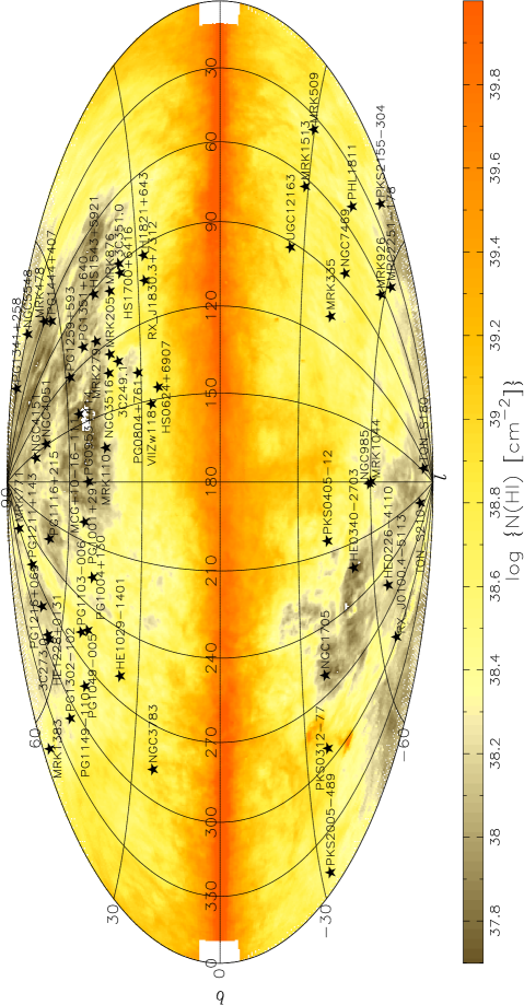
Figure 1: All-sky map of $N$(H I) integrated between $-$100 and 100 km s^-1, using the Leiden-Argentina Bonn survey (Kalberla et al. 2005), with the column density scale on the bottom. The directions to our 59 targets are shown by the stars and labels.

Table 1: Observational data

Object	Lon	Lat	Type	Obs. ID.	Grating	$\lambda_{\rm min}$	$\lambda_{\rm max}$	Texp	GBT
	[∘]	[∘]				[Å]	[Å]	[ks]
(1)	(2)	(3)	(4)	(5)	(6)	(7)	(8)	(9)	(10)
3C249.1	130.39	38.55	QSO	O6E1/24$-$30	E140M	1140	1729	68.8	Y
3C273.0	289.95	64.36	QSO	O5D3/01$-$02	E140M	1140	1709	18.7	Y
3C351.0	90.08	36.38	QSO	O579/01$-$04	E140M	1140	1709	77.0	Y
H1821+643	94.00	27.42	QSO	O5E7/03$-$05	E140M	1140	1709	50.9	Y
HE0226$-$4110	253.94	-65.77	QSO	O6E1/07-11	E140M	1143	1729	43.8
HE0340$-$2703	222.68	-52.12	QSO	O8EI/03	G140M	1194	1250	4.9
HE1029$-$1401	259.33	36.52	QSO	O4EC/05	G140M	1194	1248	4.1
HE1228+0131	291.26	63.66	QSO	O56A/01$-$02	E140M	1140	1729	27.2
HS0624+6907	145.71	23.35	QSO	O6E1/12$-$16	E140M	1140	1729	62.0	Y
HS1543+5921	92.40	46.36	QSO	O8MR/01	G140M	1194	1250	25.3
HS1700+6416	94.40	36.16	QSO	O4SI/01$-$05	E140M	1140	1729	99.4
MCG+10$-$16-111	144.21	55.08	Sey	O5EW/02	G140M	1194	1249	19.5	Y
MRC2251$-$178	46.20	-61.33	QSO	O4EC/03	G140M	1194	1249	6.0	Y
Mrk110	165.01	44.36	Sey	O4N3/52	G140M	1194	1249	2.2	Y
Mrk205	125.45	41.67	Sey	O62Q/03$-$05	E140M	1140	1729	62.1	Y
Mrk279	115.04	46.86	Sey	O6JM/01	E140M	1140	1709	13.2
				O8K1/01$-$05	E140M	1140	1709	52.8
Mrk335	108.76	$-$41.42	Sey	O8N5/04-05	E140M	1140	1729	15.2	Y
Mrk478	59.24	65.03	Sey	O4EC/14	G140M	1194	1249	7.6	Y
Mrk509	35.97	$-$29.86	Sey	O6AP/01	E140M	1140	1709	7.6	Y
Mrk771	269.44	81.74	Sey	O4N3/05	G140M	1194	1249	2.0	Y
				O4EC/07	G140M	1194	1249	5.8
Mrk876	98.27	40.38	Sey	O8NN/01$-$02	E140M	1140	1729	29.2	Y
Mrk926	64.09	$-$58.76	Sey	O4EC/12	G140M	1194	1249	3.9
Mrk1044	179.69	$-$60.48	Sey	O8K4/01	G140M	1194	1250	2.4	Y
Mrk1383	349.22	55.13	Sey	O8PG/01$-$02	E140M	1140	1729	19.2	Y
Mrk1513	63.67	$-$29.07	Sey	O4EC/10	G140M	1194	1249	7.3	Y
NGC985	180.84	$-$59.49	Sey	O4EC/11	G140M	1194	1249	3.7	Y
NGC1705	261.08	$-$38.74	Sey	O58N/01-02	E140M	1140	1709	17.1
NGC3516	133.24	42.40	Sey	O57B/02	E140M	1140	1729	5.5
NGC3783	287.46	22.95	Sey	O57B/01	E140M	1140	1729	5.4
				O63M/01$-$17	E140M	1140	1729	87.0
				O63M/53	E140M	1140	1729	4.9
NGC4051	148.88	70.09	Sey	O5F0/01	E140M	1140	1729	10.3
NGC4151	155.08	75.06	Sey	O578/01	E140M	1140	1729	5.5
				O5KT/02,53,54	E140M	1140	1729	6.6
				O61L/01	E140M	1140	1729	9.4
				O6JB/01	E140M	1140	1729	7.6
NGC5548	31.96	70.50	Sey	O4LL/01	E140M	1140	1729	4.8	Y
				O6JD/01$-$02	E140M	1140	1729	15.3
				O6KW/01$-$04	E140M	1140	1729	52.2
NGC7469	83.10	$-$45.47	Sey	O6BN/01	E140M	1140	1729	13.0	Y
				O8N5/01$-$02	E140M	1140	1729	22.8
PG0804+761	138.28	31.03	QSO	O4N3/01	G140M	1194	1249	2.4	Y
				O4EC/06	G140M	1194	1249	4.9	Y
PG0953+414	179.79	51.71	QSO	O4X0/01$-$02	E140M	1140	1729	25.5	Y
PG1001+291	200.08	53.21	QSO	O6E1/17$-$23	E140M	1140	1729	48.4	Y
PG1004+130	225.12	49.12	QSO	O5EW/03	G140M	1194	1249	5.2
PG1049$-$005	252.28	49.88	QSO	O4N3/03	G140M	1194	1249	1.5
PG1103$-$006	256.66	52.30	QSO	O4N3/04	G140M	1194	1249	1.4
PG1116+215	223.36	68.21	QSO	O5A3/01$-$02	E140M	1139	1709	6.6
				O5E7/01$-$02	E140M	1140	1709	19.9
PG1149$-$110	280.47	48.89	Sey	O5EW/05	G140M	1194	1250	8.1
PG1211+143	267.55	74.31	Sey	O61Y/01$-$08	E140M	1140	1729	42.5	Y
PG1216+069	281.07	68.14	QSO	O6E1/31$-$39	E140M	1140	1729	69.8	Y
PG1259+593	120.56	58.05	QSO	O63G/05$-$11	E140M	1143	1729	95.8
PG1302$-$102	308.59	52.16	QSO	O5BU/01,02,61	E140M	1140	1729	22.1	Y
PG1341+258	28.71	78.15	QSO	O5EW/01	G140M	1194	1250	6.9	Y
PG1351+640	111.89	52.02	Sey	O4EC/54	G140M	1194	1248	14.7	Y
PG1444+407	69.90	62.72	QSO	O6E1/01$-$06	E140M	1140	1729	48.6	Y
PHL1811	47.47	$-$44.82	QSO	O8D9/01-04	E140M	1140	1729	33.9	Y
PKS0312$-$77	293.44	-37.55	QSO	O65T/01,02,13	E140M	1140	1729	8.4
PKS0405$-$12	204.93	-41.76	QSO	O55S/01,02	E140M	1139	1729	27.2	Y
PKS2005$-$489	350.37	-32.60	BLLac	O4EC/09	G140M	1194	1249	6.1
PKS2155$-$304	17.73	-52.25	BLLac	O5BY/01-02	E140M	1139	1729	28.5
RX J0100.4$-$5113	299.48	-65.84	Sey	O8P8/02	G140M	1194	1250	2.3
RX J1830.3+7312	104.04	27.40	Sey	O5EW/09	G140M	1194	1249	5.8	Y
Ton S180	139.00	$-$85.07	Sey	O4EC/02	G140M	1194	1249	4.1	Y
Ton S210	224.97	$-$83.16	QSO	O6L0/01-02	E140M	1140	1709	12.3
UGC12163	92.14	$-$25.34	Sey	O5IT/05	E140M	1140	1709	10.3
VIIZw118	151.36	25.99	Sey	O4EC/13	G140M	1194	1249	9.5	Y

Note. — Col. (1): Object name. Cols. (2,3): Galactic longitude and latitude. Col. (4): Object type; QSO is a quasar and Sey is a Seyfert galaxy. Col. (5): Observational program identification datasets with exposure identifications. Col. (6): Grating used for observation; either HST STIS$-$G140M or HST STIS$-$E140M. Cols. (7,8): Minimum and maximum wavelength of observational wavelength spanned. Col. (9): Total exposure time. Col. (10): “Y” means there is a spectrum taken with the Green Bank Telescope.

2 Observations

2.1 HST data

We used Hubble Space Telescope (HST) observations of AGNs that were observed at sufficient spectral resolution to (mostly) resolve the interstellar and intergalactic absorption lines. This includes observations using the G140M grating and E140M echelle in the Space Telescope Imaging Spectrograph (STIS). G140M spectra cover a wavelength interval about 55 Å wide at 30 km s^-1 resolution, while E140M spectra range from 1140 to 1710 Å with a resolution of 6.5 km s^-1. The calibrated HST data were retrieved from the Multimission Archive at STScI (MAST) server. We do not look at the many targets observed with the STIS-G140L grating, since the interstellar lines near 1200 and 1206 Å in the damping profile are not fully resolved in such low-resolution (300 km s^-1) data, nor are low-redshift intergalactic Ly$\alpha$ or high-redshift intergalactic metal lines. When unresolved, such lines change the apparent continuum, making it more difficult to obtain reliable results. We list the sample of 59 AGNs in Table 1. The locations of these targets on the sky are shown in Fig. 1.

2.2 Fitting Method

To measure $N$(H I), the continuum-reconstruction method was used, which works as follows. First, one assumes an H I column density and a linewidth, which yields an optical depth ($\tau$) profile. Multiplying the observed spectrum with $\exp(+\tau)$ then gives a “reconstructed” continuum, which is assumed to be smooth as well as continuous with the parts of the spectrum where the continuum is observed directly. The H I column density is then varied until this is actually the case. We now describe this in more detail.

Before applying this method, we first increased the signal to noise (S/N) ratio of the spectra by binning the E140M data by 15 pixels (to 48 km s^-1 or 7 resolution elements), and the G140M data by 3 pixels (to 40 km s^-1 or 1.3 resolution elements). Then we defined a continuum ($C$) by selecting regions free of absorption and emission in a window about 50 Å wide around the Ly$\alpha$ line and fitting a Legendre polynomial of order up to 4 through these selected points, using the method of Sembach & Savage (1992). To ensure the continuity and smoothness of the reconstructed continuum, some of these regions are placed so that the final fit is made through the reconstructed continuum in regions where there is Ly$\alpha$ absorption.

Next, we created a reconstructed continuum starting with the $N$(H I) value obtained from the 21-cm brightness temperature. The velocity of the H I profile was also determined from the 21-cm H I emission data toward the sightline (see Sect. 2.3 below). Using the velocity and column density, we multiplied the observed flux ($F$) by $\exp(+\tau)$, where $\tau$ is the optical depth of the Ly$\alpha$ line, including its damping wings. We note that the width of the central gaussian part of the absorption profile is not important for the shape of the damping wings.

Finally, we made a fit to the continuum by changing the column density value until the fitted continuum a) looked smooth and b) minimized the difference between the fit and the reconstruction. The minimization is done by calculating a reduced $\chi^{2}$ as:

$$\chi^{2}\ =\ {1\over n}\ \Sigma\left({C-F\ e^{\tau}\over\delta F\ e^{\tau}}\right)^{2},$$

where $C$ is the fit to the reconstucted continuum, $F$ is the observed flux, $\delta F$ is the error in the flux, and $n$ is the number of independent pixels. This calculation is only done in selected regions of the spectrum, which are different from those used to define the continuum. The selected regions are those that a) are within about 10 Å of the central wavelength of Ly$\alpha$ (1215.67 Å), b) are free of intergalactic or interstellar absorption lines, c) have the optical depth of the Ly$\alpha$ line $<$1.5, and d) have an S/N ratio ($F$/$\delta F$) $>$2. The range of $N$(H I) values at which $\chi^{2}$=$\chi^{2}_{\rm min}$+1 determines the error in each $N$(H I) result.

Some sightlines contain high-velocity H I components. In such cases, we applied a procedure to determine a systematic error in $N$(H I) for the low-velocity components. To do this, we systematically varied the column density of one component, while fitting the other. Specifically, for sightlines with a HVC having $N$(H I) between $\sim$2$\times 10^{19}$ and $10^{20}$ ${\rm cm^{-2}}$, we fixed $N$(H I; HVC) at the nominal 21-cm value, as well as at nominal$\times$1.5 and nominal/1.5, and then fitted the column density of the low-velocity component for each of these three HVC component values. The resulting range of $N$(H I) values for the low-velocity component then gave an estimate of the uncertainty associated with having the high-velocity component present. For sightlines containing high- and low-velocity components with similar strengths, the components were varied by 20% instead of 50%, since the result is better constrained in this case. We then executed the procedure of fixing one component and fitting the other for both components separately, while defining a region to calculate $\chi^{2}$ on only one side of the Ly$\alpha$ absorption line. In most of these case we decided in the end that the systematic error in the final values was too large to use the results in the analysis of column density ratios.

2.3 21-cm data

We used three sources of 21-cm data. For 35 of the targets that have Ly$\alpha$ spectra we obtained new data with the Green Bank Telescope (GBT) at an angular resolution of 9$\farcm$1 (see below for more details on these observations). In 167 directions (42 overlapping with the Ly$\alpha$ sample), we also used the spectra of Lockman & Savage (1995), which were taken with the Green Bank 140-ft (21′ beam). For each of the directions in the merged Ly$\alpha$+GBT+140′ list, we interpolated between the grid points of the Leiden-Argentina-Bonn survey (Kalberla et al. 2005), a whole-sky survey done at 1.3 km s^-1 velocity resolution with a 36′ beam on a 0$\fdg$5$\times$0$\fdg$5 grid. For each object, the 21-cm column density, $N$(H I; 21cm), was obtained by integrating the brightness temperature over a specified velocity interval and converting this to a column density using

$$N(H\,I)\ =\int\ 1.823\hbox{$\times 10^{18}$}\ T_{s}\ \ln\left({T_{s}\over T_{s}-T_{\rm B}}\right)\ dv.$$

We analyze the highest $T_{B}$ half of each spectrum with $T_{s}$=135K and the faintest $T_{B}$ half with $T_{s}$=5000 K and then add the two values.

This is justified by the fact that Heiles & Troland (2003) found that about 50% of the H I in the disk is “cold neutral medium” (CNM), with spin temperatures ranging from 30 K to several 100 K, with a median value of 70 K. The other half of the H I is “warm neutral medium” (WNM) with $T_{s}$$>$500 K. Our value of 135 K for the CNM is an average. We use the different possible values for $T_{s}$ to derive a systematic error (see below). For column densities below $10^{20}$ ${\rm cm^{-2}}$, the differences between assuming an optically thin cloud and $T_{s}$=70 K or $T_{s}$=135 K are $<$1.5%. Only above column densities of about 5$\times 10^{20}$ ${\rm cm^{-2}}$ (log $N$(H I)$>$20.7) does the difference become $>$5%. In our sample this only happens for sightlines toward which we compare 21-cm column densities derived with different radio telescopes, but not for sightlines where we measure Ly$\alpha$.

The total error on the column density was estimated by adding in quadrature four sources of error, one statistical and three systematic. First, for each spectrum the rms in the brightness temperature was calculated and converted to a corresponding error in column density for the velocity interval that the column density was integrated over. Second, a systematic error of 1$\times 10^{18}$ ${\rm cm^{-2}}$ due to baseline placement was assumed for LAB and GBT data. For the older Green Bank spectra this was set to 2$\times 10^{18}$ ${\rm cm^{-2}}$. In one case (3C 273.0) strong continuum emission in the beam results in a noticeably worse instrumental baseline. Therefore, we set the baseline error to 5$\times 10^{18}$ ${\rm cm^{-2}}$. Similar effects cause the baseline error for NGC 985 to be set to 2$\times 10^{18}$ ${\rm cm^{-2}}$. The third source of error is the stray radiation correction. Blagrave et al. (2010) and Boothroyd et al. (2011, in preparation) study the stray radiation effects for the GBT in detail and estimate that the stray radiation correction adds another 4 K km s^-1 of uncertainty to an H I profile, equivalent to 7$\times 10^{18}$ ${\rm cm^{-2}}$ in $N$(H I). However, this uncertainty only applies to the low-velocity emission near 0 km s^-1. Profile components in the H I spectrum that have velocities above about 50 km s^-1 are not affected as strongly, as there is much less bright emission elsewhere in the sky at those velocities. Therefore, for intermediate-velocity components ($v$$\sim$50 km s^-1) we used a systematic error associated with the stray radiation correction of 1$\times 10^{18}$ ${\rm cm^{-2}}$, while for high-velocity components ($v$$>$90 km s^-1) we set this error to zero. The final source of error is the assumed value for the spin temperature. We calculated $N$(H I) using the formula above with $T_{s}$ set to 70 K, with $T_{s}$=135 K, and using the optically-thin assumption (reducing the $T$ terms to $T_{B}$), and we took the rms variation between those three values as the corresponding error. The combined error is at most 0.04 dex (10%) for sightlines with log $N$(H I)$<$20.8, the highest value we find for a direction where Ly$\alpha$ is measured, but for the great majority of sightlines the combined systematic error is $<$5% and usually it is $<$2%.

Finally, we calculated the brightness-temperature weighted average velocity of the profile, which is used to center the absorption line model (see below). The velocity intervals were defined by visually determining the extent of the emission in each of the 21-cm spectra toward a target. In most cases the chosen interval was then set to be the same at each angular resolution, but in a few cases small adaptations were necessary. To compare the 21-cm emission to the Ly$\alpha$ absorption, the full extent of the H I emission was used, but high- and intermediate-velocity components were measured separately when comparing column densities between different 21-cm observations.

2.4 GBT data

Of the 59 AGNs with UV data, 35 were newly observed during 2008 and 2009, using the Green Bank Telescope (GBT) at 0.8 km s^-1 spectral resolution and 9$\farcm$1 angular resolution.

The calibration of the GBT data took advantage of a recent, extensive investigation into the all-sky response of the telescope at 21 cm, made by a group which includes one of us (FJL). The detailed results will be given in Boothroyd et al. (2011, in preparation) and are summarized in Blagrave et al. (2010). Because the calibration is critical to the Ly$\alpha$ vs 21 cm comparison, we give a short summary here. Note that the GBT 21-cm and UV calibrations are completely independent: information from the Ly$\alpha$ measurements was never used in the GBT calibration.

The GBT is unique among large single dishes in that it has a clear aperture and thus does not have the sidelobes caused by scattering from the feed support legs, subreflector, and other blockage in the aperture (Prestage et al. 2009). The only significant sidelobes arise from spillover past the primary and secondary reflectors. Thus the telescope response can, to a significant degree, be derived from theoretical calculations. Boothroyd et al. (2011, in preparation) used calculations to determine the telescope response near the main beam, and used observations of the Sun to determine the spillover sidelobes. The aperture efficiency was derived from an electromagnetic analysis of the telescope which incorporated the detailed telescope geometry and measured illumination pattern of the 21 cm receiver. The antenna temperature scale was then established using this efficiency and observations of the radio source 3C 286 whose absolute flux was taken from Ott et al. (1994). There is agreement between this antenna temperature scale and one derived from laboratory measurements of the receiver noise diodes to within 2.4%. The same calculations established the main beam efficiency as 0.88. Measurements of the moon (which fills the GBT beam) were made to check the accuracy of the main beam efficiency and of point-sources to check the calculated main beam shape. In both cases the observations agreed with the calculations to within a few percent.

The forward and rear spillover lobes were measured by mapping large areas around the Sun. Given knowledge of the amplitude and location of these sidelobes, the Leiden-Dwingeloo 21 cm H I survey (Hartmann & Burton 1997) was then used to estimate the “stray” component of 21 cm emission in the GBT data which was then removed from the observations. The GBT has very low near sidelobes (more than 30 dB below the main beam gain) so no correction is made for stray radiation arising within one degree of the main beam. The derived main-beam brightness temperatures were corrected for atmospheric extinction assuming a zenith opacity of 0.008%.

The GBT 21-cm spectra were reduced and calibrated without reference to standard H I directions because we felt that for the GBT it would be more accurate to derive the calibration from fundamental flux density references and a detailed understanding of the antenna. In addition, the H I brightness temperature toward the standard directions is known to vary significantly with the angular resolution of the antenna (Kalberla et al. 1982). Nonetheless, the standard direction S8 was observed four times on two consecutive days during our experiment, and examination of these data, which were calibrated and corrected for stray radiation identically to the AGN directions, gives useful information. The GBT values for both the peak line brightness temperature and the line integral of S8 are in excellent agreement with those given in Kalberla et al. (1982), being in the ratio 0.994$\pm$0.004 and 0.991$\pm$0.001 for the peak and integral, respectively. The uncertainties are 1$\sigma$ about the mean of the four observations. Kalberla et al (1982) concluded that when stray radiation is taken into account the principal H I calibration observations (Penzias et al 1970; Wrixon and Heiles 1972; Williams 1973) are in agreement to within about 3%. Thus our data reduction procedure appear to produce GBT H I spectra with an accurate brightness temperature scale, one that is consistent with other calibrations.

Each source was measured by the GBT at least twice, and several as many as four times. This allows us to estimate an error term based on the reproducibility of the results. The short-term reproducibility is derived from sequential scans; here the main sources of error should be noise and instrumental baseline changes. We find median short-term differences in the line integral of 0.4%, corresponding to median fluctuations in $N$(H I) of 1.1$\times 10^{18}$ ${\rm cm^{-2}}$. This is what would be expected from noise or baseline fluctuations already included in our error analysis.

Long term differences in spectra test not only baseline and gain stability, but the accuracy of the stray radiation correction. The median long-term uncertainty in the line integral is 2.3%, equivalent to $N$(H I)=1.9$\times 10^{18}$ ${\rm cm^{-2}}$. These differences lie well within that expected from uncertainty in the GBT stray radiation correction.

All of the tests that we have been able to make indicate that our fundamental calibration of the GBT H I spectra is accurate, and that our error estimates give a faithful representation of the uncertainties. At no time during this experiment, or during others that have measured many $10^{4}$ H I spectra with the GBT (e.g. Lockman et al. 2008), have 10% fluctuations in the GBT H I intensity scale been observed like those reported by Robishaw & Heiles (2009).

3 Systematic effects in the H I data

In this section we discuss the comparison between the column densities measured using Ly$\alpha$ absorption and 21-cm emission. A straightforward comparison between the values of $N$(H I) measured from 21-cm emission with those measured using various radio telescopes reveals significant differences between the two. In particular, for our set of low-column density directions, the values found with the Green Bank 140-ft and from the LAB survey are on average about 10% larger than those derived from Ly$\alpha$. On the other hand, no significant difference is found when comparing GBT and Ly$\alpha$ column densities. Below we will show why we think that these differences arise from the presence of a broad, spurious component in the LAB and 140-ft spectra. The amplitude and FWHM of this component are 0.048 K and 167 km s^-1 for LAB spectra, 0.023 K and 134 km s^-1 for 140-ft data with 2 km s^-1 channels, and 0.12 K and 70 km s^-1 for 140-ft data with 1 km s^-1 channels, corresponding to column densities of 15.3$\times 10^{18}$, 5.9$\times 10^{18}$ and 15.8$\times 10^{18}$ ${\rm cm^{-2}}$.

We discovered this after our referee pointed us to a website commonly used to obtain column densities from the LAB data (http://heasarc.gsfc.nasa.gov/cgi-bin/Tools/w3nh/w3nh.pl). Although this helped us to figure out the problems, we want to point out that we have concluded that this website gives incorrect answers. In particular, it gives column densities that are derived after interpolating between the pixels of a gridded all-sky map smoothed (by default) to a one degree beam. Thus, a varying number of original LAB spectra is used to derive a column density. When using half a degree as the smoothing radius there are directions where the website says that there are no data on positions where an actual observation was done. Furthermore, in most cases the column density that it gives for a position where an actual spectrum was taken differs from the column density derived from that actual spectrum.

However, comparing our numbers with those given by this website led us to the realization that integrating LAB spectra from $-$400 to 400 km s^-1 gives different results than integrating over the line core, i.e., the velocity range where emission appears present. We had done the latter, in order to increase the S/N ratio by avoiding integrating over a 300 km s^-1 window containing only noise, as well as to be able to separate out high-velocity emission. For the LAB spectra, the two different integrals differ by a constant offset of $\sim$6$\times 10^{18}$ ${\rm cm^{-2}}$, as shown in Fig. 2. Since the highest H I column density in the set of sightlines with Ly$\alpha$ data is only about 7$\times 10^{20}$ ${\rm cm^{-2}}$, we added 90 sightlines with higher column density to make this comparison. These 90 sightlines were chosen at latitudes $b$=0^∘ to $b$=30^∘, at longitudes 170^∘, 180^∘ and 190^∘. This extends the comparison to $N$(H I)$\sim$7$\times 10^{21}$ ${\rm cm^{-2}}$.

The origin of the offset seen in Fig. 2 becomes clear if we examine the parts of the 21-cm spectra outside the bright line cores. Figure 3 shows the resulting averages of the non-signal regions of each spectrum. That is, for each direction we selected the channels outside the velocity limits given in Table 2. These limits are based on visually inspecting the spectra and selecting the velocity range where emission appears present. We did this for the GBT, 140-ft and LAB spectra in the same set of directions. Panel (a) gives the residual spectrum for the combined set of all LAB directions (i.e., the those with Ly$\alpha$, GBT and 140-ft, as well as the higher column densities directions used to make Fig. 2). Panels (d), (e) and (f) show the residuals for the two kinds of 140-ft spectra (with 2 km s^-1 and 1 km s^-1 channel spacing), and for the GBT spectra. Further, in panels (b) and (c) we show the residual LAB spectra for the directions corresponding to the 140-ft and the GBT sightlines. Gaussians were fit to the resulting features in order to determine the total emission in this broad component. Note that the GBT data show no significant broad component, although we show the formal fit.

Figure 2: Comparison between column densities derived from LAB spectra when integrating from $-$400 to 400 km s^-1 ($N$(H I)($-$400:400)) to values derived when integrating only over the region where emission is visible ($N$(H I)(em)). Red points are for the directions toward the AGNs for which we analyzed Ly$\alpha$ spectra. Black points are for higher-column density directions along three strips at $l$=170^∘, 180^∘ and 190^∘, $b$=0^∘ to 30^∘, in steps of 1^∘. A least squares-fit to these differences gives a slope of zero and an offset of 0.65$\times 10^{18}$ ${\rm cm^{-2}}$.

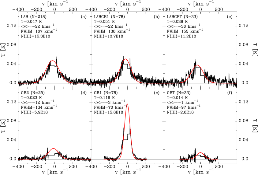
Figure 3: Black lines show the residual spectra for LAB, Green Bank 140-ft and GBT data, created by cutting out the region in each individual spectrum where H I emission is visually present. Panel (a) is for LAB spectra in the combined set of directions formed by our GBT, 140-ft spectra and the two strips near $l$=180^∘ used to create Fig. 2. Panels (d) and (e) are for 140-ft spectra, with panel (d) for spectra having 2 km s^-1 channel spacing and panel (e) for spectra with 1 km s^-1 channels. Panel (b) shows the LAB residual for the 140-ft directions. Panel (f) is the residual for the GBT spectra, while panel (c) is the LAB residual for the GBT directions. The red lines are gaussian fits to the residuals, with the parameters of the gaussian given in the label near the top of each panel. The label also gives the number of spectra used to make these residuals (N=#), and the integrated column density corresponding to the gaussian.

The broad residual component in the LAB spectra has a FWHM of 167 km s^-1 (dispersion 71 km s^-1) and a column density of 1.5$\times 10^{19}$ ${\rm cm^{-2}}$. We note that a similar broad underlying component in the LAB spectra was originally found by Kalberla et al. (1998), who measured a component with dispersion 60 km s^-1 (FWHM 140 km s^-1) and total column density 1.4$\times 10^{19}$${\rm cm^{-2}}$. Kalberla et al. (1998) interpreted this as evidence for a halo component in the Galactic H I, with scaleheight 4.4 kpc. However, we will now show that the overwhelming preponderance of evidence points to the conclusion that this broad underlying component is an artifact. This is based on the following four arguments.

(1) There is no residual component in GBT spectra. Since theoretically the GBT has very stable baselines, and is less affected by stray radiation than the LAB dataset, we weigh the absence of a residual in the GBT spectra as an argument in favor of the conclusion that the residual seen in the LAB spectra is an artifact.

(2) The residual emission seen in LAB and 140-ft spectra differs. Where the LAB spectra produce a residual feature that is a gaussian with $T$=0.048 K and FWHM=167 km s^-1, the 140-ft data with 2 km s^-1 channels give a gaussian with $T$=0.023 K, FWHM=134 km s^-1. Notably, 140-ft with 1 km s^-1 channel spacing give $T$=0.12 K, FWHM=70 km s^-1. Thus, the width of the gaussian differs for the two sets of similarly-calibrated but differently-setup 140-ft data, even though the same velocity ranges in the same spectra were used to create these residuals. Further, both residuals differ from that in the LAB data. This again suggests that the residual emission is an artifact. Still, it is possible that the calibration of the LAB spectra was better and the broad component is only properly picked up in that dataset. On the other hand, the difference in residual between the two kinds of 140-ft data suggests that it may be caused by a (small) baseline fitting error.

(3) The broad component produces no metal-line absorption. If there is a broad H I component in the Galaxy, this should result in a detectable optical depth for many ionic absorption lines in the ultraviolet. For instance, for solar metallicity gas with typical dust content, a component with FWHM 170 km s^-1 will produce a peak optical depth of $>2$ in the C II$\ \lambda\lambda$1334.532, 1036.337, O I $\lambda$1302.169 and Si II $\lambda$1260.422 lines. This would yield a dark line out to $\pm$150 km s^-1 in every sightline. As can be seen from the spectra toward 100 AGNs presented by Wakker et al. (2003), this is clearly not observed. A typical example for a direction without any known 21-cm emitting high-velocity gas is shown in Fig. 4. In fact, in all directions the extent of the strong metal lines is rather similar to the visual extent of the H I emission. Figure 4 also includes the absorption profile that would be associated with the high-dispersion gas if it had 1/10th solar metallicity. This could be the case if the high-dispersion gas consisted of infalling gas. However, in that case there would still be clear extended wings, which are also not observed. Thus, if this high-dispersion component were Galactic gas, there would be unmistakeable evidence for it in these spectra, unless its metallicity is much less than 0.1 times solar.

Figure 4: A typical example of the observed C II $\lambda$1334.532 absorption line compared to the expected absorption if there were high-dispersion material in the H I profile with FWHM 167 km s^-1 and $T_{B}$=0.048 K. Two smooth theoretical curves are shown on top of the data, one for solar metallicity (going down to having no flux in the center) and one for 1/10th solar metallicity. In neither case are the broad wings expected from a high velocity-dispersion interstellar component seen in the actual C II line.

(4) The broad component can not originate as an average of a population of small clouds. The only way in which a broad component might be absent in absorption line spectra, is if it consists of many small clumps, which are missed in all of the 100 or so observed AGN sightlines. Since 100 sightlines were sampled, to have a 50–50 probability of missing the small clouds in all sightlines requires that they have an area covering fraction of $<$0.7%, since 0.993¹⁰⁰=0.5. To have one such cloud in every 0$\fdg$5 beam thus requires clouds with diameters that are less than 3′. As the observed brightness temperature at 36′ resolution is 0.048 K, this implies an actual brightness temperature of 7 K, which for clouds with linewidth 15 km s^-1 would imply a colum density of 2$\times 10^{20}$. When observed with a 10′ beam, these clouds would have apparent brightness temperatures of 0.6 K and apparent column densities of $10^{19}$ ${\rm cm^{-2}}$. The population should have a cloud-to-cloud dispersion of 70 km s^-1, and be widespread at low and high latitudes.

A population of small clouds has indeed been discovered (Lockman 2002; Ford et al. 2008, 2010). These studies find 400 and 255 small clouds in two 720 square degree regions (0.45 per square degree), with the clouds having typical peak brightness temperature 0.5 K, typical velocity width 13 km s^-1, and typical size 20′ (i.e. many are unresolved). However, although the brightness temperature of these clouds is similar to what is required, they are much too large, the population strongly is confined to low latitudes, and the cloud-to-cloud dispersion is only 16 km s^-1. Thus, these clouds do not fit the requirements, and the observations show that a population of clouds with the required characteristics to mimic the broad component in the LAB spectra does not exist.

Combining points (1) through (4) leads to the conclusion that the residual emission in the LAB spectra is an artifact. The residual could be due to a final imperfection in the stray radiation correction. It might also be caused by a small error in the polynomials used to fit the baselines. Such an error would be difficult to discern since the largest visible deviation is $\sim$0.02 K, or less than 1/3rd the rms noise in a single spectrum. The fact that the spectra from different telescopes have different residuals argues for the second option. The fact that no significant residual is seen in the GBT spectra argues that the first option might also play a role.

Based on these considerations, we decided to correct the LAB and the 140-ft spectra, subtracting the gaussians shown in Fig. 3. This eliminates the discrepancies between the column densities derived from Ly$\alpha$ and those derived from 21-cm observations. As we show in the next section, the average ratio $N$(H I; Ly$\alpha$)/$N$(H I; 21cm) then becomes 0.96–1.00, with a dispersion of $\sim$0.10, not significantly different from 1. Without this correction, the average ratio is 0.90$\pm$0.10 for the LAB data and the LAB spectra are in tension with the Ly$\alpha$ column densities, with the GBT spectra, with the non-detection of metal-line absorption and with the observed population of small clouds. However, after applying the corrections, all tension between the many different observations disappears. In the remainder of the paper, we will thus only use corrected LAB and 140-ft column densities. We leave the GBT column densities uncorrected because there is no strong evidence that a correction is needed.

We also note the following. In Sect. 2.4 we had said that for the standard field S8 comparing the column density derived from the GBT data to that derived from the LAB survey gave a ratio of 0.991. The actual LAB column density toward S8 is 1.805$\times 10^{21}$ ${\rm cm^{-2}}$. Subtracting the spurious 1.5$\times 10^{19}$ ${\rm cm^{-2}}$ from this gives a column density of 1.790$\times 10^{21}$ ${\rm cm^{-2}}$. The ratio of these two values is 0.992. Thus, after correcting the LAB data, they give exactly the same column density as the GBT data in this direction.

4 Results

4.1 21-cm and UV data

In Fig. 5 we show the 21-cm and UV spectra of all AGN targets toward which we measured $N$(H I; Ly$\alpha$). The 21-cm spectrum that is displayed is the one obtained with the smallest telescope beam. In the panels with the UV spectra, we show the observed flux as well as the fitted continua and resulting models. The H I column densities derived from the 21-cm and Ly$\alpha$ absorption are shown for comparison. Table 2 presents a more detailed summary of the results, giving the UV column densities, as well as the 21-cm column densities obtained with different telescopes (see Sect. 2).

The spectra of targets observed with the STIS-G140M grating sometimes show a rise on the short-wavelength side of the spectrum, below 1200 Å. We have been unable to determine the origin of this spectral slope, but it may be due to a calibration error in G140M observations. The targets that show this effect are: Mrk 1044, Mrk 1513, PG 0804+761, PG 1049$-$005, PG 1341+258, PKS 2005$-$489, RX J0100.4$-$5113, RX J1830.3+7312, Ton S180, and VII Zw118, as can be seen in Fig. 5. Where possible, we avoided fitting the continuum using pixels below 1200 Å.

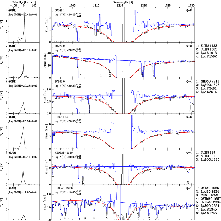
Figure 5a: Left: 21-cm brightness temperature versus LSR velocity in either Leiden-Argentina-Bonn survey, Green Bank 140-ft, or Green Bank Telescope (GBT) observations, as shown by the labels LAB, GB, and GBT. The available spectrum with the smallest beam on the sky is shown. The second label line gives log $N$(H I; 21cm) for each sightline. Right: Black histograms give the Ly$\alpha$ flux versus wavelength from HST STIS-G140M and STIS-E140M data. The blue histograms represent the flux after correction for the Galactic Ly$\alpha$ absorption. The smooth lines through the blue histograms are the reconstructed continua, which were fitted through the corrected data; see Sect. 2.2 for a complete description. The solid red lines give the final model fits to the data. The fits are calculated using the reconstructed continuum and the value of $N$(H I; Ly$\alpha$) that is listed in the label on the left. The quality factor for each sightline (see Sect. 4.3) is given in the label on the right. The dashed line at the bottom of each spectrum represents the error in the observed fluxes. For selected sightlines IGM or ISM emission or absorption lines are identified to the right of the spectra with corresponding numbers placed below the spectra and the heliocentric velocity of the line included in the label.

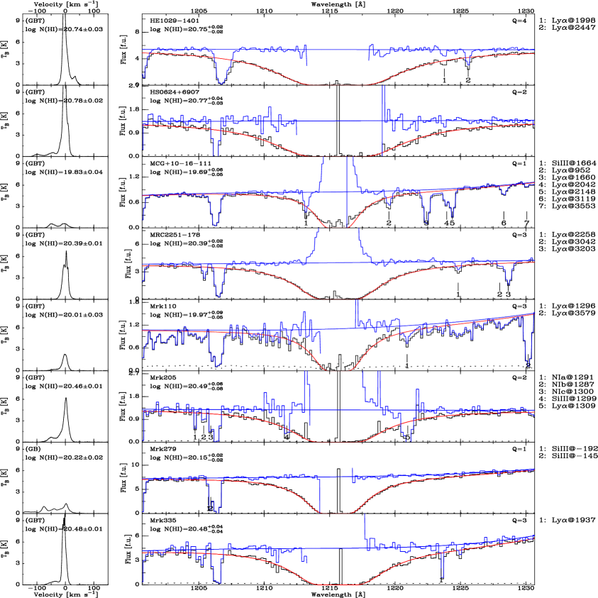
Figure 5b: Continued.

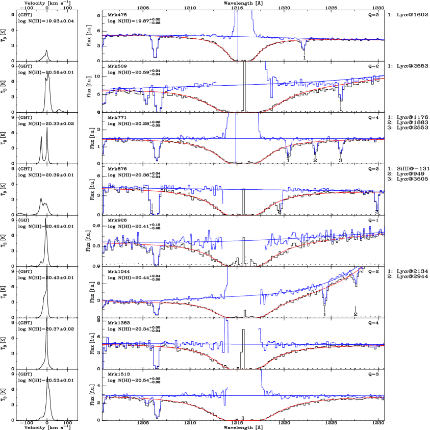
Figure 5c: Continued.

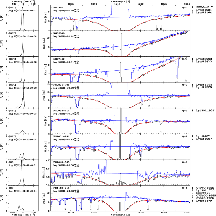
Figure 5d: Continued.

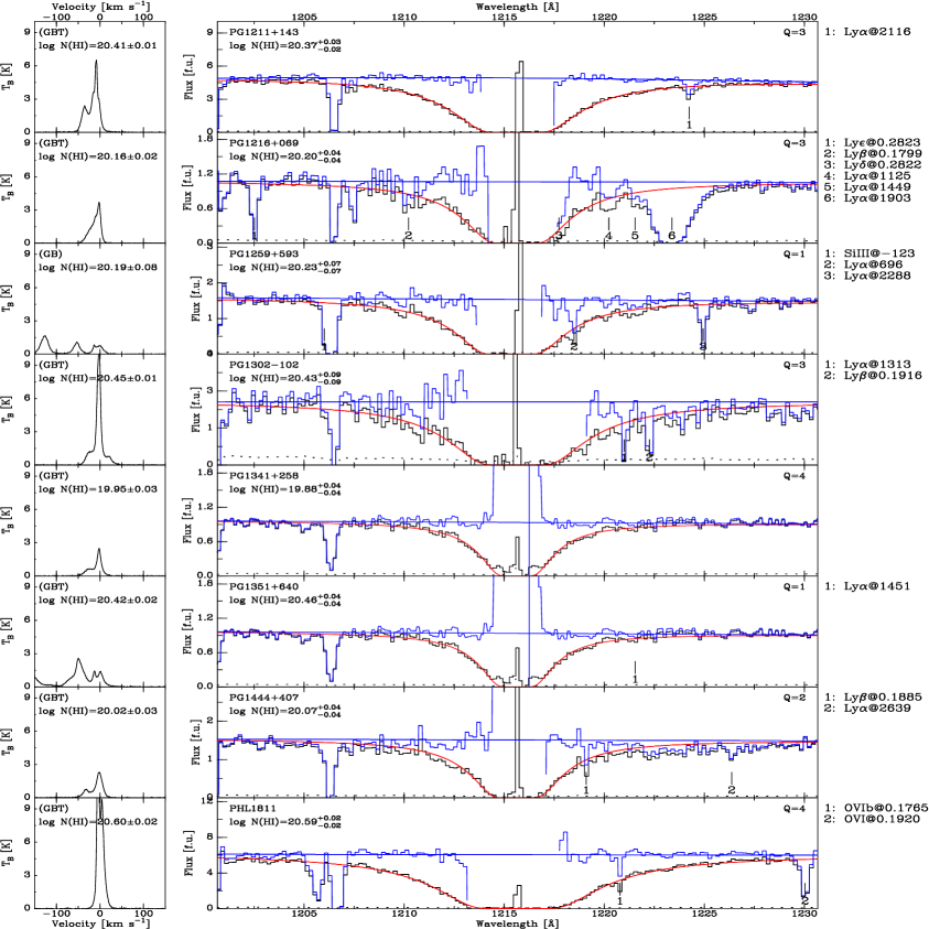
Figure 5e: Continued.

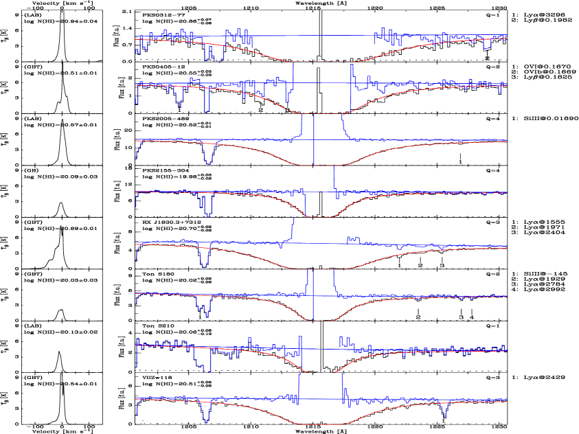
Figure 5f: Continued.

Table 2: Results

Object	Lon	Lat	Qual	log($N$(HI))	$N$(HI)(fixed)	$v_{\rm min}$	$v_{\rm max}$	$N$(HI)	$<v>$	$N$(HI)	$<v>$	$N$(HI)	$<v>$
	[∘]	[∘]		[${\rm cm^{-2}}$]	[$10^{18}$ ${\rm cm^{-2}}$	[km s-1]	[km s-1]	[${\rm cm^{-2}}$]	[km s-1]	[${\rm cm^{-2}}$]	[km s-1]	[${\rm cm^{-2}}$]	[km s-1]
				(Ly$\alpha$)	@km s-1]			(LAB)		(GB)		(GBT)
(1)	(2)	(3)	(4)	(5)	(6)	(7)	(8)	(9)	(10)	(11)	(12)	(13)	(14)
3C249.1	130.39	38.55	2	20.46${}_{-0.04}^{+0.03}$		$-$90	35	20.400$\pm$0.013	$-$11	20.431$\pm$0.013	$-$11	20.414$\pm$0.013	$-$9
3C273.0	289.95	64.36	2	20.25${}_{-0.02}^{+0.02}$		$-$55	50	20.169$\pm$0.026	$-$8	20.184$\pm$0.021	$-$4	20.108$\pm$0.032	$-$4
3C351.0	90.08	36.38	4	20.25${}_{-0.03}^{+0.03}$		$-$170	40	20.220$\pm$0.019	$-$10			20.226$\pm$0.018	$-$11
H1821+643	94.00	27.42	3	20.50${}_{-0.02}^{+0.02}$		$-$150	40	20.528$\pm$0.012	$-$12			20.536$\pm$0.011	$-$14
HE0226$-$4110a	253.94	$-$65.77	4	20.09${}_{-0.04}^{+0.03}$		$-$75	60	20.171$\pm$0.021	$-$6
HE0340$-$2703	222.68	$-$52.12	1	19.80${}_{-0.08}^{+0.08}$		$-$50	30	19.848$\pm$0.042	$-$2
HE1029$-$1401	259.33	36.52	4	20.75${}_{-0.02}^{+0.02}$		$-$45	100	20.740$\pm$0.030		20.757$\pm$0.028	1	20.736$\pm$0.029
HS0624+6907	145.71	23.35	2	20.77${}_{-0.03}^{+0.04}$		$-$125	50	20.791$\pm$0.025	$-$8			20.781$\pm$0.024	$-$7
MCG+10$-$16$-$111	144.21	55.08	1	19.84${}_{-0.04}^{+0.04}$		$-$120	50	19.736$\pm$0.056	$-$20			19.830$\pm$0.043	$-$24
	0.00	0.00	0	19.69${}_{-0.05}^{+0.06}$	20@$-$47	$-$25	50	19.498$\pm$0.093	$-$1			19.552$\pm$0.079	$-$1
	0.00	0.00	0	19.62${}_{-0.06}^{+0.06}$	26@$-$47
	0.00	0.00	0	19.53${}_{-0.08}^{+0.09}$	32@$-$47
	0.00	0.00	0	19.53${}_{-0.05}^{+0.08}$	31@$-$1	$-$120	$-$25	19.361$\pm$0.123	$-$45			19.505$\pm$0.087	$-$49
	0.00	0.00	0	19.45${}_{-0.07}^{+0.07}$	39@$-$1
	0.00	0.00	0	19.34${}_{-0.09}^{+0.09}$	47@$-$1
MRC2251$-$178	46.20	$-$61.33	3	20.39${}_{-0.02}^{+0.02}$		$-$50	50	20.374$\pm$0.015	$-$2	20.415$\pm$0.016		20.390$\pm$0.014
Mrk110	165.01	44.36	3	19.97${}_{-0.05}^{+0.09}$		$-$85	60	20.063$\pm$0.027	$-$6	20.056$\pm$0.027	$-$2	20.010$\pm$0.029	$-$6
Mrk205	125.45	41.67	2	20.49${}_{-0.08}^{+0.06}$	0@$-$199	$-$225	50	20.436$\pm$0.012	$-$24			20.463$\pm$0.012	$-$18
	0.00	0.00	0	20.48${}_{-0.08}^{+0.06}$	8@$-$199
	0.00	0.00	0	20.47${}_{-0.08}^{+0.06}$	16@$-$199
	0.00	0.00	0	20.46${}_{-0.09}^{+0.06}$	24@$-$199
Mrk279	115.04	46.86	1	20.15${}_{-0.02}^{+0.02}$		$-$175	40	20.128$\pm$0.023	$-$42	20.216$\pm$0.019	$-$44
Mrk335	108.76	$-$41.42	3	20.48${}_{-0.04}^{+0.04}$		$-$100	25	20.496$\pm$0.016	$-$8	20.555$\pm$0.015	$-$10	20.477$\pm$0.015	$-$7
Mrk478	59.24	65.03	2	19.87${}_{-0.02}^{+0.02}$		$-$75	50	19.916$\pm$0.037	$-$9	19.913$\pm$0.040	$-$6	19.927$\pm$0.035	$-$9
Mrk509	35.97	$-$29.86	2	20.59${}_{-0.04}^{+0.04}$		$-$60	105	20.613$\pm$0.013	7	20.617$\pm$0.013	6	20.583$\pm$0.012	8
Mrk771	269.44	81.74	4	20.28${}_{-0.03}^{+0.02}$		$-$60	60	20.415$\pm$0.016	$-$11	20.357$\pm$0.016	$-$11	20.327$\pm$0.016	$-$13
Mrk876	98.27	40.38	2	20.36${}_{-0.04}^{+0.04}$	0@$-$139	$-$210	60	20.346$\pm$0.015	$-$25	20.424$\pm$0.013	$-$32	20.395$\pm$0.015	$-$32
	0.00	0.00	0	20.34${}_{-0.05}^{+0.03}$	12@$-$139
	0.00	0.00	0	20.29${}_{-0.04}^{+0.05}$	25@$-$139
	0.00	0.00	0	20.26${}_{-0.04}^{+0.06}$	37@$-$139
Mrk926	64.09	$-$58.76	1	20.41${}_{-0.08}^{+0.15}$		$-$95	60	20.413$\pm$0.015	$-$6	20.417$\pm$0.015	$-$8
Mrk1044	179.69	$-$60.48	2	20.44${}_{-0.05}^{+0.04}$		$-$65	40	20.471$\pm$0.014	$-$8	20.452$\pm$0.014	$-$8	20.434$\pm$0.014	$-$7
Mrk1383	349.22	55.13	4	20.34${}_{-0.04}^{+0.05}$		$-$65	40	20.387$\pm$0.017	$-$5	20.382$\pm$0.017	$-$4	20.370$\pm$0.017	$-$3
Mrk1513	63.67	$-$29.07	3	20.54${}_{-0.02}^{+0.02}$		$-$75	50	20.550$\pm$0.013	2	20.544$\pm$0.013	3	20.534$\pm$0.013	3
NGC985	180.84	$-$59.49	3	20.50${}_{-0.04}^{+0.04}$		$-$50	50	20.537$\pm$0.015	$-$8	20.546$\pm$0.014	$-$6	20.534$\pm$0.015	$-$7
NGC5548	31.96	70.50	3	20.12${}_{-0.02}^{+0.03}$		$-$75	35	20.131$\pm$0.024	$-$7	20.172$\pm$0.022	$-$6	20.164$\pm$0.021	$-$8
NGC7469	83.10	$-$45.47	3	20.61${}_{-0.04}^{+0.06}$		$-$70	50	20.654$\pm$0.023	$-$4	20.643$\pm$0.021	$-$3	20.637$\pm$0.022	$-$3
PG0804+761	138.28	31.03	3	20.53${}_{-0.03}^{+0.03}$		$-$100	50	20.497$\pm$0.016	$-$6	20.525$\pm$0.016	$-$6	20.514$\pm$0.017	$-$5
PG0953+414	179.79	51.71	3	20.03${}_{-0.03}^{+0.03}$		$-$100	45	19.997$\pm$0.031	$-$14	20.039$\pm$0.028	$-$10	19.995$\pm$0.030	$-$12
PG1001+291	200.08	53.21	2	20.23${}_{-0.04}^{+0.04}$		$-$90	35	20.203$\pm$0.020	$-$24	20.210$\pm$0.019	$-$22	20.195$\pm$0.019	$-$22
PG1049$-$005	252.28	49.88	1	20.68${}_{-0.03}^{+0.03}$		$-$70	35	20.584$\pm$0.014	$-$13	20.616$\pm$0.015	$-$12
PG1116+215	223.36	68.21	1	19.85${}_{-0.05}^{+0.04}$	41@$-$6	$-$75	$-$25	19.863$\pm$0.042	$-$41	19.867$\pm$0.041	$-$41
	0.00	0.00	0	19.78${}_{-0.05}^{+0.05}$	51@$-$6
	0.00	0.00	0	19.71${}_{-0.07}^{+0.05}$	61@$-$6
	0.00	0.00	0	19.75${}_{-0.05}^{+0.06}$	54@$-$42	$-$25	25	19.635$\pm$0.068	$-$6	19.679$\pm$0.062	$-$6
	0.00	0.00	0	19.64${}_{-0.07}^{+0.07}$	68@$-$42
	0.00	0.00	0	19.48${}_{-0.11}^{+0.09}$	82@$-$42
PG1211+143	267.55	74.31	3	20.37${}_{-0.02}^{+0.03}$		$-$65	35	20.413$\pm$0.013	$-$17	20.410$\pm$0.015	$-$17	20.413$\pm$0.013	$-$16
PG1216+069	281.07	68.14	3	20.20${}_{-0.04}^{+0.04}$		$-$55	35	20.173$\pm$0.021	$-$11	20.173$\pm$0.026	$-$11	20.163$\pm$0.021	$-$10
PG1259+593	120.56	58.05	1	19.75${}_{-0.04}^{+0.07}$	(b)	$-$30	20	19.437$\pm$0.104	$-$6	19.585$\pm$0.081	$-$4
	0.00	0.00	0	19.65${}_{-0.05}^{+0.10}$	(b)	$-$95	$-$30	19.415$\pm$0.109	$-$51	19.602$\pm$0.078	$-$54
	0.00	0.00	0	19.98${}_{-0.03}^{+0.04}$	(b)	$-$160	$-$95	19.631$\pm$0.070	$-$128	19.837$\pm$0.047	$-$127
PG1302$-$102	308.59	52.16	3	20.43${}_{-0.09}^{+0.09}$		$-$70	55	20.497$\pm$0.015	$-$4	20.485$\pm$0.014	$-$4	20.455$\pm$0.015	$-$3
PG1341+258	28.71	78.15	4	19.88${}_{-0.04}^{+0.04}$		$-$65	55	20.002$\pm$0.032	$-$9	19.961$\pm$0.034	$-$7	19.945$\pm$0.034	$-$9
PG1351+640	111.89	52.02	1	20.46${}_{-0.04}^{+0.04}$	0@$-$149	$-$200	50	20.301$\pm$0.023	$-$59	20.401$\pm$0.021	$-$62	20.419$\pm$0.022	$-$62
	0.00	0.00	0	20.39${}_{-0.03}^{+0.05}$	33@$-$149
	0.00	0.00	0	20.33${}_{-0.04}^{+0.05}$	66@$-$149
	0.00	0.00	0	20.26${}_{-0.06}^{+0.04}$	99@$-$149
PG1444+407	69.90	62.72	2	20.07${}_{-0.04}^{+0.04}$		$-$65	35	20.008$\pm$0.030	$-$10	20.037$\pm$0.028	$-$10	20.022$\pm$0.029	$-$9
PHL1811	47.47	$-$44.82	4	20.59${}_{-0.02}^{+0.02}$		$-$45	50	20.606$\pm$0.018				20.599$\pm$0.019
PKS0312$-$77	293.44	$-$37.55	1	20.86${}_{-0.06}^{+0.07}$		$-$50	270	20.936$\pm$0.041	38
PKS0405$-$12	204.93	$-$41.76	2	20.55${}_{-0.03}^{+0.03}$		$-$45	40	20.508$\pm$0.012	1	20.531$\pm$0.014	3	20.509$\pm$0.013	3
PKS2005$-$489	350.37	$-$32.60	4	20.52${}_{-0.01}^{+0.01}$		$-$60	50	20.575$\pm$0.013	1
PKS2155$-$304	17.73	$-$52.25	4	19.98${}_{-0.02}^{+0.03}$		$-$55	55	20.117$\pm$0.024	$-$6	20.092$\pm$0.026	$-$4
RX J1830.3+7312	104.04	27.40	3	20.70${}_{-0.02}^{+0.02}$		$-$120	40	20.713$\pm$0.011	$-$15			20.692$\pm$0.010	$-$16
Ton S180	139.00	$-$85.07	2	20.02${}_{-0.02}^{+0.02}$		$-$120	30	20.104$\pm$0.025	$-$10	20.035$\pm$0.055	$-$6	20.031$\pm$0.028	$-$6
Ton S210	224.97	$-$83.16	1	20.06${}_{-0.13}^{+0.08}$		$-$50	30	20.129$\pm$0.023	$-$10
VIIZw118	151.36	25.99	3	20.51${}_{-0.02}^{+0.02}$		$-$75	50	20.543$\pm$0.014	$-$3	20.564$\pm$0.015	$-$3	20.539$\pm$0.015	$-$2

Note. — a: Savage et al. (2007) report log $N$(H I)=20.12$\pm$0.03 for this target. b: For PG 1259+593 three different components were held fixed. The table gives the fitted result for each of the three when using the nominal values for the other two. When varying the values for the components held fixed, the range in the derived value for the fitted component is about $\pm$0.10 dex for the HVC, $\pm$0.20 dex for the IVC and $\pm$0.05 dex for the LVC. Col. (1): Object name. Col. (2,3): Longitude, latitude. Col. (4): Quality factor; for complete description see Sect. 4. Col. (5): Logarithmic value of $N$(H I) derived using Ly$\alpha$, with error. Col. (6): $N$(H I) and velocity of component held constant for multiple-component spectrum fittings. See Sect. 2.2 for a complete description. Cols. (7,8): Velocity range over which the 21-cm profile was integrated to measure $N$(H I). Cols. (9)–(14): $N$(H I) derived from 21-cm data, and brightness-temperature weighted velocity of 21-cm cloud components from the Leiden-Argentina-Bonn, Green Bank 140-ft, and Green Bank Telescope (GBT) observations respectively.

4.2 Data Quality

Multiple factors contribute to the reliability of the fitted Ly$\alpha$ column densities, including the complexity of the 21-cm profile, noise in the UV spectrum, intrinsic AGN emission, galactic and intergalactic absorption lines, uncertainties in continuum placement, and the presence of multiple components. Each sightline was assigned a quality flag in the range of 0 to 4. These quality flags do not reflect the quality of the observations, but rather the reliability with which the column densities can be measured because of structure in the absorption and H I emission profiles. The nine quality four targets have flat continua with a high S/N ratio. The fifteen quality three targets are generally reliable but have potential problems with continua showing mild slope or curvature, weak emission and absorption lines, or multiple components in the 21-cm spectrum. The twelve quality two sightlines have moderately curved continua, moderate uncertainty in continuum placement, moderately strong emission and absorption lines, and multiple, well-separated 21-cm components of comparable strength. The ten quality one sightlines have low S/N, possibly high continuum curvature, strong intergalactic or intrinsic emission or absorption lines, or multiple 21-cm components. Finally, the thirteen quality zero targets have a significantly low S/N ratio, contain too many or too strong intrinsic emission or absorption lines, and multiple 21-cm components. We do not use the quality zero cases for the analysis. Generally, we do use quality one and two results, however, since it turns out that they do not change the properties of the distributions we calculate, but they do improve the statistics.

A quality factor between 0 and 4 was also assigned to each interstellar emission component in the LAB, GB 140-ft and GBT 21-cm profiles, based on the clarity and separation of the individual components of each profile. Many profiles contained additional intermediate- and high-velocity (IVC and HVC) components, which varied in their degree of separation from the low-velocity clouds (LVC). Quality four components either are a profile with a simple single-peak component or are components well-separated from other clouds in the same profile. Components that merge slightly with other clouds but are mostly separated were given quality three. Single-peak profiles with slightly extended tails were also rated as quality three. Quality two components either are clouds that show moderate blending with other clouds, or are components with a single-peak profile having broad extended tails, often containing fully merged IVC clouds. A quality factor of one was assigned for single-peak profiles that contain multiple IVC and/or HVC clouds that mostly blend together, Quality one was also given when the wings of clearly distinct IVC/HVC and/or LVC components blend with the wings and peaks of other components, but the components are clearly separate components.

In a few cases the profile was given quality zero. For instance, sometimes the spectrum shows emission at 0 and e.g. $-$40 km s^-1, but in one or more of the LAB, GBT, and/or GB 140-ft spectra these blend together, so that we no longer know how to calculate the associated column density for each. Or in one of the spectra there appears to be a weak IVC visible, which is not seen in another spectrum, either it is too small or because of noise. Most low-latitude ($b$$<$5^∘) sightlines were also given quality 0.

4.3 The 21-cm to Ly$\alpha$ column density ratio

In Fig. 6 we plot all combinations of log $N$(H I) derived using Ly$\alpha$, Leiden-Argentina-Bonn (LAB), Green Bank 140-ft (GB) and Green Bank Telescope (GBT) against each other. In Fig. 7 we show the ratios of these column densities. These figures show that although the values derived from the 21-cm and Ly$\alpha$ data are generally similar, they are not identical. Most of the low-column density points in the scatter plots for 21-cm-only data are values for the high-velocity clouds. Since the scatter clearly is larger for these clouds (red and blue points) than for the low-velocity gas (black points), they evidently have small-scale structure on scales of 9′–36′. The low-velocity components are possibly a mixture of clouds at different distances, each of which may have a column density similar to that of a HVC, as well as small-scale structure. However, all of these clouds get blended together in both the telescope beam and in the velocity-space of the sightline.

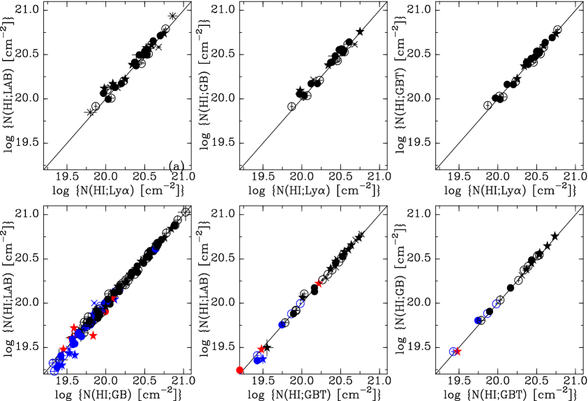
Figure 6: Plot comparing column densities derived using different telescopes. All combinations of log $N$(H I) derived from Ly$\alpha$, Leiden-Argentina-Bonn survey (LAB), the Green Bank 140-ft (GB) and the Green Bank Telescope (GBT) are plotted against each other. Closed stars are for measurements given quality 4, closed circles for quality 3, open circles for quality 2 and crosses for quality 1. Black symbols are for low-velocity gas, blue symbols for intermediate-velocity clouds and red symbols for high-velocity clouds.

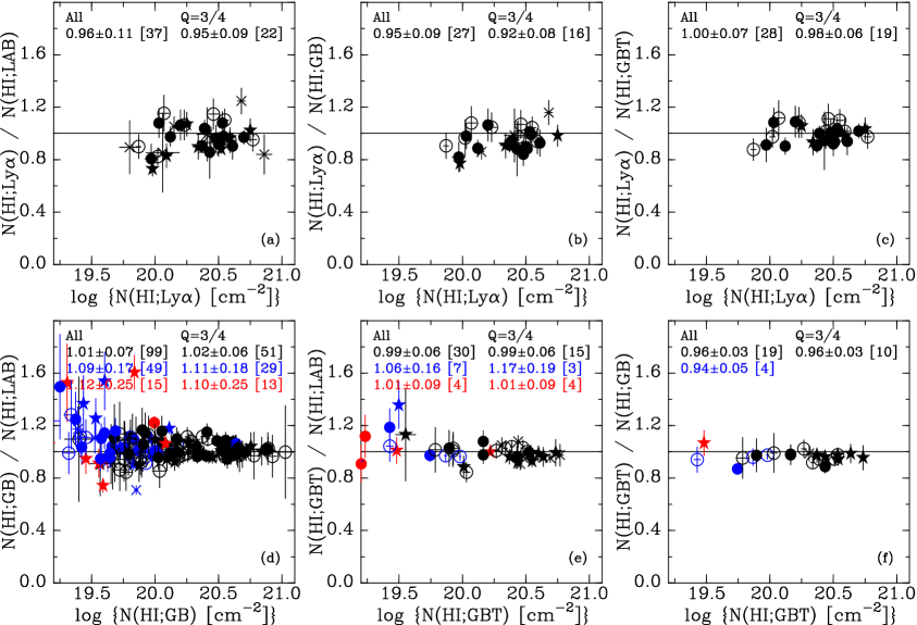
Figure 7: Plot showing the ratios of column densities derived using pairs of different telescopes against the column density of one of each pair. All combinations of log $N$(H I) derived from Ly$\alpha$, Leiden-Argentina-Bonn survey (LAB), the Green Bank 140-ft (GB) and the Green Bank Telescope (GBT) are plotted against each other. Closed stars are for measurements given quality 4, closed circles for quality 3, open circles for quality 2 and crosses for quality 1. Black symbols are for low-velocity gas, blue symbols for intermediate-velocity clouds, and red symbols for high-velocity clouds. In each of the panels the derived average ratio is shown using either all sightlines or only the Q=3/4 sightlines, separately for high-, intermediate- and low-velocity components, using the same color coding as for the symbols. In addition to the average ratio, we give an estimated error in that average (see text), as well as the number of sightlines used to derived the average, in square brackets.

In the ratio panels we also give the average ratio and its rms for all targets, and for targets with quality 3/4 only. Using LAB, GB and GBT data, on average, the ratios for all qualities are 0.96$\pm$0.11, 0.95$\pm$0.09 and 1.00$\pm$0.07, respectively. Using only the reliable (quality 3, 4) data, the 21-cm telescopes give average ratios of 0.95$\pm$0.09, 0.92$\pm$0.08 and 0.98$\pm$0.06, respectively. See Sect. 5.1 for further discussion of these ratios. Clearly, on average the ratio is slightly less than 1 in most cases, although not by much.

There are 22 sightlines for which we rated the Ly$\alpha$ measurement as high quality (3 or 4). For these datasets the ratio $N$(H I; Ly$\alpha$)/$N$(H I; LAB) ranges from 0.78 to 1.24, with the most extreme low ratio for toward PKS 2155$-$304, and the most extreme high toward PG 1049$-$005. For 16 sightlines with Q=3 or 4 and Green Bank 140-ft data the range is 0.77 to 1.16 (also for PKS 2155$-$304 and PG 1049$-$005). Nineteen sightlines with GBT data fall in the high-quality category, and the ratio of column densities ranges from 0.88 to 1.12 (Mrk 478 and PG 1444+407).

4.4 The 21-cm to 21-cm column density ratio

Figures 7d through 7f show the measurements of $N$(H I) when comparing different 21-cm telescopes against each other. LVC, IVC and HVC components are compared separately and are shown by black, blue and red symbols, respectively. These figures indicate that the different telescopes yield similar column densities for the low-velocity gas, which has column densities log $N$(H I)$>$19.4 to 21.0. The column densities of the IVC components span the column density range log $N$(H I)$\sim$18.6 to 20.2 (with one value near 20.6). The HVCs span a similar range as the IVCs, but cluster toward lower values. It is evident that the IVC and HVC column densities vary much more strongly between different 21-cm beams than the column densities of the low-velocity gas. It is likely that at least part of the reason for this is that the low-velocity emission originates from multiple clouds at different distances. Consequently, if it were possible to separate these clouds, the ratio of $N$(H I) derived from different telescopes would probably show a spread as large as that seen for the IVCs and HVCs.

Comparing the LAB, GB 140-ft and GBT data to each other shows that for high-quality low-velocity components, these three telescopes on average give the same value for $N$(H I) (average ratios of 1.01$\pm$0.07, 0.99$\pm$0.06 and 0.96$\pm$0.03, see labels in Fig. 7). The same is true for the intermediate- and high-velocity components, although the dispersions around the mean clearly are much larger in these cases. Also including the low-quality components increases the dispersions, but does not noticeably change the averages.

4.5 Comparison with FOS results

This paper was originally motivated by a desire to improve on the comparison between 21-cm and Ly$\alpha$ H I column densities using the measurements obtained with the FOS. In Table 3 we show the results of Savage et al. (2000) for the twelve sightlines that are in both samples. In Cols. 4 and 5 we compare the original 21-cm measurements with the ones we obtained here, showing the decrease due to correcting for the broad underlying spurious gaussian. Columns 2 and 3 give the Ly$\alpha$ column densities. All but one of our values are, on average, 15% (0.06 dex) larger than the ones obtained by Savage et al. (2000), as shown in Col. 6. This average excludes the factor two discrepancy for HS 0624+6907, whose FOS spectrum was difficult to measure, as is also shown by the fact that for this sightline the ratio $N$(H I; Ly$\alpha$)/$N$(H I; 21cm) was 0.46. With our new measurement, a more reasonable ratio of 0.97 is found.

For this set of sightlines, the ratio $N$(H I; Ly$\alpha$)/$N$(H I; 21cm) derived from the FOS data was 0.81$\pm$0.09, while with the new measurements it is 1.02$\pm$0.08.

Thus, where previously we found a large discrepancy in the average, now we find none. This is due to a combination of having much better UV data (increasing the derived $N$(H I; Ly$\alpha$) by 0.06 dex, which is less than the errors in the FOS measurements), and finding that the 140-ft data needed a correction (decreasing $N$(H I; 140’) on average by 0.05 dex). The change in the Ly$\alpha$ column densities is probably caused by the fact that for measuring the FOS spectra we needed to model and remove strong geocoronal emission, and the number of pixels to which the continuum could be fit was small. Nevertheless, the new values are all within the typical quoted error (0.2–0.3 dex) of the original ones. However, the correction in the 140-ft column densities is as important, and those corrections are larger than the errors in each individual measurement.

Table 3: Comparison between FOS and STIS measurements

Object	log($N$(HI))a	log($N$(HI))a	log($N$(HI))b	log($N$(HI))b	ratioc	ratioc	ratioc
	(Ly$\alpha$)	(Ly$\alpha$)	(GB)	(GB)	Ly$\alpha$/21-cm	Ly$\alpha$/21-cm	new/old
	[${\rm cm^{-2}}$]	[${\rm cm^{-2}}$]	[${\rm cm^{-2}}$]	[${\rm cm^{-2}}$]
	(FOS)	(STIS)	(old)	(new)	(old)	(new)
(1)	(2)	(3)	(4)	(5)	(6)	(7)	(8)
3C249.1	20.39${}_{-0.25}^{+0.25}$	20.46${}_{-0.04}^{+0.03}$	20.46	20.43	0.85	1.07	1.17
3C273.0	20.18${}_{-0.05}^{+0.05}$	20.25${}_{-0.02}^{+0.02}$	20.23	20.18	0.89	1.16	1.18
3C351.0	20.25${}_{-0.18}^{+0.52}$	20.25${}_{-0.03}^{+0.03}$	20.31	20.23	0.87	1.06	1.00
H1821+643	20.41${}_{-0.17}^{+0.19}$	20.50${}_{-0.02}^{+0.02}$	20.58	20.54	0.67	0.92	1.22
HS0624+6907	20.48${}_{-0.66}^{+0.48}$	20.77${}_{-0.03}^{+0.04}$	20.82	20.78	0.46	0.97	1.95
PG0953+414	19.92${}_{-0.05}^{+0.18}$	20.03${}_{-0.03}^{+0.03}$	20.05	20.04	0.74	0.98	1.29
PG1001+291	20.17${}_{-0.10}^{+0.17}$	20.23${}_{-0.04}^{+0.04}$	20.27	20.21	0.81	1.05	1.14
PG1116+215d	19.94${}_{-0.04}^{+0.04}$	20.05${}_{-0.05}^{+0.04}$	20.15	20.09	0.63	0.92	1.27
PG1216+069	20.11${}_{-0.07}^{+0.31}$	20.20${}_{-0.04}^{+0.04}$	20.19	20.17	0.83	1.06	1.22
PG1259+593d	20.13${}_{-0.07}^{+0.26}$	20.23${}_{-0.04}^{+0.07}$	20.19	20.19	0.88	1.11	1.26
PG1302-102	20.41${}_{-0.17}^{+0.19}$	20.43${}_{-0.09}^{+0.09}$	20.52	20.48	0.78	0.88	1.04
PKS0405-12	20.53${}_{-0.15}^{+0.34}$	20.55${}_{-0.03}^{+0.03}$	20.57	20.53	0.91	1.04	1.05

Note. — a: Cols. 2 and 3: column densities measured using Ly$\alpha$ data – values from Savage et al. (2000) based on FOS in Col. 2, values measured in this paper in Col. 3. b: Cols. 4 and 5: column densities measured using Green Bank 140-ft data – values from Savage et al. (2000) in Col. 4, values remeasured in this paper in Col. 5. c: Col. 6: ratio listed in Savage et al. (2000). Col. 7: improved ratio measured in this paper. Col. 8 gives the ratio between the old and new values. d: In these two sightlines there are multiple H I components with similar strengths. In the current paper we attempted to measure the Ly$\alpha$ column densities separately (see Sect. 4), while for the FOS data this was not done. Thus, the comparison between the FOS and STIS results is not as clear-cut as for the other sightlines.

5 Discussion

5.1 Does $N$(H I; Ly$\alpha$)/$N$(H I; 21cm) differ significantly from 1?

Table 4: Statistical test results

$N$(H I) source	Comp.	Qual	# points	$<$ratio$>$	$t$	$P$
(1)	(2)	(3)	(4)	(5)	(6)	(7)
Lya/LAB	TOT	All	37	0.96$\pm$0.15	1.64	5.51%
Lya/LAB	TOT	3/4	22	0.95$\pm$0.13	1.74	4.76%
Lya/GB	TOT	All	27	0.95$\pm$0.13	2.04	2.56%
Lya/GB	TOT	3/4	16	0.92$\pm$0.12	2.66	0.86%
Lya/GBT	TOT	All	28	1.00$\pm$0.11	0.00	50.%
Lya/GBT	TOT	3/4	19	0.98$\pm$0.11	0.81	21.5%
GB/LAB	LVC	3/4	51	1.02$\pm$0.12	1.22	11.3%
GBT/LAB	LVC	3/4	15	0.99$\pm$0.10	0.39	35.2%
GBT/GB	LVC	3/4	10	0.96$\pm$0.07	1.89	4.4%

Note. — Description of columns: Col. 1: The two sources of H I column densities for which the ratios toward individual sightlines are averaged. Only sightlines with quality 3 or 4 data have been used. Col. 2: This column refers to the 21-cm components that are combined to derive the column densities. “TOT” is used for cases with Ly$\alpha$, “LVC” (referring to the low-velocity gas) is used for most 21-cm telescope combinations. For other combinations there are fewer than 5 such measurements. Col. 3: Column showing whether only high-quality or all data were used. Col. 4: Number of points for which a ratio could be derived. Col. 5: The average and dispersion of the derived ratios. Note that the dispersions are subtly different from the ones shown in Fig. 7, as they also include the error in the ratio, rather than just giving the dispersion in the observed ratios (see text for more explanation). Col. 6: Student’s $t$-value: $t$=($<$$D$$>$$-$$\mu(D)$)$*$$\sqrt{(}N)$/$\sigma(D)$ where $<$$D$$>$=$<$$R$$>$$-$1 is the difference of the average ratio from 1, $\sigma(D)$ is the standard deviation of that difference, $\mu(D)$=0 corresponds to the null-hypothesis that $<$$R$$>$=1, and $N$ is the number of points (given in Column 3). Col. 7: Probability $P$ that $t$ is as large as the observed value if the null hypothesis were true, converted to a percentage. I.e., $P$ is the probability that we find the observed value of the average ratio and its dispersion if in reality the average ratio equals 1.

Although the average ratios between Ly$\alpha$ and 21-cm column densities are close to 1, in order to formally assess whether or not they are close enough, we used a paired $t$-test. This is a test that compares the difference in repeated measurements of the same sample. Using a paired $t$-test assumes that the population is normally distributed, or at least not highly skewed, and that the sample size is sufficiently large. For a one-tailed paired $t$-test, the null hypothesis is that $\mu$($D$)$\geq$0, where $\mu$($D$) is the mean difference between measurements of the population, i.e. it is the theoretically expected value of the average difference. In our case, $D$ is defined as $D$=$N$(H I; Ly$\alpha$)/$N$(H I; 21cm)$-$1, and $\mu$($D$) would be 0 if in actuality the ratio between the column densities equals 1.

For a paired $t$-test the $t$ value is found from: $t$=($<$$D$$>$$-$$\mu(D)$)$*$$\sqrt{(}N)$/$\sigma(D)$, where $<$$D$$>$ is the average difference calculated from the set of ratios and $\sigma(D)$ is the standard deviation of the differences. The $t$-value is then converted to a probability, $P$, which is the probability that, given a null hypothesis of $\mu$($D$)$\geq$0 (i.e. the expected average ratio is $\geq$1), the data randomly produces the observed average value, $<$$D$$>$. Thus, low $P$ means that the computed average is unlikely to be observed if the null hypothesis is assumed true, which means the null hypothesis should be rejected, i.e., the actual average ratio is not 1.

To test for a difference in measurements of $N$(H I), each sample set member is a line of sight that has at least two different measurements of the 21-cm column density. If there is no difference in the column densities, then one expects the average ratio, $<$$R$$>$, to be 1. Thus, since $<$$D$$>$=$<$$R$$>$$-$1, $\mu$($D$)=0. From the data in Table 2, the average ratio, $<$$R$$>$, its difference from 1, $<$$D$$>$, and the associated dispersion, $\sigma(D)$, were calculated separately for data with quality three and four, and qualities one through four. These ratio comparisons were done for all combinations of Ly$\alpha$ vs. 21-cm (LAB, GB, GBT data) and between the different 21-cm telescopes. For the $\sigma(D)$ used to calculate the $t$-value, we combined the dispersion in the average ratio with the typical (i.e. average) error in each individual ratio. Typically, we find that the dispersion in the ratios is comparable to, but generally larger than the typical error in each individual ratio. Thus, if we had more accurate measurements of all the column densities, the $\sigma(D)$ used to derive $t$-values would not change dramatically. For instance, in the case of the Ly$\alpha$/GBT ratio, not including the errors in the ratio gives an average ratio of 1.00 with a dispersion of 0.07 (see Fig. 7c), while including the errors in the individual ratios increases the dispersion to 0.11.

Table 4 presents the probabilities for the applicable cases. This shows that the difference between the Ly$\alpha$ and 21-cm column densities is indeed generally not significant, with probabilities that the difference from 1 in the average ratio is due to chance $>$3%, except for the case of Q=3 or 4 Ly$\alpha$/140-ft ratios. However, there may still be some residual systematic effects in the 140-ft data.

5.2 Comparing the observed distribution of column densities to models

In Fig. 8 we compare the predictions from a number of different models with the observed distribution of column density ratios (shown as the black histogram). As we describe below, we used three different approaches to make these predictions: 1) modeling the structure using a simple hierarchical approach. 2) assuming that the distribution is log-normal, 3) using the results of a 3-D MHD simulation.

5.2.1 Modeling the structure using a simple hierarchical approach

One way to represent the distribution of small-scale structure in column density measurements is a hierarchical model. This means that higher column density regions are enclosed by and cover some fraction of the area of lower column density regions. We can construct such a model by starting with assuming that a patch has some column density, $N$, which covers some fraction $A$ of the area inside the 21-cm beam. Next, we assume that there are one or more other patches with a total area that is a fraction $\beta$ times smaller, and which have a column density that is a factor $\alpha$ larger. We then construct an indefinite number of patches in this fashion. In the end, each patch is meant to represent the total area covered by all cloud structures at a certain column density within a region, regardless of where the structure is located. This model assumes that as area decreases, column density decreases, thus $\alpha$ must be greater than 1 and $\beta$ must be less than 1. In fact, we find that their product also needs to be $<$1.

We can now derive a mathematical prediction for the distribution of column densities that can be compared to the data. We start with deriving $\bar{N}$, which is the area-weighted column density average in a large region. Since $\bar{N}$ is the total column density divided by the total area, $\bar{N}$ for an area divided into $k$ patches is:

$$\bar{N}={AN\ +\ \beta A\,\alpha N\ +\ \beta^{2}A\,\alpha^{2}N\ +\ ...\ \beta^{k}A\,\alpha^{k}N\over A\ +\ \beta A\ +\ \beta^{2}A\ +\ ...\ +\ \beta^{k}A}\ ={{1\over 1-\alpha\beta}\over{1\over 1-\beta}},$$

where $A$ is the area of the first patch, having column density $N$. Thus, $A$ can be divided out, and by extracting $N$ and inverting the formula to derive $N$/$\bar{N}$, and plugging in the result of the infinite-series summation, we find

$$r_{0}\ =\ {N\over\bar{N}}\ =\ {1-\alpha\beta\over 1-\beta}.$$

Here $r_{0}$ is the ratio of the column density in the first patch to the average over the whole target. Each subsequent $m$-th patch will have area $A_{m}=A\beta^{m}$, and column density ratio $r_{m}=r_{0}\ \alpha^{m}$.

To derive the distribution $f(r)$, we need to calculate the relative fraction of the total area covered by patch $m$:

$$f(r_{m})\ =\ {A_{m}\over\Sigma_{m=0}^{m=\infty}\ A_{n}}\ =\ \beta^{m}\ (1-\beta).$$

Thus, given $\alpha$ and $\beta$, the probability of a beam hitting a patch can be calculated, as well as the column density ratio corresponding to that patch. The probability is the fraction of area that a single patch covers (i.e. f($r_{m}$)). The column density ratio in that patch is given by $r_{m}$. This probability can be interpreted as the number of times one would expect to observe a beam hitting the respective patch, given a number of pencil beam measurements taken.

In Fig. 8 we display the hierarchical model (blue curves) for $\alpha$=1.14 and $\beta$=0.44. These values were determined such that the modelled hierarchical distribution has similar peak and dispersion as the observed distributions for $N$(H I; Ly$\alpha$)/$N$(H I; LAB) and $N$(H I; Ly$\alpha$)/$N$(H I; GBT). This combination of parameters implies that 56% of the area is covered by pencil beams having a column density that is 89% of the average, 25% is covered by pencil beams with column density that is 101% of the average, while 19% of the beams are 116% of the average or higher. Thus, the hierarchical model predicts a high peak near $r$$\sim$0.90, and a small fraction of sightlines with ratio $>$1. Observationally, for the comparison of Ly$\alpha$ to LAB column densities, we find 49% (18 of 37) of the beams have $r$ between 0.8 and 0.95, while 41% (15 of 37) have $r$ between 0.95 and 1.08, and 4 (11%) have $r$ above 1.08. Thus, the column densities inside a 36′ LAB beam have a distribution that is not too dissimilar from the hierarchical model. In contrast, comparing Ly$\alpha$ to GBT column densities yields 36% (10 of 28) with $r$=0.8–0.95, and 43% (12 of 28) having $r$=0.95–1.08, with 6 (22%) at $r$$>$1.08. In this case, the predicted peak at lower ratio is not observed. In general, the hierarchical model underpredicts the number of high ratios.

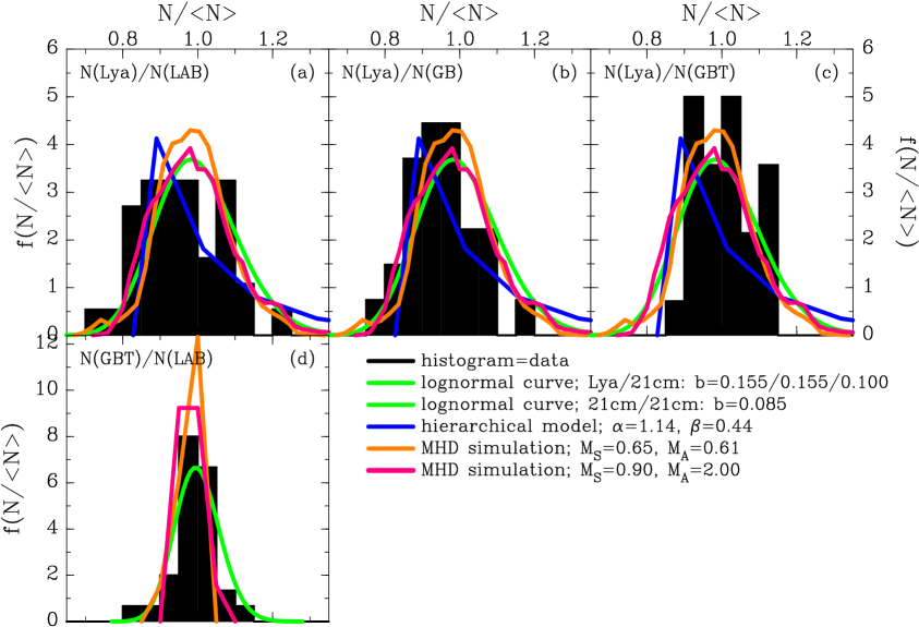
Figure 8: Plot examining the distribution of $N$/$\bar{N}$ ratio measurements. The horizontal axis is the ratio value and the vertical axis is the relative frequency of each ratio, with the curves normalized so that the integral under each curve is 1. The filled black histograms give the observed ratios for all combinations of $N$(H I) derived from Ly$\alpha$, Leiden-Argentina-Bonn survey (LAB), the Green Bank 140-ft (GB) and the Green Bank Telescope (GBT). All Ly$\alpha$ data are used, independent of quality factor; using only Q=3/4 data does not qualitatively change these histograms. For the 21-cm vs. 21-cm comparisons only the low-velocity gas components are used. The green curve is a theoretical log-normal distribution, with three different $b$ parameters (see text). The blue curve is the hierarchical model with $\alpha$=1.14 and $\beta$=0.44. The orange and red curves are the distributions obtained from taking random pencil beam measurments in two different simulations of 3D MHD turbulence, using the given sonic (M_S) and Alfvenic (M_A) Mach numbers.

5.2.2 Assuming that the distribution is log-normal

It is likely that the structure of Galactic H I is determined by turbulence (see e.g. Kowal et al. 2007; Burkhart et al. 2009). The resulting 3-D structure is then effectively determined by a multiplicative random walk. That is, a parcel of gas will be compressed and will expand proportionally to its current density. Intuitively, this should produce a column density distribution that is log-normal, i.e., the log of the density has a gaussian distribution around some mean. In most circumstances, if the 3-D turbulence produces a log-normal distribution of volume densities, the 2-D column density projection will also be log-normal.

We note that converting a log-normal distribution to a linear scale results in the mode being at a value below the average. Taking a random sampling of sightlines through the gas gives a distribution with the mode at some density. Averaging this same parcel of gas by observing it with a large beam will thus result in a value slightly larger than the mode. The offset is determined by the width of the distribution. Using $N_{m}$ for the mode of the distribution, we can write:

$$f(N/N_{m})=\exp\left(-{\left(\ln\,N/N_{m}\over b\right)^{2}}\right),$$

where $f(N/N_{m})$ is the log-normal distribution of the column densities and $b$ is a parameter characterizing the width of the distribution. The column densities are normalized to the modal value, $N_{m}$, The average value of $N$ observed in the area of integration, $\bar{N}$ is then found to be:

$${\bar{N}\over N_{m}}={\int N/N_{m}\ f(N/N_{m})dN\over\int f(N/N_{m})dN}.$$

To compare this to $N$(H I; Ly$\alpha$)/$N$(H I; 21cm), we have to invert this, since $N$(H I; Ly$\alpha$) corresponds to $N$, the column density in each pencil beam inside the area of averaging, while $N$(H I; 21cm) corresponds to $\bar{N}$. Then the integral works out to be:

$${N_{m}\over\bar{N}}=\exp{-3b^{2}\over 4}.$$

Thus, taking for instance $b$=0.155, the ratio of mode to average is 0.98, while for $b$=0.25 it is 0.95.

We have too few sightlines to determine whether the mode of the distribution of ratios differs significantly from 1. However, we can match the dispersion of the log-normal distribution to the observations. For the Ly$\alpha$/LAB, Ly$\alpha$/140-ft and Ly$\alpha$/GBT ratios this requires $b$=0.155, 0.126 and 0.101, respectively. For GBT/LAB, 140-ft/LAB and GBT/140-ft the required $b$=0.085, 0.094 and 0.043. The green curves in Fig. 8 show two log-normal distributions. For the Ly$\alpha$ to LAB and 140-ft comparisons we used $b$=0.155, while for comparing Ly$\alpha$/GBT we used $b$=0.100, the values for which the dispersions match. In the case of comparing 21-cm to 21-cm data, we used $b$=0.085, which matches the GBT/LAB dispersion. Clearly, a log-normal distribution resembles the observed distributions. It is unclear whether it is significant that the distribution of Ly$\alpha$/LAB ratios is wider than that of Ly$\alpha$/GBT ratios, but it might in principle be possible to attribute this to the fact that the GBT beam samples a smaller region, so that the relative fluctuations are smaller.

5.2.3 Using the results of a 3D MHD simulation

Kowal et al. (2007) presented a set of simulations of turbulence. We used the model datacubes that they produced to extract column densities by projecting these cubes onto one of their faces. We added to this some cubes made with the same software, but which were not included in their paper. These cubes can be projected onto one axis and converted to a table of 65536 column densities. We then plotted the distribution of these column densities, normalizing by the average of all column densities ($\bar{N}$) in the simulation. Kowal et al. (2007) used the gas and magnetic Mach numbers to parametrize their simulations. In fact, there is a distribution of Mach numbers throughout their cubes, and the numbers represent the average Mach numbers.

We extracted the predicted column density distributions for each of 16 simulations, and compared them to the data. In Fig. 8 the orange and red curves give the theoretical distributions of ratios, $N$/$\bar{N}$, for the two best models, which are the cases with sonic and Alfvenic Mach numbers of ($M_{S}$,$M_{A}$)=(0.65,0.61) and ($M_{S}$,$M_{A}$)=(0.90,2.00), respectively. For models with $M_{S}$ below 0.5 the width of the distribution is much narrower than observed, while if $M_{S}$ is larger than 1.4 the predicted distribution is much wider than observed (and the mode lies near a ratio of 0.7 when $M_{S}$$>$2). In all models, the influence of the Alfvenic Mach number is modest, changing only the details of the distribution but not the width, although the models with higher $M_{A}$ fit better than those with lower $M_{A}$. It is also clear that these instances of the MHD models predict distributions that are quite similar to a log-normal distribution with $b$$\sim$0.155.

The simulations were also used to compare the GBT vs. LAB telescope pairs. In this cases, $N$ is the column density in an area that is $(10/36)^{2}$$\sim$(1/13)th times the full size of the simulation. Since none of the 21-cm telescopes actually make a pencil beam measurement, it is incorrect to use each pencil beam measurement as $N$ in these instances. When comparing, e.g., Green Bank 140-ft to LAB data, the number of 140-ft beams inside the LAB beam is only $(36/21)^{2}$$\sim$3. This means that in such cases, there is no clear difference between $N$ and $\bar{N}$, making $N$/$\bar{N}$ a trivial comparison between 21-cm telescopes of similar beam size. Thus, we only compare the GBT to the LAB data (Fig. 8d). Using our approach the predicted width of the distribution is clearly narrower than was the case for the comparison between Ly$\alpha$ and 21-cm, as is predicted by the simulations.

Our approach of comparing column densities between observations made with very different resolutions suggests a simple way of characterizing the small-scale structure of the ISM. The predictions from different 3-D turbulent MHD models are clearly sensitive to the sonic Mach number that is used. The observed distribution of ratios fits very well with those predictions. The COS instrument on HST is expected to provide the possibility of measuring $N$(H I; Ly$\alpha$) toward several 100 additional sightlines, strongly improving the statistics and thus the constraints on the model parameters. Another possibility is to use high-resolution H I data, such as those that will become available when the GALFA (see Peek & Heiles 2008) or GASKAP surveys are complete (GASKAP is a survey of the Galactic Plane to be executed with the ASKAP telescope, building of which is in progress). These surveys have 3′ and 1′ resolution, and thus provide a large dynamic range in resolution.

6 Conclusions

We derive the column density of neutral H I from the Ly$\alpha$ line using data from the STIS-spectrograph on HST, and from the 21-cm line using the Leiden-Argentina-Bonn (LAB) survey, Green Bank 140-ft and Green Bank Telescope (GBT) observations. Using these column densities, we compare the ratio of $N$(H I; Ly$\alpha$) to $N$(H I; 21cm) and $N$(H I; 21cm) to $N$(H I; 21cm) in order to analyze the structure of the ISM. Based on the results, we conclude the following:

(1) For 59 AGNs surveyed, 36 yield reliable Ly$\alpha$ column densities. There are 163 Green Bank 140-ft and 35 GBT sightlines for which $N$(H I; 21cm) is derived. For each of the unique sightlines, we also measured $N$(H I) using LAB data.

(2) We conclude that the published LAB data, as well as our old (from the late 1980s) Green Bank 140-ft data, suffer from a problem that results in an excess column density. of $\sim$1.5$\times 10^{19}$ ${\rm cm^{-2}}$. This problem is revealed by extracting the spectral regions outside the range where signal appears to be present. There is no residual emission in the combined GBT spectrum, in contrast to the LAB and 140-ft data. The residual can be fitted by a gaussian, which for the LAB dataset has $v$=$-$22 km s^-1, $T$=0.048 K and FWHM=167 km s^-1. The parameters of the residual are different for the 1 km s^-1 and 2 km s^-1 channel spacing 140-ft spectra.

(3) We conclude that the H I spectra from the LAB survey need to be corrected for the presence of a broad underlying gaussian. Without such a correction, the LAB data conflict with measurements of $N$(H I) made with the GBT and made using Ly$\alpha$ absorption, as well as with UV absorption-line studies, and with the properties of the recently-found population of small H I clouds. With such a correction, all tension between measures of $N$(H I) at different resolutions disappears.

(4) Using data from the FOS on HST, Savage et al. (2000) had found that on average $N$(H I; Ly$\alpha$)/$N$(H I; 21cm) was 0.81$\pm$0.09 for 12 sightlines. Using our new data, the same set of sightlines yields Ly$\alpha$ column densities that are on average $\sim$0.06 dex higher (compared to the typical error of 0.2–0.3 dex in the FOS results). We also find that a correction is needed to the 140-ft data, which corresponds to 0.05 dex in these 12 sightlines. As a result of these corrections, the average ratio $N$(H I; Ly$\alpha$)/$N$(H I; 21cm) for these sightlines is now found as 1.02$\pm$0.08.

(5) After applying the corrections to the LAB and 140-ft observations, we find that the ratios between $N$(H I; Ly$\alpha$) and $N$(H I; 21cm) are on average 0.96$\pm$0.11 (Ly$\alpha$/LAB), 0.95$\pm$0.09 (Ly$\alpha$/140-ft) and 1.00$\pm$0.07 (Ly$\alpha$/GBT). A statistical test shows that these averages do not differ from 1 in a statistically significant way.

(6) A hierarchical model for the ISM matches the observed column density distribution for $N$(H I; Ly$\alpha$)/$N$(H I; 21cm) ratios adequately well, although it underpredicts the number of high ratios.

(7) A log-normal model matches column density ratio distribution moderately well, with a different width parameter for different cases.

(8) Using a 3-D MHD model from Kowal et al. (2007), we can match most features of the column density distributions when choosing cases with $M_{S}$=0.65–0.90. These distributions are similar to a simple log-normal distribution, as is expected for turbulence.

(9) We conclude that by comparing H I column densities observed at very different resolutions it becomes possible to characterize the small-scale structure of the ISM. Although the number of sightlines in our sample is small, the distribution of column density ratios approximately follows a log-normal distribution, which is also similar to the predictions of 3-D MHD modeling, using a sonic Mach number in the range 0.65-0.90.

Acknowledgements

BPW acknowledges support from NSF grant AST-0607154 and NASA-ADP grant NNX07AH42G. The Green Bank Telescope is part of the National Radio Astronomy Observatory, a facility of the NSF operated under cooperative agreement by Associated Universities, Inc. The Ly$\alpha$ data in this paper were obtained with the NASA ESA Hubble Space Telescope, at the Space Telescope Science Institute, which is operated by the Association of Universities for Research in Astronomy, Inc. under NASA contract NAS5-26555. Spectra were retieved from the Multimission Archive (MAST) at STScI. We thank UW graduate students Alex Hill and Blakesley Burkhart for extracting the column densities from the simulation of Kowal et al. (2007) and for providing additional models. JMB acknowledges Steve Schmitt and Erin Conrad for mathematical discussions. We thank the anonymous referee for insisting that we investigate possible errors in the 21-cm surveys.

Appendix

3C 249.1 – The quality factor of the column density determination is only 2, because the spectrum is relatively noisy and the 21-cm spectrum shows the presence of several IVCs. There is an unidentified line near 1210 Å, which cannot be intergalactic Ly$\alpha$, but which also does not fit into any known system of absorbers toward this sightline.

3C 273.0 – Intrinsic O VI emission at 1195.32 Å and 1201.91 Å creates a moderately broad peak in the continuum at wavelengths shorter than Galactic Ly$\alpha$. Combined with the intermediate-velocity gas at $v$$\sim$25 km s^-1  this leads us to assign quality 2 to this sightline. A third order polynomial fits the right side of the O VI wing well and creates a good fit overall from 1197 Å to 1247 Å.

3C 351.0 – The spectrum of this AGN is flat near Galactic Ly$\alpha$, and the 21-cm spectrum is simple, resulting in quality factor 4 for this spectrum.

H 1821+643 – The continuum of this target is flat and does not contain features. However, there are weak H I components at high negative velocities ($<$$-$100 km s^-1), lowering the confidence in the resulting value of $N$(H I) and leading us to give quality 3 to this target.

HE 0226$-$4110 – The spectrum of this AGN is flat near Galactic Ly$\alpha$, and the 21-cm spectrum is simple, resulting in quality factor 4 for this spectrum. Where we find a value of 20.09$\pm$0.04 for the H I columm density, Savage et al. (2007) reported 20.12$\pm$0.03 based on an earlier analysis of the same data.

HE 0340$-$2703 – Uncertain continuum placement due to the presence of multiple strong IGM lines results in a low quality fit for this QSO continuum. In addition, on the short-wavelength side there appears to be an (unidentified) intrinsic emission line, making the continuum even more uncertain. We therefore assign Q=1 to this target.

HE 1029$-$1401 – The spectrum of this AGN is flat near Galactic Ly$\alpha$, and the 21-cm spectrum is simple, resulting in quality factor 4 for this spectrum.

HE 1228+0131 – The noisy continuum of this spectrum makes it is impossible to obtain a good fit. This is further complicated by the lack of knowledge about the intrinsic continuum of the QSO, which is higher at $\lambda$$<$1215 Å than at $\lambda$$>$1215 Å. Intrinsic S IV $\lambda$1062.664 (redshifted to 1186 Å) and intrinsic N II $\lambda$1083.994 (redshifted to 1211 Å) emission may be present, and there is also a steep continuum drop across Galactic Ly$\alpha$. These problems make the continuum too uncertain to fit, and we do not use this sightline in our analysis.

HS 0624+6907 – The spectrum of this AGN is flat near Galactic Ly$\alpha$, but the 21-cm spectrum is not simple, resulting in quality factor 2 for this spectrum.

HS 1543+5921 – A complicated continuum combined with low S/N make a good fit for the continuum almost impossible. In particular, Ly$\alpha$ absorption in SBS 1543+593 at 2800 km s^-1 blends with Galactic Ly$\alpha$. We do not use this spectrum in our analysis.

HS 1700+6416 – The continuum is too difficult to obtain a good fit due to multiple IGM lines and moderate to high noise. We do not use this spectrum in our analysis.

MCG +10-16-111 – The 21-cm spectrum shows two components of similar strength. As explained in Sect. 2.2, we fix each one in turn and fit the other, in order to determine a systematic error. As can be seen in Table 2, the sum of the two stays more or less constant. As we cannot reliably compare the 21-cm and Ly$\alpha$ column densities, we assign Q=1 to this sightline.

MRC 2251$-$178 – Intrinsic Ly$\alpha$ emission peaks at 1296 Å, creating a moderately strong emission wing for measuring the Galactic Ly$\alpha$ absorption. A third order polynomial provides a good fit from 1195 Å to 1241 Å. Since the 21-cm spectrum is simple and the upward slope is minor, we assign Q=3 to this sightline.

Mrk 110 – Intrinsic Ly$\alpha$ emission peaks at 1259 Å, creating an upward slope in the continuum. A third order polynomial fits this wing adequately and provides an adequate fit for the rest of the continuum in the wavelength range plotted, resulting in Q=3.

Mrk 205 – The 21-cm spectrum contains multiple H I components including absorption originating in NGC 4319 at 1289 km s^-1 and an HVC at $v$=$-$204 km s^-1. The HVC is relatively strong, resulting in a 0.04 dex systematic error in the value of $N$(H I; Ly$\alpha$) for the Galactic emission. Extra curvature is present in the continuum and a second order polynomial was used to handle this. On balance, however, the result is reliable and we assign Q=3.

Mrk 279 – Many factors contribute to a low quality (Q=1) fit. Multiple H I components are present in the 21-cm spectrum, but only one component at $v$=$-$40 km s^-1 is used for the fitting. Strong Ly$\alpha$ emission is also present at 1252.69 Å creating a large wing in the continuum. A fourth order polynomial is used to handle these features and fits the continuum adequately well.

Mrk 335 – Intrinsic Ly$\alpha$ emission peaks at 1247.02 Å, creating a large wing beginning around 1208 Å and producing significant curvature in the continuum. A fourth order polynomial fits this continuum moderately well.

Mrk 478 – An order three polynomial is needed to handle the curvature in the continuum, but the fitting lines provide a good fit over the range of 1201 Å to 1234 Å. The curvature is caused by intrinsic Fe III-1122 emission, centered at 1209.02 Å.

Mrk 509 – The 21-cm spectrum contains multiple components, including an IVC at $v$=61 km s^-1. All components were included in the measurement of the 21-cm and Ly$\alpha$ H I column density. Strong intrinsic Ly$\alpha$ emission at 1256 Å creates a large wing. A fourth order polynomial fits this wing and the continuum well from 1180 Å to 1230 Å.

Mrk 771 – The continuum is flat across the Galactic Ly$\alpha$ line. Although the 21-cm spectrum show two strong components, their separation in velocity is low enough that the final fit to the Ly$\alpha$ absorption results in Q=4.

Mrk 876 – The 21-cm spectrum shows multiple H I components, including an HVC at $v$=$-$130 km s^-1, thus a systematic error in the $N$(H I) value is present due to the HVC’s impact. Intrinsic O VI emission at 1165 Å and 1171 Å also causes the continuum to slope downward at the short-wavelength side of Ly$\alpha$, but an order two polynomial still provides a good fit. These complications lead us to assign quality factor 2 to this measurement.

Mrk 926 – A third order polynomial provides a good fit to the continuum. However, multiple factors contribute to a systematic error in the value of $N$(H I). One factor is strong intrinsic Ly$\alpha$ emission at 1273 Å that creates a broad wing in the continuum. Another factor is the fact that the G140M appears to show an extra upturn to the continuum below wavelengths of 1200 Å (not easily visible in Fig. 5). Combined with a relatively noisy spectrum, we decided to assign Q=1 to this sightline.

Mrk 1044 – Strong instrinsic Ly$\alpha$ emission at 1235.86 Å adds a large wing to the continuum. A fourth order polynomial fits this wing well and fits the continuum adequately from 1203 Å to 1223 Å. The strong curvature across Ly$\alpha$ results in Q=2 for this target.

Mrk 1383 – An order two polynomial is needed to handle the slight curvature in the continuum, but the fit is still good enough to derive a result with quality factor 4.

Mrk 1513 – The continuum is flat, except near 1197 Å where it shows an upturn, although there are no known intrinsic emission features near this wavelength. The tail-end of intrinsic Ly$\alpha$ emission also causes the continuum to rise at wavelengths above 1235 Å. The net result of both issues is that the continuum fit is not as reliable as it might seem, resulting in quality 3 for this measurement.

NGC 985 – Intrinsic Ly$\alpha$ emission peaks at 1268 Å, creating a moderate upward slope near Galactic Ly$\alpha$. A third order polynomial provides a good fit from 1195 Å to 1240 Å.

NGC 1705 – The continuum is too complicated to make a good fit due to intrinsic N V emission at 1241.42 Å and 1245.41 Å as well as intrinsic Ly$\alpha$ emission from the galaxy, which has a redshift of only 628 km s^-1. Therefore, we do not derive $N$(H I; Ly$\alpha$) for this sightline.

NGC 3516 – The continuum is too difficult to obtain a good fit due to moderate to high noise and strong intrinic Ly$\alpha$ emission at 1225 Å. Therefore, we do not derive $N$(H I; Ly$\alpha$) for this sightline.

NGC 3783 – The continuum is too difficult to obtain a good fit due to the strong Ly$\alpha$ emission at 1227.50 Å, as well as the presence of multiple strong H I components at intermediate and high velocity. Therefore, we do not derive $N$(H I;Ly$\alpha$) for this sightline.

NGC 4051 – Strong Ly$\alpha$ emission at 1218.51 Å and N V emission at 1241.71 Å and 1245.71 Å creates a continuum too difficult to obtain a good fit.

NGC 4151 – The continuum is too difficult to make a good fit due to strong Ly$\alpha$ emission at 1219.70 Å and N V emission at 1242.93 Å and 1246.93 Å.

NGC 5548 – Strong Ly$\alpha$ emission at 1236.55 Å adds a large wing to the continuum. A fourth order polynomial provides an adequate fit. Since the 21-cm profile is simple, the measurement is given a final quality of 3.

NGC 7469 – Ly$\alpha$ emission at 1235.51 Å creates a large rise in the continuum, but this is fit adequately well by a fourth order polynomial over the range of 1197 Å to 1230 Å. This results in a quality 3 measurement.

PG 0804+761 – The continuum is flat from 1201 Å to 1234 Å but is pushed above the fitting line at 1196 Å and below at 1245 Å. The final fit is given quality 3.

PG 0953+414 – Intrinsic C III emission is present at 1204.92 Å  which adds curvature that creates a hill in the continuum over a range from 1188 Å to 1236 Å. A fourth order polynomial fits this hill well over a range of 1205 Å to 1248 Å, but the curvature leads us to assign Q=3 to this measurement.

PG 1001+291 – The quality of this continuum is diminished by multiple factors, including a moderate S/N ratio and the continuum resting above the fitting line at 1183 Å.

PG 1004+130 – A high level of noise in the continuum makes it difficult to obtain a good quality fit and a reliable value of $N$(H I) for this QSO.

PG 1049$-$005 – The continuum is flat, but the high level of noise greatly reduces the quality of the fit. As a result, we assign Q=1 to this sightline.

PG 1103$-$006 – Low S/N makes obtaining a reliable fit impossible for this target.

PG 1116+215 – The intrinsic O VI emission lines are redshifted to 1214.06 Å and 1220.75 Å, which results in a large bump in the continuum across the Galactic Ly$\alpha$ line. This can be modeled by using a fourth order polynomial, which fits the continuum adequately well from 1180 Å to 1248 Å. The 21-cm spectrum shows two components of similar strength at $-$39 and $-$5 km s^-1. These factors combine to yield Q=1 for the resulting Ly$\alpha$ column density.

PG 1149$-$110 – Intrinsic Ly$\alpha$ emission peaks at 1275.24 Å and a low S/N ratio make a good fit for the continuum too difficult to obtain.

PG 1211+143 – Intrinsic Fe III $\lambda$1122.52 emission is redshifted to 1212.77 Å, which pushes the continuum slightly upward on the short-wavelength side of Galactic Ly$\alpha$. This lowers the quality of the fit, although a fourth order polynomial is used and fits the continuum adequately well from 1180 Å to 1248 Å. The final fit quality is assigned a value of 3.

PG 1259+593 – Multiple H I components are present in the continuum including an HVC at $v$=$-$127 km s^-1 and an IVC at $v$=$-$52 km s^-1. A two-sided fit is used, as described in Sect. 2.2.

PG 1302$-$102 – The continuum is flat, but the low S/N visibly diminishes the quality of the fit.

PG 1341+258 – The continuum is slightly above the fitting line from 1223 Å to 1230 Å, but a linear fit still provides a high quality (Q=4) fit.

PG 1351+640 - The continuum contains multiple absorption features, lowering the quality of the fit. The 21-cm spectrum shows multiple H I components including an HVC at $v$=$-$156 km s^-1. Thus, a systematic error is introduced into the value for $N$(H I) due to the HVC’s impact on the continuum. Intrinsic Fe III emission is also present at 1221.53 Å. Although a fourth order polynomial is used to deal with these features and provides an adequate fit for the continuum, the uncertainty associated with the HVC’s column density is such that we assign a final quality factor of 1.

PG 1444+407 – A flat continuum gives an acceptable fit. However, it is a little above the fitting line from 1180 Å to 1200 Å and from 1233 Å to 1237 Å, thus reducing the quality of this fit. Combined with the multiple 21-cm components, the final column density value is quality 2.

PHL 1811 – A flat continuum is a good fit despite the presence of intrinsic O VI emission at 1230.06 Å and 1236.84 Å, which pushes the continuum slightly above the fitting line from 1224 Å to 1236 Å. Combined with the simplicity of the 21-cm profile, the final quality for this sightline is 4.

PKS 0312$-$77 – The 21-cm spectrum contains multiple H I components, including the Magellanic Bridge at $v$=191 km s^-1 and $v$=166 km s^-1. A two-sided fit is used as described in Sect. 2.2. Lehner et al. (2008) gives Ly$\alpha$-derived column densities of 20.78$\pm$0.06 and 20.12$\pm$0.30 for components at 5 and 210 km s^-1, respectively. The combined value is 20.86. From the LAB data, we find a column densities of 20.83 and 20.23 for these two components. Varying the Magellanic Bridge component between 20.14 and 20.31 results in values for the low-velocity column density of 20.67$\pm$0.18 to 20.71$\pm$0.17. A combined fit yield values between 20.79$\pm$0.14 and 20.87$\pm$0.11, depending on the precise selections. Thus, we find a column density for the Magellanic Bridge component that is 0.1 dex higher than that of Lehner et al, but within their error. We also find that Lehner et al. underestimated the error for the low-velocity gas by a factor $\sim$3.

PKS 0405$-$12 – The continuum is flat but a few extra features reduce the quality of the fit. There may be Ne VIII emission at 1211.06 Å and intrinsic O IV emission at 1238.75 Å. N III emission at 1200.42 Å pushes the continuum up slightly, and a dip from 1243 Å to 1255 Å pulls the continuum down, creating a twist in the continuum that causes the fitting line to slope upward. In the end, we only assign Q=2 to this sightline.

PKS 2005$-$489 – This spectrum is flat across Galactic Ly$\alpha$, and the sightline has a simple 21-cm profile. The derived Ly$\alpha$ column density is quality four.

PKS 2155$-$304 – This spectrum is flat across Galactic Ly$\alpha$, and the sightline has a simple 21-cm profile. The derived Ly$\alpha$ column density is quality four.

RX J0100.4$-$5113 – The continuum placement is too uncertain for this QSO to obtain a good fit or a reliable value for $N$(H I). The continuum is further complicated by the presence of an HVC at $v$=92 km s^-1.

RX J1830.3+7312 – The moderate curvature of the continuum reduces the quality of the fit to Q=3, but a third order polynomial still provides a good fit for this QSO.

Ton S180 – The fit is of lower quality due to significant curvature in the continuum. This results from the intrinsic Ly$\alpha$ line centered at 1291 Å, and a rise toward the lower wavelength edge that is seen in many G140M spectra, which is probably due to a calibration problem.

Ton S210 – The fit is of lower quality due to multiple factors. One is the moderate S/N. Another is the uncertainty of the continuum, which rises toward the lower wavelengths due to the wing of the intrinsic O VI emission, centered at about 1155 Å.

UGC 12163 – This spectrum is relatively noisy, and the wing of the intrinsic Ly$\alpha$ line, centered at 1245 Å, extends above the Galactic Ly$\alpha$ absorption, making a determination of the continuum almost impossible.

VII Zw 118 – A flat continuum is present, but the slope combined with a continuum dip between 1195 Å to 1205 Å reduces the quality of the fit.

References

- (1) Blagrave K., Lockman F.J., Martin P.G.J., 2010, arXiv 1009.0715
- (2) Burkhart B., Falceta-Gon calves D., Kowal G., Lazarian A., 2009, ApJ, 693, 250
- (3) Falgarone E., Philips T.G., Walker C.K., 1991, ApJ, 378, 186
- (4) Ford A.H., Lockman F.J., McClure-Griffiths N.M., 2010, arXiv, 1008, 2760
- (5) Ford A.H., McClure-Griffiths N.M., Lockman F.J., Bailin J., Calabretta M.R., Kalberla P.M.W., Murphy T., Pisano D.J., 2008, ApJ, 688, 290
- (6) Hartmann D., Burton W.B., 1997, “Atlas of Galactic Neutral Hydrogen”, ISBN 0521471117, Cambridge, UK: Cambridge University Press
- (7) Heiles C., Troland T.H., 2003, ApJ, 586, 1067
- (8) Hobbs L.M., Morgan W.W., Albert C.E., 1982, ApJ, 263, 690
- (9) Houlahan P., Scalo J., 1992, ApJ, 393, 172
- (10) Kalberla P.M.W., Mebold U., Reif K., 1982, A&A, 106, 190
- (11) Kalberla P.M.W., Westphalen G., Mebold U., Hartmann D., Burton W.B., 1998, A&A, 332, L61
- (12) Kalberla P.M.W., Burton W.B., Hartmann D., Arnal E.M., Bajaja E., Morras R., Pöppel W.G.L., 2005, A&A, 440, 775
- (13) Kowal G., Lazarian A., Bersnyak A., 2007, ApJ, 658, 423
- (14) Lazarian A., Pogosyan D., 2000, ApJ, 537, 72
- (15) Lazarian A., Pogosyan D., 2004, ApJ, 616, 943
- (16) Lazarian A., Pogosyan D., 2006, ApJ, 652, 1348
- (17) Lazarian A., Pogosyan D., 2008, ApJ, 686, 350
- (18) Lehner N., Howk J.C., Keenan F.P., Smoker J.V., 2008, ApJ, 678, 219
- (19) Lockman F.J., Hobbs L.M., Shull J.M., 1986a, ApJ, 301, 380
- (20) Lockman F.J., Jahoda K., McCammon D., 1986b, ApJ, 302, 432
- (21) Lockman F.J., Savage B.D., 1995, ApJS, 97, 1
- (22) Lockman F.J., 2002, ApJ, 580, 47
- (23) Lockman F.J., Benjamin R.A., Heroux A.J., Langston G.I., 2008, ApJL, 679, L21
- (24) Ott M., Witzel A., Quirrenbach A., Krichbaum T.P., Standke K.J., Schalinski C.J., Hummel C.A., 1994, A&A, 284, 331
- (25) Peek J.E.F., Heiles C., 2008, arXiv 0810.1283
- (26) Penzias A.A., Wilson R.W., Encrenaz P.J., 1970, AJ, 75, 141
- (27) Prestage R.M., Constantikes K.T., Hunter T.R., King L.J., Lacasse R.J., Lockman, F.J., Norrod D., 2009, Proc. of the IEEE, Vol. 97, p1382
- (28) Robishaw T., Heiles C., 2009, PASP, 121, 272
- (29) Savage B.D., Wakker B.P., Jannuzi B.T., Bahcall J.N., Bergeron J., et al. 2000, ApJS, 129, 563
- (30) Savage B.D., Lehner N., Fox A., Wakker B.P., Sembach K.R., 2007, ApJ, 659, 1222
- (31) Sembach, K.R., Savage, B.D., 1992, ApJS, 83, 147
- (32) Vogelaar M.G.R., Wakker B.P., 1994, A&A, 291, 557
- (33) Wakker B.P., Savage B.D., Sembach K.R., et al., 2003, ApJS, 146, 1
- (34) Williams D.R.W., 1973, A&ApS, 8, 505
- (35) Wrixon G.T., Heiles C., 1972, A&Ap, 18, 444