Universal Polynomials for
Severi Degrees of Toric Surfaces

Abstract.

The Severi variety parameterizes plane curves of degree $d$ with $\delta$ nodes. Its degree is called the Severi degree. For large enough $d$, the Severi degrees coincide with the Gromov-Witten invariants of ${\mathbb{C}}{\mathbb{P}}^{2}$. Fomin and Mikhalkin (2009) proved the 1995 conjecture that for fixed $\delta$, Severi degrees are eventually polynomial in $d$.

In this paper, we study the Severi varieties corresponding to a large family of toric surfaces. We prove the analogous result that the Severi degrees are eventually polynomial as a function of the multidegree. More surprisingly, we show that the Severi degrees are also eventually polynomial “as a function of the surface”. We illustrate our theorems by explicit computing, for a small number of nodes, the Severi degree of any large enough Hirzebruch surface and of a singular surface.

Our strategy is to use tropical geometry to express Severi degrees in terms of Brugallé and Mikhalkin’s floor diagrams, and study those combinatorial objects in detail. An important ingredient in the proof is the polynomiality of the discrete volume of a variable facet-unimodular polytope.

1. Introduction and Main Theorems

1.1. Severi degrees and node polynomials for ${\mathbb{C}}{\mathbb{P}}^{2}$.

A $\delta$-nodal curve is a reduced (not necessarily irreducible) curve having $\delta$ simple nodes and no other singularities. The Severi degree $N^{d,\delta}$ is the degree of the Severi variety parameterizing degree $d$ $\delta$-nodal curves in the complex projective plane ${\mathbb{C}}{\mathbb{P}}^{2}$. In other words, $N^{d,\delta}$ is the number of such curves through an appropriate number of points in general position. For $d\geq\delta+2$, $N^{d,\delta}$ equals the Gromov-Witten invariant $N_{d,{d-1\choose 2}-\delta}$.

Severi varieties were introduced around 1915 by Enriques [8] and Severi [20], and have received considerable attention. Much later, in 1986, Harris [13] achieved a celebrated breakthrough by proving their irreducibility.

In 2009, Fomin and Mikhalkin [9, Theorem 5.1] proved Di Francesco and Itzykson’s 1995 conjecture [7] that, for a fixed number of nodes $\delta$, the Severi degree $N^{d,\delta}$ becomes a polynomial $N_{\delta}(d)$ in the degree, for $d\geq 2\delta$. We will call $N_{\delta}(d)$ the node polynomial following Kleiman–Piene [14]. In [3], the second author improved the threshold of Fomin and Mikhalkin from $2\delta$ to $\delta$ and computed the node polynomials for $\delta\leq 14$ extending work of Kleiman and Piene [14] for $\delta\leq 8$.

1.2. Severi degrees and node polynomials for toric surfaces.

The purpose of this paper is to generalize the previous results to the context of counting curves on a large family of (possibly non-smooth) toric surfaces ${\mathrm{S}}({\bf c})$, which includes ${\mathbb{C}}{\mathbb{P}}^{1}\times{\mathbb{C}}{\mathbb{P}}^{1}$ and Hirzebruch surfaces. A new and interesting feature of our results is that the Severi degree $N^{{\bf d},\delta}_{{\mathrm{S}}({\bf c})}$ of such a toric surface ${\mathrm{S}}({\bf c})$ is a polynomial not only as a function of the degree ${\bf d}$, but also as a function of ${\bf c}$, i.e., as a “function of the surface” itself.

A note for combinatorialists. A familiarity with the basic facts of toric geometry is desirable to understand the motivation for this work (and we refer the reader to Fulton’s book [11] for the necessary definitions and background information). However, the machinery of tropical geometry allows for a purely combinatorial approach to studying Severi degrees, and most of this paper can be read independently of that background.

We now state our results more precisely.

Notation 1.1.

A polygon $P$ is said to be $h$-transverse if it has integer coordinates and every edge has slope $0$, $\infty$, or $\frac{1}{k}$ for some integer $k$. Let $d^{\,t}$ and $d^{\,b}$ be the lengths of the top and bottom edges of $P$, if they exist (and 0 if they don’t exist). Let the edges on the right side of the polygon, listed clockwise from top to bottom, have directions $(c^{r}_{1},-1),\ldots,(c^{r}_{n},-1)$ and lattice lengths $d^{\,r}_{1},\ldots,d^{\,r}_{n}$, so $c^{r}_{1}>\cdots>c^{r}_{n}$. Let the edges on the left side of the polygon, listed counterclockwise from top to bottom, have directions $(c^{l}_{1},-1),\ldots,(c^{l}_{m},-1)$ and lattice lengths $d^{\,l}_{1},\ldots,d^{\,l}_{m}$, so $c^{l}_{1}<\cdots<c^{l}_{m}$. Notice that $d^{\,t}+\sum_{i}c^{r}_{i}d^{\,r}_{i}-d^{\,b}-\sum_{j}c^{l}_{j}d^{\,l}_{j}=0$.

Denote ${\bf c}^{r}=(c^{r}_{1},\ldots,c^{r}_{n})$, ${\bf d}^{r}=(d^{\,r}_{1},\ldots,d^{\,r}_{n})$, ${\bf c}^{l}=(c^{l}_{1},\ldots,c^{l}_{m})$, ${\bf d}^{l}=(d^{\,l}_{1},\ldots,d^{\,l}_{m})$, and ${\bf c}=({\bf c}^{r};{\bf c}^{l}),{\bf d}=(d^{\,t};{\bf d}^{r};{\bf d}^{l})$. Finally, denote $\Delta({\bf c},{\bf d}):=P$. Observe that ${\bf c}$ is the set of slopes of the non-vertical rays in the normal fan of $\Delta({\bf c},{\bf d})$.

Figure 1 shows the polygon $\Delta({\bf c},{\bf d})$ with ${\bf c}=((3,1,0,-1);(-2,0,1,2))$ and    ${\bf d}=(1;(1,2,1,1);(1,1,1,2))$ and its normal fan.

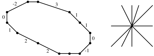
Figure 1. An $h$-transverse polygon and its normal fan.

The normal fan of the polygon $\Delta({\bf c},{\bf d})$ consists of the outward rays centered at the origin and perpendicular to the sides. This fan determines a projective toric surface ${\mathrm{S}}({\bf c})$ (which only depends on ${\bf c}$ and whether $d^{\,t}$ and $d^{\,b}$ are zero). Additionally, the polygon itself determines an ample line bundle ${\mathcal{L}}_{\bf c}({\bf d})$ on ${\mathrm{S}}({\bf c})$; let $|{\mathcal{L}}_{\bf c}({\bf d})|$ be the complete linear system of divisors on ${\mathrm{S}}({\bf c})$ corresponding to ${\mathcal{L}}_{\bf c}({\bf d})$.

When we count curves on ${\mathrm{S}}({\bf c})$, we will loosely think of ${\bf c}$ as the surface where our curves live, and ${\bf d}$ as their multidegree. This is motivated by the case when $\Delta({\bf c},{\bf d})=\textrm{conv}\{(0,0),(m,0),(0,m)\}$. In this case the toric surface is ${\mathbb{C}}{\mathbb{P}}^{2}$, and the linear system $|{\mathcal{L}}_{\bf c}({\bf d})|$ parameterizes the degree $m$ curves on ${\mathbb{C}}{\mathbb{P}}^{2}$.

Given a positive integer $\delta$, the Severi variety is the closure of the set of $\delta$-nodal curves in $|{\mathcal{L}}_{{\bf c}}({\bf d})|$. Its degree is the Severi degree $N_{{\mathrm{S}}({\bf c})}^{{\bf d},\delta}$. This number also counts:

• the $\delta$-nodal curves in $|{\mathcal{L}}_{\bf c}({\bf d})|$ which pass through a given set of $|\Delta\cap{\mathbb{Z}}^{2}|-1-\delta$ generic points in ${\mathrm{S}}({\bf c})$, and

• the $\delta$-nodal curves in the torus $({\mathbb{C}}^{*})^{2}$ defined by polynomials with Newton polygon $\Delta({\bf c},{\bf d})$ which go through a given set of $|\Delta\cap{\mathbb{Z}}^{2}|-1-\delta$ generic points in $({\mathbb{C}}^{*})^{2}$.

Our main result is that, for a fixed number of nodes $\delta$, the Severi degree $N_{{\mathrm{S}}({\bf c})}^{{\bf d},\delta}$ is a polynomial in both ${\bf c}$ and ${\bf d}$, provided ${\bf c}$ and ${\bf d}$ are sufficiently large and “spread out”, in the precise sense defined below.

Theorem 1.2.

(Polynomiality of Severi degrees 1: Fixed Toric Surface.)
Fix $m,n\geq 1$, $\delta\geq 1$, and ${\bf c}\in{\mathbb{Z}}^{m+n}$. There is a combinatorially defined polynomial $p^{\bf c}_{\delta}({\bf d})$ such that the Severi degree $N_{{\mathrm{S}}({\bf c})}^{{\bf d},\delta}$ is given by

(1.1) $$N_{{\mathrm{S}}({\bf c})}^{{\bf d},\delta}=p^{\bf c}_{\delta}({\bf d})$$

for any sufficiently large and spread out ${\bf d}\in{\mathbb{Z}}_{\geq 0}^{m+n+1}$.

More precisely, the result holds if we assume, in Notation 1.1, that:

$$d^{\,t},d^{\,b} \geq \delta,$$

$$d^{\,t}+c^{r}_{1}-c^{l}_{1},\,\,d^{\,b}+c^{r}_{n}-c^{l}_{m} \geq 2\delta,$$

$$d^{\,r}_{i},\,\,d^{\,l}_{j} \geq \delta+1\quad(1\leq i\leq n,\,\,1\leq j\leq m),$$

$$\left|(d^{\,r}_{1}+\cdots+d^{\,r}_{i})-(d^{\,l}_{1}+\cdots+d^{\,l}_{j})\right| \geq \delta+2\quad(1\leq i\leq n-1,\,\,1\leq j\leq m-1).$$

Theorem 1.3.

(Polynomiality of Severi degrees 2: Universality.)
Fix $m,n\geq 1$ and $\delta\geq 1$. There is a universal and combinatorially defined polynomial $p_{\delta}({\bf c},{\bf d})$ such that the Severi degree $N_{{\mathrm{S}}({\bf c})}^{{\bf d},\delta}$ is given by

(1.2) $$N_{{\mathrm{S}}({\bf c})}^{{\bf d},\delta}=p_{\delta}({\bf c},{\bf d})$$

for any sufficiently large and spread out ${\bf c}\in{\mathbb{Z}}^{m+n}$ and ${\bf d}\in{\mathbb{Z}}_{\geq 0}^{m+n+1}$.

More precisely, the result holds if we assume, in Notation 1.1, that:

$$d^{\,t},d^{\,b} \geq \delta,$$

$$d^{\,t}+c^{r}_{1}-c^{l}_{1},\,\,d^{\,b}+c^{r}_{n}-c^{l}_{m} \geq 2\delta,$$

$$d^{\,r}_{i},\,\,d^{\,l}_{j} \geq \delta+1\quad(1\leq i\leq n,\,\,1\leq j\leq m),$$

$$\left|(d^{\,r}_{1}+\cdots+d^{\,r}_{i})-(d^{\,l}_{1}+\cdots+d^{\,l}_{j})\right| \geq \delta+2\quad(1\leq i\leq n-1,\,\,1\leq j\leq m-1),$$

$$c^{r}_{i}-c^{r}_{i+1},\,\,c^{l}_{j+1}-c^{l}_{j} \geq \delta+1\quad(1\leq i\leq n-1,\,\,1\leq j\leq m-1).$$

Naturally, we have $p^{\bf c}_{\delta}({\bf d})=p_{\delta}({\bf c},{\bf d})$ as polynomials in ${\bf d}$ for all sufficiently spread out ${\bf c}$ (in the sense of the last condition of Theorem 1.3).

As special cases, we obtain polynomiality results for curve counts on ${\mathbb{C}}{\mathbb{P}}^{1}\times{\mathbb{C}}{\mathbb{P}}^{1}$, and Hirzebruch surfaces. In Remark 6.2 we compute the node polynomials $p_{\delta}$ for $\delta\leq 5$ for Hirzebruch surfaces. Similar results hold for toric surfaces arising from polygons with one or no horizontal edges, such as ${\mathbb{C}}{\mathbb{P}}^{2}$; see Remark 5.2.

The restriction in Theorems 1.2 and 1.3 to toric surfaces of $h$-transverse polygons is a technical assumption necessary for our proof. Floor diagrams, our main combinatorial tools, are (as of now) only defined in this situation. We expect, however, that similar results hold for arbitrary toric surfaces.

1.3. The relationship with Göttsche’s Conjecture.

Our work is closely related to Göttsche’s Conjecture [12, Conjecture. 2.1], but the precise relationship still requires clarification. Göttsche conjectured the existence of universal polynomials $T_{\delta}(w,x,y,z)$ that compute the Severi degree for any smooth projective algebraic surface $S$ and any sufficiently ample line bundle ${\mathcal{L}}$ on $S$. According to the conjecture, the number of $\delta$-nodal curves in the linear system $|{\mathcal{L}}|$ through an appropriate number of points is given by evaluating $T_{\delta}$ at the four topological numbers ${\mathcal{L}}^{2},{\mathcal{L}}K_{S},K_{S}^{2}$ and $C_{2}(S)$. Here $K_{S}$ denotes the canonical bundle, $C_{1}$ and $C_{2}$ represent Chern classes, and $LM$ denotes the degree of $C_{1}(L)\cdot C_{1}(M)$ for line bundles $L$ and $M$. Recently, Tzeng [21] proved Göttsche’s Conjecture.

If the toric surface ${\mathrm{S}}({\bf c})$ is smooth, then all four topological numbers mentioned above are polynomials in ${\bf c}$ and ${\bf d}$. In that case, Tzeng’s proof of Göttsche’s conjecture implies that, for fixed $\delta$, the Severi degrees $N_{{\mathrm{S}}({\bf c})}^{{\bf d},\delta}$ are given by a universal polynomial in ${\bf c}$ and ${\bf d}$, provided that ${\mathcal{L}}_{\bf c}({\bf d})$ is $(5\delta-1)$-ample.

Göttsche’s conjecture does not imply our results because the toric surfaces considered in Theorems 1.2 and 1.3 are almost never smooth. The surface ${\mathrm{S}}({\bf c})$ is smooth precisely when any two adjacent rays in the normal fan span the lattice ${\mathbb{Z}}^{2}$. This happens if and only if $c_{1}^{r}-c_{2}^{r}=\cdots=c_{n-1}^{r}-c_{n}^{r}=1$ and $c_{1}^{l}-c_{2}^{l}=\cdots=c_{m-1}^{l}-c_{m}^{l}=-1$.

It is natural to ask for a generalization of the four topological numbers to some class of singular surfaces, so that Göttsche’s universal polynomial $T_{\delta}(w,x,y,z)$ specializes to the polynomial of Theorem 1.3. We do not know how to do this, even for ${\mathrm{S}}({\bf c})$ with ${\bf c}=((c_{1}^{r},c_{2}^{r});(0,0))$. In general, $C_{1}(K_{S})$ is defined for any projective variety [10, Section 3]. To define $C_{2}(S)$ for singular $S$, one could pass to MacPherson’s Chern class [16], which is defined for any algebraic variety. Alternatively, for toric surfaces, $C_{2}(S)$ could also be defined via the combinatorial formula for the Chern polynomial of a toric variety. However, we checked that $T_{\delta}(w,x,y,z)$, evaluated at any of the proposed sets of numbers, gives a different polynomial and that further (topological) correction terms appear to be necessary (c.f. Section 6.2). Alternatively, evaluating $T_{\delta}(w,x,y,z)$ at the topological numbers of a smooth resolution of ${\mathrm{S}}({\bf c})$ does not yield the desired result either.

Still, the Severi degrees are uniformly given by a polynomial in ${\bf c}$ and ${\bf d}$, provided ${\bf d}$ is sufficiently large. This suggests that it may be possible to generalize Göttsche’s conjecture to a class of singular algebraic surfaces. We present some numerical data in Section 6.2.

1.4. Outline

This paper is organized as follows. In Section 2 we describe Brugallé and Mikhalkin’s tropical method for counting irreducible curves on “$h$-transverse” toric surfaces in terms of floor diagrams, and generalize it to compute Severi degrees of such surfaces. We then focus on the combinatorial enumeration of floor diagrams. In Section 3 we generalize Fomin and Mikhalkin’s “template decomposition” of a floor diagram, and express Severi degrees in terms of templates. The resulting formula is intricate and not obviously polynomial. In Sections 4 and 5 we analyze this formula in detail. After several simplifying steps, we express Severi degrees as a finite sum, where each summand is a “discrete integral” of a polynomial function over a variable polytopal domain. This allows us to prove their eventual polynomiality. In Section 4 we carry this out for “first-quadrant” $h$-transverse toric surfaces, and in Section 5 we do it for general $h$-transverse toric surfaces. The formulas we obtain for Severi degrees are somewhat complicated, but they are completely combinatorial and effectively computable. We illustrate this in Section 6 by computing the Severi degree of any large enough Hirzebruch surface for $\delta\leq 5$ nodes as well as for a family of singular toric surfaces and $\delta\leq 2$.

Acknowledgements. We thank the referee for valuable comments that helped improve this article. We also thank Benoît Bertrand and Erwan Brugallé for clarifying some details about floor diagrams. The second author thanks Eugene Eisenstein, José González, Ragni Piene, and Alan Stapledon for explaining some facts about toric surfaces and Chern classes, and Bill Fulton for valuable comments on the subject. Part of this work was accomplished at the MSRI (Mathematical Sciences Research Institute) in Berkeley, CA, USA, during the Fall 2009 semester in tropical geometry. We would like to thank MSRI for their hospitality.

2. Counting curves with floor diagrams

In this section we review the floor diagrams of Brugallé and Mikhalkin [4, 5] associated to curves on toric surfaces which come from $h$-transverse polygons. We will introduce them using notation inspired by Fomin and Mikhalkin [9] who discussed floor diagrams in the planar case.

2.1. An outline of the tropical method for counting curves.

We briefly sketch Brugallé and Mikhalkin’s technique for counting curves through a generic set of points on a toric surface. [4, 5] (They carried this out for irreducible curves, and we extend it to possibly reducible curves and Severi degrees.) We wish to count the $\delta$-nodal curves in $({\mathbb{C}}^{*})^{2}$, having Newton polygon $\Delta$, which go through sufficiently many generic points. Brugallé and Mikhalkin proved that this problem can be “tropicalized”: we can “just” count the $\delta$-nodal tropical curves with Newton polygon $\Delta$ going through a generic set of points. Roughly speaking, such a tropical curve is an edge weighted polyhedral complex in the plane which is dual to a polyhedral subdivision of $\Delta$, as shown in Figure 2.

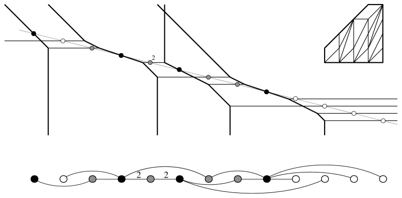
Figure 2. A tropical curve through a vertically stretched collection of 13 points (rotated $90^{\circ}$ counterclockwise), the dual subdivision of the Newton polygon (also rotated $90^{\circ}$ counterclockwise), and the corresponding marked floor diagram.

The resulting tropical enumeration problem is still very subtle. When the polygon $\Delta$ is $h$-transverse, it can be simplified. One can assume that the generic points $P$ lie very far from each other on an almost vertical line, i.e., are “vertically stretched”. In this case, one can control where the points of $P$ must land on the tropical line $L$. Divide the curve into elevators, which are all the vertical segments of $L$ (they are horizontal in Figure 2) and floors, which are the connected components of $L$ upon removal of the elevators (they are bold in Figure 2). The $h$-transversality condition then guarantees that one must have exactly one point of $P$ on each elevator and exactly one on each floor.

That geometric incidence information is then recorded in a floor diagram. This diagram has a node for each floor of $L$, and an edge for each elevator connecting two floors. More detailed information is contained in the marked floor diagram. This diagram has one black node for each floor of $L$, and one gray/white node for each bounded/unbounded elevator. Its edges show how the elevators connect the different floors of $L$.

This correspondence encodes all the necessary geometric information into combinatorial data, and reduces the computation to a (still very subtle) purely enumerative problem on marked floor diagrams. We now define marked floor diagrams precisely, and explain how exactly we need to count them.

2.2. Counting irreducible curves via connected floor diagrams.

Given a lattice polygon $\Delta$ and a positive integer $\delta$, let $N_{\Delta,\delta}$ be the number of $\delta$-nodal irreducible curves in the torus $({\mathbb{C}}^{*})^{2}$, given by polynomials with Newton polygon $\Delta$, which go through $|\Delta\cap{\mathbb{Z}}^{2}|-1-\delta$ generic points in $({\mathbb{C}}^{*})^{2}$. When the toric surface is Fano, these are the Gromov-Witten invariants of the surface ${\mathrm{S}}(\Delta)$. (These numbers should not be confused with the closely related $N^{\Delta,\delta}$, which counts curves that are not necessarily irreducible.)

We now explain how these numbers can be computed tropically, following Brugalle and Mikhalkin’s work. [4, 5]

For the rest of the paper we will assume that $\Delta=\Delta({\bf c},{\bf d})$ is $h$-transverse and we will use Notation 1.1 to describe it. Define the multiset $D_{r}$ of right directions of $\Delta$ to be the multiset containing each right direction $c^{r}_{i}$ repeated $d^{\,r}_{i}$ times. Define $D_{l}$ analogously. The cardinality of $D_{r}$ (or, equivalently, of $D_{l}$) is the height of $\Delta$.

Example 2.1.

For the polygon $\Delta$ of Figure 1, the multisets of left directions and right directions are $D_{l}=\{-2,0,1,2,2\}$ and $D_{r}=\{3,1,1,0,-1\}$ and the upper edge length is $d^{\,t}=1$.

Fix an $h$-transverse polygon $\Delta$. Now we define the combinatorial objects which, when weighted correctly, compute $N_{\Delta,\delta}$.

Definition 2.2.

A $\Delta$-floor diagram ${\mathcal{D}}$ consists of:

• two permutations $(l_{1},\dots l_{M})$ and $(r_{1},\dots r_{M})$ of the multisets $D_{l}$ and $D_{r}$ of left and right directions of $\Delta$, and a sequence $(s_{1},\dots s_{M})$ of non-negative integers such that $s_{1}+\cdots+s_{M}=d^{\,t}$,

• a graph on a vertex set $\{1,\dots,M\}$, possibly with multiple edges, with edges directed $i\to j$ for $i<j$, and

• edge weights $w(e)\in{\mathbb{Z}}_{>0}$ for all edges $e$ such that for every vertex $j$,

  $${\text{div}}(j):=\sum_{\tiny\begin{array}[]{c}\text{edges }e\\ j\stackrel{{\scriptstyle e}}{{\to}}k\end{array}}w(e)-\sum_{\tiny\begin{array}[]{c}\text{edges }e\\ i\stackrel{{\scriptstyle e}}{{\to}}j\end{array}}w(e)\leq r_{j}-l_{j}+s_{j}.\,$$

Sometimes we will omit $\Delta$ and call ${\mathcal{D}}$ a toric floor diagram or simply a floor diagram. When a floor diagram has ${\bf l}=(l_{1},\ldots,l_{M}),{\bf r}=(r_{1},\ldots,r_{M}),{\bf s}=(s_{1},\ldots,s_{M})$, we will call it an $({\bf l},{\bf r},{\bf s})$-floor diagram. We will also call ${\bf a}:=(d^{\,t},{\bf r}-{\bf l})$ the divergence sequence, because in Definition 2.4 we will add some edges to obtain a diagram $\tilde{{\mathcal{D}}}$ with this vertex divergence sequence, and it is this new diagram that we will mostly be working with.

Example 2.3.

Figure 3 shows the toric floor diagram corresponding to the tropical curve of Figure 2, with $D_{l}=\{0,0,0,0\},D_{r}=\{1,1,1,0\},$ and $I_{0}=1$. We place the vertices on a line in increasing order and omit the (left-to-right) edge directions.

Figure 3. A toric floor diagram.

$$\qquad\qquad\qquad\qquad\qquad\qquad\qquad\qquad\qquad\qquad\qquad\mathbf{r} = (1,1,0,1)$$

$$\mathbf{l} = (0,0,0,0)$$

$$\mathbf{s} = (0,1,0,0)$$

A floor diagram ${\mathcal{D}}$ is connected if its underlying graph is. Notice that in [5] floor diagrams are necessarily connected; we don’t require that. The genus of ${\mathcal{D}}$ is the genus $g({\mathcal{D}})$ of the underlying graph (or the first Betti number of the underlying topological space). If ${\mathcal{D}}$ is connected its cogenus is given by

$$\delta({\mathcal{D}})=|{\text{int}}(\Delta)\cap{\mathbb{Z}}^{2}|-g({\mathcal{D}}),$$

where ${\text{int}}(\Delta)$ denotes the interior of the polygon $\Delta$. This definition is motivated by the fact that an irreducible algebraic curve of genus $g$ with $\delta$ nodes and Newton polygon $\Delta$ satisfies $\delta+g=|{\text{int}}(\Delta)\cap{\mathbb{Z}}^{2}|$. Via the correspondence between algebraic curves and floor diagrams (see [5]) these notions literally correspond to the respective analogues for algebraic curves. Connectedness corresponds to irreducibility.

Lastly, a floor diagram $D$ has multiplicity

$$\mu({\mathcal{D}})=\prod_{\text{edges }e}w(e)^{2}.$$

To enumerate algebraic curves via floor diagrams we need to count certain markings of these diagrams, which we now define.

Definition 2.4.

A marking of a floor diagram ${\mathcal{D}}$ is defined by the following four step process.

Step 1: For each vertex $j$ of ${\mathcal{D}}$, create $s_{j}$ new indistinguishable vertices and connect them to $j$ with new edges directed towards $j$.

Step 2: For each vertex $j$ of ${\mathcal{D}}$, create $r_{j}-l_{j}+s_{j}-\textrm{div}(j)$ new indistinguishable vertices and connect them to $j$ with new edges directed away from $j$. This makes the divergence of vertex $j$ equal to $r_{j}-l_{j}$ for $1\leq j\leq M$.

Step 3: Subdivide each edge of the original floor diagram ${\mathcal{D}}$ into two directed edges by introducing a new vertex for each edge. The new edges inherit their weights and orientations. Denote the resulting graph $\tilde{{\mathcal{D}}}$.

Figure 4. The result of applying Steps 1-3 to Figure 3.

$$\qquad\qquad\qquad\qquad\qquad\qquad\qquad\qquad\qquad\qquad\qquad\qquad\qquad\qquad\mathbf{r} = (1,1,0,1)$$

$$\mathbf{l} = (0,0,0,0)$$

$$\mathbf{s} = (0,1,0,0)$$

$$\mathbf{r-l} = (1,1,0,1)$$

Step 4: Linearly order the vertices of $\tilde{{\mathcal{D}}}$ extending the order of the vertices of the original floor diagram ${\mathcal{D}}$ such that, as before, each edge is directed from a smaller vertex to a larger vertex.

The extended graph $\tilde{{\mathcal{D}}}$ together with the linear order on its vertices is called a marked floor diagram, or a marking of the original floor diagram ${\mathcal{D}}$.

$\mathbf{r}=(1,1,0,1),\mathbf{l}=(0,0,0,0),\mathbf{s}=(0,1,0,0),\quad\mathbf{r-l}=(1,1,0,1)$

Figure 5. A marking of the floor diagram of Figure 3.

Tropically, Step 1 corresponds to adding the upward elevators to get the right Newton polygon, Step 2 corresponds to adding the downward elevators to balance each floor, Step 3 marks the bounded elevators, and Step 4 decides the order in which the given points land on the floors and elevators of our curve.

Keeping in mind that we introduced indistinguishable vertices in Steps 1 and 2, we need to count marked floor diagrams up to equivalence. Two such $\tilde{{\mathcal{D}}}_{1}$, $\tilde{{\mathcal{D}}}_{2}$ are equivalent if $\tilde{{\mathcal{D}}}_{1}$ can be obtained from $\tilde{{\mathcal{D}}}_{2}$ by permuting edges without changing their weights; i.e., if there exists an automorphism of weighted graphs which preserves the vertices of ${\mathcal{D}}$ and maps $\tilde{{\mathcal{D}}}_{1}$ to $\tilde{{\mathcal{D}}}_{2}$. The number of markings $\nu({\mathcal{D}})$ is the number of marked floor diagrams $\tilde{{\mathcal{D}}}$ up to equivalence.

Example 2.5.

Let us compute $\nu({\mathcal{D}})$ for the floor diagram of Figure 3, by counting the possible linear orderings of Figure 4. Modulo isomorphism, the ordering of ten of the vertices is fixed. The leftmost lower white vertex can be inserted in three places. The top gray vertex can be placed in 4 positions. For two of them, the second white vertex can be placed in 6 positions, while for the other two it can be placed in 7 positions. Therefore $\nu({\mathcal{D}})=3(2\cdot 6+2\cdot 7)=78$.

We can now combinatorialize the problem of counting irreducible curves with given genus and $h$-transverse Newton polygon.

Theorem 2.6.

[Theorem 3.6 of [5]] For any $h$-transverse polygon $\Delta$ and any $\delta\geq 0$, the number of irreducible curves in the torus $({\mathbb{C}}^{*})^{2}$, having $\delta$ nodes and Newton polygon $\Delta$, and going through $|\Delta\cap{\mathbb{Z}}^{2}|-1-\delta$ given generic points in $({\mathbb{C}}^{*})^{2}$, equals

$$N_{\Delta,\delta}=\sum_{\mathcal{D}}\mu({\mathcal{D}})\nu({\mathcal{D}}),$$

where the sum runs over all connected $\Delta$-floor diagrams of cogenus $\delta$.

Brugallé’s and Mikhalkin’s definition of floor diagram slightly differs from ours, but it records the same information. (Our $s_{j}$ is their number of edges in “$Edge^{+\infty}$” adjacent to vertex $j$. Our $l_{j}$ is their “$-\theta(j)$” and our $r_{j}$ is their “${\text{div}}(j)$”).

2.3. Severi degrees: Counting (possibly reducible) curves via (possibly disconnected) floor diagrams.

We now extend Brugallé and Mikhalkin’s result of the previous section to curve counts of possibly reducible curves. We are now interested in the Severi degree $N^{\Delta,\delta}$, which is the number of (possibly reducible) $\delta$-nodal curves in the torus $({\mathbb{C}}^{*})^{2}$, given by polynomials with Newton polygon $\Delta$, which pass through $|\Delta\cap{\mathbb{Z}}^{2}|-1-\delta$ generic points in $({\mathbb{C}}^{*})^{2}$.

Severi degrees equal the numbers computed in the previous section when $\delta$ is small, and can be expressed in terms of them for any $\delta$, as we now explain, paralleling [9, Section 1].

We wish to count $\delta$-nodal curves with Newton polygon $\Delta$ through a given generic set $\Pi\subset({\mathbb{C}}^{*})^{2}$ of $|\Delta\cap{\mathbb{Z}}^{2}|-1-\delta$ points. Let $\Pi_{1},\dots,\Pi_{t}$ be a partition of $\Pi$ into some number of subsets; and for each $1\leq i\leq t$, let $C_{i}$ be an irreducible $\delta_{i}$-nodal curve with Newton polygon $\Delta_{i}$ passing through the points in $\Pi_{i}$, where

(2.1) $$|\Pi_{i}|=|\Delta_{i}\cap{\mathbb{Z}}^{2}|-1-\delta_{i},$$

The curve $C=C_{1}\cup\dots\cup C_{t}$ has the correct Newton polygon $\Delta$ if

(2.2) $$\Delta=\Delta_{1}+\cdots+\Delta_{t}.$$

Also, Bernstein’s theorem [2] tells us that the number of intersection points of $C_{i}$ and $C_{j}$ is the mixed area ${\mathcal{M}}(\Delta_{i},\Delta_{j}):=\frac{1}{2}(Area(\Delta_{i}+\Delta_{j})-Area(\Delta_{i})-Area(\Delta_{j}))$ of their Newton polygons. Therefore, $C$ has the right number of nodes if

(2.3) $$\delta=\sum_{i=1}^{t}\delta_{i}+\sum_{1\leq i<j\leq t}{\mathcal{M}}(\Delta_{i},\Delta_{j}).$$

The sum $\sum_{i<j}{\mathcal{M}}(\Delta_{i},\Delta_{j})$ is denoted ${\mathcal{M}}(\Delta_{1},\dots,\Delta_{t})$ and called the mixed area of the polygons $\Delta_{1},\dots,\Delta_{t}$. It is easily computed in terms of the sides of the $\Delta_{i}$s.

The previous argument tells us how to express Severi degrees in terms of the numbers of the previous section. We have

(2.4) $$N^{\Delta,\delta}=\sum_{\Pi=\cup\Pi_{i}}\sum_{(\Delta_{i},\delta_{i})}\prod_{i}N_{\Delta_{i},\delta_{i}},$$

where the first sum is over all partitions of $\Pi$, and the second sum is over all pairs $(\Delta_{i},\delta_{i})$ which satisfy (2.1), (2.2), and (2.3). In particular, when the polygon $\Delta$ is large enough that $\delta<{\mathcal{M}}(\Delta_{1},\dots,\Delta_{t})$ for any nontrivial Minkowski sum decomposition $\Delta=\Delta_{1}+\cdots+\Delta_{t}$, we have $t=1$ and $N^{\Delta,\delta}=N_{\Delta,\delta}$.

A similar analysis holds at the level of floor diagrams. Let ${\mathcal{D}}$ be a (non necessarily connected) floor diagram. Let $V({\mathcal{D}})=\cup_{i=1}^{t}V_{i}$ be the partition of the vertices of ${\mathcal{D}}$ given by the connected components of ${\mathcal{D}}$, and let ${\mathcal{D}}_{1},\ldots,{\mathcal{D}}_{t}$ be the corresponding (connected) floor diagrams. Define $h$-transverse polygons $\Delta_{i}$ (for $1\leq i\leq t)$ by the collections $\{(l_{j},r_{j},s_{j})\}_{j\in V_{i}}$, where in each such collection the index $j$ runs over the vertices $j$ in $V_{i}$. Finally define $\delta({\mathcal{D}})=\sum_{i}\delta({\mathcal{D}}_{i})+{\mathcal{M}}(\Delta_{1},\ldots,\Delta_{t})$. It is not hard to write an explicit expression for $\delta({\mathcal{D}})$. Theorem 2.6 and (2.4) give:

Theorem 2.7.

For any $h$-transverse polygon $\Delta$ and any $\delta\geq 0$ the Severi degree $N^{\Delta,\delta}$ is given by

(Severi1) $$N^{\Delta,\delta}=\sum\mu({\mathcal{D}})\nu({\mathcal{D}}),$$

summing over all (not necessarily connected) $\Delta$-floor diagrams ${\mathcal{D}}$ of cogenus $\delta$.

Example 2.8.

For $\Delta={\text{conv}}\{(0,0),(0,2),(2,2),(4,0)\}$ and $\delta=1$, one can check that there are three floor diagrams, and Theorem 2.7 gives

$$N^{\Delta,1}=1\cdot 7+1\cdot 5+4\cdot 2=20.$$

For $\Delta^{\prime}={\text{conv}}\{(0,0),(2,0),(2,2),(0,4)\}$ and $\delta=1$, we get

$$N^{\Delta^{\prime},1}=1\cdot 4+1\cdot 4+1\cdot 3+4\cdot 1+4\cdot 1+1\cdot 1=20$$

Notice that, by choosing to count tropical curves through a vertically stretched configuration, we have broken the symmetry between $\Delta$ and $\Delta^{\prime}$.

Equation (Severi1) is the first in a series of combinatorial formulas for the Severi degree $N^{\Delta,\delta}$, which we will use to prove the eventual polynomiality of $N^{\Delta,\delta}$. While the right hand side is certainly combinatorial, it is unmanageable in several ways. The first difficulty is that the indexing set is terribly complicated. The following section provides a first step towards gaining control over it.

3. Template decomposition of floor diagrams and Severi degrees

We now introduce a decomposition of the floor diagrams of Section 2 into “basic building blocks”, called templates. This extends earlier work of Fomin and Mikhalkin [9] who did this in the planar case.

3.1. Templates.

Definition 3.1.

[9, Definition 5.6]. A template $\Gamma$ is a directed graph on vertices $\{0,\dots,l\}$, where $l\geq 1$, with possibly multiple edges and edge weights $w(e)\in{\mathbb{Z}}_{>0}$, satisfying:

1. If $i\stackrel{{\scriptstyle e}}{{\to}}j$ is an edge then $i<j$.

2. Every edge $i\stackrel{{\scriptstyle e}}{{\to}}i+1$ has weight $w(e)\geq 2$. (No “short edges”.)

3. For each vertex $j$, $1\leq j\leq l-1$, there is an edge “covering” it, i.e., there exists an edge $i\stackrel{{\scriptstyle e}}{{\to}}k$ with $i<j<k$.

$\Gamma$	$\delta(\Gamma)$	$l(\Gamma)$	$\mu(\Gamma)$	${\varepsilon}_{0}(\Gamma)$	${\varepsilon}_{1}(\Gamma)$	$\varkappa(\Gamma)$
	1	1	4	0	0	(2)
	1	2	1	1	1	(1,1)
	2	1	9	0	0	(3)
	2	1	16	0	0	(4)
	2	2	1	1	1	(2,2)
	2	2	4	0	1	(3,1)
	2	2	4	1	0	(1,3)
	2	3	1	1	1	(1,1,1)
	2	3	1	1	1	(1,2,1)

Figure 6. The templates with $\delta(\Gamma)\leq 2$.

Every template $\Gamma$ comes with some numerical data associated to it, which will play an important role later. Its length $l(\Gamma)$ is the number of vertices minus $1$. The product of squares of the edge weights is its multiplicity $\mu(\Gamma)$. Its cogenus $\delta(\Gamma)$ is

$$\delta(\Gamma)=\sum_{\stackrel{{\scriptstyle e}}{{i\to j}}}\bigg{[}(j-i)w(e)-1\bigg{]}.$$

For $1\leq j\leq l(\Gamma)$ let $\varkappa_{j}=\varkappa_{j}(\Gamma)$ denote the sum of the weights of edges $i\stackrel{{\scriptstyle e}}{{\to}}k$ with $i<j\leq k$, which we can think of as the flow over the midpoint between $j-1$ and $j$. If $a_{j}(\Gamma)$ denotes the divergence of $\Gamma$ at vertex $j$, then $a_{j}(\Gamma)=\varkappa_{j+1}-\varkappa_{j}$, so we can also think of $\varkappa_{j}$ as the cumulative divergence to the left of $j$.

Lastly, set

$${\varepsilon}_{0}(\Gamma)=\left\{\begin{array}[]{ll}1&\text{if all edges starting at }0\text{ have weight }1,\\ 0&\text{otherwise,}\end{array}\right.$$

and

$${\varepsilon}_{1}(\Gamma)=\left\{\begin{array}[]{ll}1&\text{if all edges arriving at }l\text{ have weight }1,\\ 0&\text{otherwise.}\end{array}\right.$$

Figure 6 (courtesy of Fomin-Mikhalkin [9]) lists all templates $\Gamma$ with $\delta(\Gamma)\leq 2$. Note that, for any $\delta$, there are only finitely many templates with cogenus $\delta$.

3.2. Decomposing a floor diagram into templates.

We now show how to decompose a floor diagram ${\mathcal{D}}$ on vertices $1,\dots,M$ into templates. Recall that for each vertex $j$ of ${\mathcal{D}}$ we record a tuple of integers $(l_{j},r_{j},s_{j})$.

$\mathbf{r}=(1,1,1,0,1,0,0)$, $\mathbf{l}=(0,0,0,0,0,0,0)$, $\mathbf{s}=(0,1,0,0,0,0,0)$

Figure 7. A floor diagram.

First, we add a vertex $0$ ($<1$) to ${\mathcal{D}}$, along with $s_{j}$ new edges of weight $1$ from $0$ to $j$ for each $1\leq j\leq M$. Then we add a vertex $M+1$ ($>M$), together with $r_{j}-l_{j}+s_{j}-{\text{div}}(j)$ new edges of weight $1$ from $i$ to $M+1$ for each $1\leq j\leq M$. The vertex divergence sequence of the resulting diagram ${\mathcal{D}}^{\prime}$ is $(d^{\,t},r_{1}-l_{1},\ldots,r_{M}-l_{M},-d^{\,b})$. We drop the (superfluous) last entry from this sequence and as before we say $(d^{\,t},{\bf r}-{\bf l})$ is the divergence sequence.

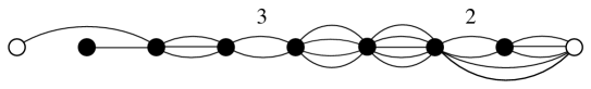
$\mathbf{r-l}=(1,1,1,0,1,0,0)$, $\mathbf{s}=(0,1,0,0,0,0,0)$

Figure 8. The floor diagram of Figure 7 with additional initial and final vertices.

Now remove all short edges from ${\mathcal{D}}^{\prime}$, that is, all edges of weight 1 between consecutive vertices. The result is an ordered collection of templates ${\bf\Gamma}=(\Gamma_{1},\dots,\Gamma_{m})$, listed left to right. We also keep track of the initial vertices $k_{1},\ldots,k_{m}$ of these templates.

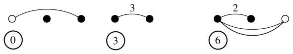
Figure 9. The template decomposition of the floor diagram of Figure 7.

Conversely, given the collection of templates ${\bf\Gamma}=(\Gamma_{1},\dots,\Gamma_{m})$, the starting points $k_{1},\ldots,k_{m}$, and the divergence sequence ${\bf a}=(d^{\,t},{\bf r}-{\bf l})$, this process is easily reversed. To recover ${\mathcal{D}}^{\prime}$, we first place the templates in their correct starting points in the interval $[1,\ldots,M]$, and draw in all the short edges that we removed from ${\mathcal{D}}^{\prime}$ from left to right. More precisely, to change the divergences from $a_{j}({\bf\Gamma})$ to $a_{j}$, we need to add $(a_{0}-a_{0}({\bf\Gamma}))+\cdots+(a_{j-1}-a_{j-1}({\bf\Gamma}))=(a_{0}+\cdots+a_{j-1}-\varkappa_{j}({\bf\Gamma}))$ short edges between $j-1$ and $j$. Finally, we remove the first and last vertices and their incident edges to obtain ${\mathcal{D}}$.

Given a divergence sequence ${\bf a}$ the possible starting points of the templates in a collection ${\bf\Gamma}=(\Gamma_{1},\dots,\Gamma_{m})$ are restricted by ${\bf a}$. More precisely, the valid sequences of starting points ${\bf k}=(k_{1},\dots,k_{m})$ of $\Gamma_{1},\dots,\Gamma_{m}$ are the ones in the set $A({{\bf\Gamma}},{\bf a})$ consisting of vectors ${\bf k}\in{\mathbb{N}}^{m}$ such that

• $k_{1}\geq 1-{\varepsilon}_{0}(\Gamma_{1})$,

• $k_{i+1}\geq k_{i}+l(\Gamma_{i})\quad\mbox{for all }i=1,\dots,m-1$,

• $k_{m}\leq M-l(\Gamma_{m})+{\varepsilon}_{1}(\Gamma_{m})$, and

• $a_{0}+\cdots+a_{k_{i}+j-1}-\varkappa_{j}(\Gamma_{i})\geq 0\quad\mbox{for }i=1,\dots,m,\mbox{ and }j=1,\dots,l(\Gamma_{i})$.

The first three inequalities guarantee that the templates fit in the interval $[1,\ldots,M]$ without overlapping. The last condition guarantees that the numbers of edges we need to add are non-negative. Notice that, for fixed ${\bf a}$, if $\delta({\mathcal{D}})=0$ (i.e., if ${\mathcal{D}}$ is the unique floor diagram with only short edges and $s_{i}=0$ for $i\geq 2$) then $A({\bf\Gamma},{\bf a})$ is empty as the decomposition removes all edges. Due to this abnormality we exclude the case $\delta=0$ in the sequel, though it is not hard to see that $N^{\Delta,0}=1$ for all $\Delta$.

We summarize the previous discussion in a proposition.

Proposition 3.2.

Let $M\geq 1$, and let ${\bf l},{\bf r}\in{\mathbb{Z}}^{M}$, ${\bf s}\in{\mathbb{N}}^{M}$. Let $d^{\,t}=s_{1}+\cdots+s_{M}$ and ${\bf a}=(d^{\,t},{\bf r}-{\bf l})$. The procedure of template decomposition is a bijection between the $({\bf l},{\bf r},{\bf s})$-floor diagrams and the pairs $({\bf\Gamma},{\bf k})$ of a collection of templates ${\bf\Gamma}$ and a valid sequence of starting points ${\bf k}\in A({\bf\Gamma},{\bf a})$.

3.3. Multiplicity, cogenus, and markings.

Now we show that the multiplicity, cogenus, and markings of a floor diagram behave well under template decomposition.

3.3.1. Multiplicity.

If a floor diagram ${\mathcal{D}}$ has template decomposition ${\bf\Gamma}$, then clearly

$$\mu({\mathcal{D}})=\prod_{i=1}^{m}\mu(\Gamma_{i}).$$

3.3.2. Cogenus.

Define the reversal sets ${\text{Rev}}({\bf r})$ of the sequences ${\bf r}$ and ${\bf l}$ by

$${\text{Rev}}({\bf r})=\{1\leq i<j\leq M:r_{i}<r_{j}\},\quad{\text{Rev}}({\bf l})=\{1\leq i<j\leq M:l_{i}>l_{j}\}.$$

The asymmetry is due to the fact that the “natural” order for ${\bf r}$ is the weakly decreasing one, while for ${\bf l}$ it is the weakly increasing one. Define the cogenus of the pair $({\bf l},{\bf r})$ as

$$\delta({\bf l},{\bf r})=\sum_{(i,j)\in{\text{Rev}}({\bf r})}(r_{j}-r_{i})\quad+\sum_{(i,j)\in{\text{Rev}}(-{\bf l})}(l_{i}-l_{j}).$$

Note that in the corresponding tropical curve, $(r_{j}-r_{i})+(l_{i}-l_{j})$ is the number of times that floors $i$ and $j$ cross, counted with multiplicity.

Given a collection of templates ${\bf\Gamma}=(\Gamma_{1},\dots,\Gamma_{m})$ we abbreviate the sum over their cogenera by $\delta({\bf\Gamma}):=\sum_{i=1}^{m}\delta(\Gamma_{i})$. The template decomposition is cogenus preserving, in the sense that

$$\delta({\mathcal{D}})=\delta({\bf\Gamma})+\delta({\bf l},{\bf r}).$$

This is because the tropical curve corresponding to ${\mathcal{D}}$ has $\delta({\mathcal{D}})$ nodes, counted with multiplicity; see Figure 2. The nodes arise in one of three ways: from an elevator crossing a floor, from an elevator with multiplicity greater than $1$, or from the crossing of two floors. There are exactly $\delta({\bf\Gamma})$ tropical nodes of the first two kinds and $\delta({\bf l},{\bf r})$ of the last kind, each counted with multiplicity.

3.3.3. Markings.

The number of markings of a floor diagram is also expressible in terms of the “number of markings of the templates”. The reason is simple: In Step 4 of Definition 2.4, where we need to linearly order $\tilde{{\mathcal{D}}}$, we can linearly order each template independently. We need to introduce some notation.

Let ${\mathcal{D}}$ be a floor diagram with divergence sequence ${\bf a}=(a_{0},\ldots,a_{M})=(d^{\,t},{\bf r}-{\bf l})$. For each template $\Gamma$ and each non-negative integer $k$ (for which (3.1) is non-negative for all $j$) let $\Gamma_{({\bf a},k)}$ denote the graph obtained from $\Gamma$ by first adding

(3.1) $$a_{0}+a_{1}+\cdots+a_{k+j-1}-\varkappa_{j}(\Gamma)$$

short edges connecting $j-1$ to $j$, for $1\leq j\leq l(\Gamma)$ (so that the vertices now have divergences $a_{k},\ldots,a_{k+l(\Gamma)}$), and then subdividing each edge of the resulting graph by introducing one new vertex for each edge. Let $P_{\Gamma}({\bf a},k)$ be the number of linear extensions (up to equivalence) of the vertex poset of the graph $\Gamma_{({\bf a},k)}$ extending the vertex order of $\Gamma$. Then

$$\nu({\mathcal{D}})=\prod_{i=1}^{m}P_{\Gamma_{i}}({\bf a},k_{i})=:P_{{\bf\Gamma}}({\bf a},{\bf k}).$$

3.4. Severi degrees in terms of templates.

With this machinery the Severi degree $N^{\Delta,\delta}$ can be computed solely in terms of templates. We conclude from Theorem 2.7, Proposition 3.2, and the previous observations in this section:

Proposition 3.3.

For any $h$-transverse polygon $\Delta$ and $\delta\geq 1$ the Severi degree $N^{\Delta,\delta}$ is given by

(Severi2) $$N^{\Delta,\delta}=\sum_{({\bf l},{\bf r})\,:\,\delta({\bf l},{\bf r})\leq\delta}\,\,\,\sum_{{\bf\Gamma}\,:\,\delta({\bf\Gamma})=\delta-\delta({\bf l},{\bf r})}\,\,\left(\prod_{i=1}^{m}\mu(\Gamma_{i})\sum_{{\bf k}\in A({\bf\Gamma},{\bf a})}P_{{\bf\Gamma}}({\bf a},{\bf k})\right)$$

where the first sum is over all permutations ${\bf l}=(l_{1},\dots,l_{M})$ and ${\bf r}=(r_{1},\dots,r_{M})$ of the left and right directions $D_{l}$ and $D_{r}$ of $\Delta$ with $\delta({\bf l},{\bf r})\leq\delta$, and the second sum is over collections of templates ${\bf\Gamma}$ of cogenus $\delta-\delta({\bf l},{\bf r})$. As before, we denote the upper edge length $d^{\,t}$ of $\Delta$ by $a_{0}$, and write $a_{i}=r_{i}-l_{i}$ for $1\leq i\leq M$.

(Severi2) improves (Severi1) by removing the unwieldy divergence condition on floor diagrams. However, eventual polynomiality is still far from clear.

4. Polynomiality of Severi degrees: the “first-quadrant” case

We will now use (Severi2) to prove our main theorem: the polynomiality of the Severi degrees for toric surfaces given by sufficiently large $h$-transverse polygons. We do this in two steps. In this section we carry out the proof in detail for the family of first-quadrant polygons. The proof of this special case exhibits essentially all the features of the general case, and has the advantage of a more transparent notation. In Section 5 we explain how the arguments in this section are easily adapted to the general case.

In turn, we will first prove polynomiality of the Severi degrees for a fixed toric surface and variable multidegree (Theorem 4.10). It will then be easy to extend this proof to also show polynomiality as a function of the surface (Theorem 4.11).

Notation 4.1.

We say that an $h$-transverse polygon $\Delta=\Delta({\bf c},{\bf d})$ is a first-quadrant polytope if ${\bf c}^{l}=\textbf{0}=(0,\ldots,0)$ and ${\bf c}^{r}\geq\textbf{0}$. We will then omit ${\bf c}^{l}$ and ${\bf d}^{l}$ from the notation and write $\Delta({\bf c},{\bf d})=\Delta({\bf c}^{r},(d^{\,t};{\bf d}^{r}))=\Delta((c_{1},\ldots,c_{n}),(d_{0};d_{1},\ldots,d_{n}))$. The corresponding floor diagrams have $M=d_{1}+\cdots+d_{n}$ vertices. The multisets of left and right directions, and upper edge length are

$$D_{l}=\{0,\dots,0\},\quad D_{r}=\{\underbrace{c_{1},\dots,c_{1}}_{d_{1}},\dots,\underbrace{c_{n},\dots,c_{n}}_{d_{n}}\},\quad d_{0}.$$

Then ${\bf l}=\textbf{0}$ and ${\bf a}=(d_{0},{\bf r})$. We write $\delta({\bf r})=\delta({\bf l},{\bf r})$. Notice the subtle distinction between ${\bf a}$ and ${\bf r}$, which will become more important in Section 5.

For example, Figure 10 shows the polygon $\Delta((1,0),(1;3,1))$ which has right directions $1$ and $0$ with respective lengths $3$ and $1$, and upper edge length equal to 1. Here $D_{r}=\{1,1,1,0\}$.

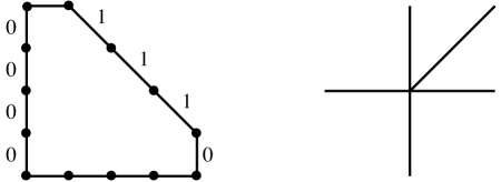
Figure 10. The first-quadrant polygon $\Delta((1,0),(1;3,1))$ and its normal fan.

Remark 4.2.

In this section we will assume that $\Delta({\bf c},{\bf d})$ is a first-quadrant $h$-transverse polygon. We will also assume that

$$d_{0}\geq\delta,\quad d_{0}+c_{1}\geq 2\delta,\quad d_{1},\ldots,d_{n}\geq\delta+1$$

and will simply say that ${\bf d}$ is large enough to describe these inequalities. Throughout most of the section we we will hold ${\bf c}$ constant and let ${\bf d}$ vary. (When we let ${\bf c}$ vary, we will say so explicitly.)

(Severi2) now reads:

(Severi2’) $$N^{\Delta,\delta}=\sum_{{\bf r}:\delta({\bf r})\leq\delta}\,\,\,\sum_{{\bf\Gamma}:\,\delta({\bf\Gamma})=\delta-\delta({\bf r})}\,\,\,\left(\prod_{i=1}^{m}\mu(\Gamma_{i})\sum_{{\bf k}\in A({\bf\Gamma},{\bf a})}P_{{\bf\Gamma}}({\bf a},{\bf k})\right)$$

To show that (Severi2’) yields an eventual polynomial in ${\bf c}$ and ${\bf d}$, our first problem is that the index set of the first sum is hard to control: as ${\bf c}$ and ${\bf d}$ vary, the index set of permutations ${\bf r}$ such that $\delta({\bf r})\leq\delta$ varies quite delicately with them. In particular, these permutations can be arbitrarily long. In turn, the index set of the second sum depends very sensitively on the value of $\delta({\bf r})$. These problems are solved by presenting a more compact encoding of ${\bf r}$.

4.1. From permutations to swaps.

Let us organize the permutations ${\bf r}$ of $D_{r}$ of cogenus less than or equal $\delta$ in a way which is uniform for large ${\bf c}$ and ${\bf d}$. Observe that, if ${\bf d}$ is large enough, then such a permutation cannot contain a reversal of $c_{i}$ and $c_{j}$ for $i\geq j+2$. This is because the minimum “divergence cost” of reversing $c_{i-1}$ and $c_{i+1}$ is $d_{i}\min\{c_{i}-c_{i+1},c_{i-1}-c_{i}\}\geq d_{i}>\delta$.

This observation allows us to encode such a permutation ${\bf r}$ into $n-1$ sequences of $1$s and $-1$s which, for each $1\leq i\leq n-1$, record the relative positions between the $c_{i}$s and the $c_{i+1}$s.

Example 4.3.

Suppose ${\bf c}=(5,3,2,1)$, ${\bf d}=(0,4,6,4,3)$, and ${\bf r}=55335353233212121$. This permutation decomposes into three sequences of $1$s and $-1$s as follows:

$$\begin{array}[]{ccccccccccccccccccc}{\bf a}&=&5&5&3&3&5&3&5&3&2&3&3&2&1&2&1&2&1\\ \\ 1&:&-1&-1&{\bf 1}&{\bf 1}&{\bf-}{\bf 1}&{\bf 1}&{\bf-}{\bf 1}&1&&1&1&&&&&&\\ 2&:&&&-1&-1&&-1&&-1&{\bf 1}&{\bf-}{\bf 1}&{\bf-}{\bf 1}&1&&1&&1&\\ 3&:&&&&&&&&&-1&&&-1&{\bf 1}&{\bf-}{\bf 1}&{\bf 1}&{\bf-}{\bf 1}&1\\ \end{array}\\$$

$$\pi_{1}=(1,1,-1,1,-1),\quad\pi_{2}=(1,-1,-1),\quad\pi_{3}=(1,-1,1,-1)$$

To achieve uniformity among different sequence lengths, we delete all initial $-1$s and all final $1$s in each such sequence. The result is a swap, which we define to be a sequence of $-1$s and $1$s which (is empty or) starts with a $1$ and ends with a $-1$.

We have encoded a permutation ${\bf r}$ into a sequence of $n-1$ swaps $\pi=(\pi_{1},\ldots,\pi_{n-1})$. Conversely, if we know ${\bf c}$ and ${\bf d}$ we can easily recover ${\bf r}=:\pi({\bf c},{\bf d})$ from $\pi$.

The following simple technical lemma will be crucial later, in the proof of Proposition 4.7.

Lemma 4.4.

Fix a collection ${\bf\pi}=(\pi_{1},\dots,\pi_{n-1})$ of swaps. Then, for ${\bf c}=(c_{1}>\cdots>c_{n})\in{\mathbb{Z}}_{>0}^{n}$, ${\bf d}=(d_{0};d_{1},\dots,d_{n})\in{\mathbb{Z}}_{\geq 0}^{n+1}$ and $0\leq t\leq\sum_{i=1}^{n}d_{i}$, the function (of ${\bf c}$, ${\bf d}$ and $t$)

$$a_{0}+a_{1}+\cdots+a_{t}=d_{0}+\pi({\bf c},{\bf d})_{1}+\cdots+\pi({\bf c},{\bf d})_{t}$$

is piecewise polynomial in ${\bf c}$, ${\bf d}$ and $t$ for large enough ${\bf d}$. Here ${\bf a}=(d_{0};{\bf r})=(d_{0},\pi({\bf c},{\bf d}))$. The regions of polynomiality are the faces of a hyperplane arrangement.

Proof.

Say $\pi_{i}$ contains $\alpha_{i}$ $1$s and $\beta_{i}$ $-1$s. We claim that, for large ${\bf d}$, the function $a_{0}+\cdots+a_{t}$ is polynomial when restricted to the lattice points in a fixed face of the following hyperplane arrangement in $({\bf c},{\bf d},t)$-space:

$$t=d_{1}+\cdots+d_{i}+f\qquad\textrm{ for }-\beta_{i}\leq f\leq\alpha_{i}\quad(1\leq i\leq n)$$

This is easy to see because

$${\bf a}=(d_{0},\pi({\bf c},{\bf d}))=(d_{0},\underbrace{c_{1},\ldots,c_{1}}_{d_{1}-\beta_{1}},\underbrace{c_{1}\textrm{s and }c_{2}\textrm{s}}_{\alpha_{1}+\beta_{1}},\underbrace{c_{2},\ldots,c_{2}}_{d_{2}-\alpha_{1}-\beta_{2}},\underbrace{c_{2}\textrm{s and }c_{3}\textrm{s}}_{\alpha_{2}+\beta_{2}},\underbrace{c_{3},\ldots,c_{3}}_{d_{3}-\alpha_{2}-\beta_{3}},\ldots)$$

where the order of the $c_{i}$s and $c_{i+1}$s is determined by $\pi$. Thus $a_{0}+a_{1}+\cdots+a_{t}$ equals

$$\begin{cases}d_{0}+tc_{1}&\textrm{ if }0\leq t\leq d_{1}-\beta_{1}\\ \quad d_{0}+tc_{1}+*&\quad\textrm{ if }t=d_{1}-\beta_{1}+1\\ \quad\quad\vdots&\quad\quad\vdots\\ \quad d_{0}+tc_{1}+*+\cdots+*&\quad\textrm{ if }t=d_{1}+\alpha_{1}-1\\ d_{0}+d_{1}c_{1}+(t-d_{1})c_{2}&\textrm{ if }d_{1}+\alpha_{1}\leq t\leq d_{1}+d_{2}-\beta_{2}\\ \quad d_{0}+d_{1}c_{1}+(t-d_{1})c_{2}+*&\quad\textrm{ if }t=d_{1}+d_{2}-\beta_{2}+1\\ \quad\quad\vdots&\quad\quad\vdots\\ \quad d_{0}+d_{1}c_{1}+(t-d_{1})c_{2}+*+\cdots+*&\quad\textrm{ if }t=d_{1}+d_{2}+\alpha_{1}-1\\ d_{0}+d_{1}c_{1}+d_{2}c_{2}+(t-d_{1}-d_{2})c_{3}&\textrm{ if }d_{1}+d_{2}+\alpha_{1}\leq t\leq d_{1}+d_{2}+d_{3}-\beta_{3}\\ \quad\vdots&\quad\vdots\end{cases}$$

where each $*$ represents a $c_{i}$ determined by $\pi$. The claim follows. ∎

Using the encoding of permutations into swaps, we now replace the first sum in (Severi2’) by a sum over swaps. Let the number of inversions ${\text{inv}}(\pi)$ of a swap $\pi$ be

$${\text{inv}}(\pi)=\#\{(i,j)\in{\mathbb{Z}}^{2}:1\leq i<j\leq n-1\text{ and }\pi(i)>\pi(j)\}.$$

It is easy to see that $\delta({\bf r})=\sum_{i=1}^{n-1}{\text{inv}}(\pi_{i})(c_{i}-c_{i+1})$. We obtain that, for large ${\bf d}$,

(Severi3’) $$N^{\Delta,\delta}=\sum_{{\bf\pi}}\,\,\sum_{{\bf\Gamma}:\,\,\delta({\bf\Gamma})=\delta-\delta({\bf r})}\quad\left(\prod_{i=1}^{m}\mu(\Gamma_{i})\sum_{{\bf k}\in A({\bf\Gamma},{\bf a})\cap{\mathbb{Z}}^{m}}P_{{\bf\Gamma}}({\bf a},{\bf k})\right)$$

where the first sum is now over all sequences ${\bf\pi}=(\pi_{1},\dots,\pi_{n-1})$ of swaps with $\sum_{i=1}^{n-1}{\text{inv}}(\pi_{i})(c_{i}-c_{i+1})\leq\delta$, ${\bf r}={\bf\pi}({\bf c},{\bf d})$, ${\bf a}=(d_{0},{\bf r})$ and the other sums are as before.

For fixed ${\bf c}$, the first sum in (Severi3’) is finite and its index set is independent of ${\bf d}$. Also, for each $\pi$ in that index set, $\delta({\bf r})$ is independent of ${\bf d}$, and hence so is the set of templates ${\bf\Gamma}$ in the second sum. The difficulty encountered in (Severi2’) is resolved.

If ${\bf c}$ is variable this observation still applies, under the additional assumption that ${\bf c}$ grows quickly enough that $c_{i}-c_{i+1}>\delta$ for all $i$. In that case, the first sum will only include the trivial swap sequence $\pi$ where every swap is empty, and then the index set of the second sum will still be independent of ${\bf d}$, and also of ${\bf c}$.

In (Severi3’) we have expressed $N^{\Delta,\delta}$ as a weighted sum of finitely many contributions of the form

$$N^{\Delta,\delta}_{\pi,{\bf\Gamma}}:=\sum_{{\bf k}\in A({\bf\Gamma},{\bf a})\cap{\mathbb{Z}}^{m}}P_{{\bf\Gamma}}({\bf a},{\bf k}),$$

where ${\bf a}=(d_{0},\pi({\bf c},{\bf d}))$. Our final goal is to show that, for fixed $\delta,{\bf\Gamma}$, and $\pi$, and for large ${\bf d}$, this function varies piecewise polynomially in ${\bf c}$ and ${\bf d}$. We will do it over the course of the Sections 4.2 – 4.5 by showing that $A({\bf\Gamma},{\bf a})$ is a variable polytope and $P_{{\bf\Gamma}}({\bf a},{\bf k})$ is piecewise polynomial, and then recurring to some facts about such discrete integrals.

4.2. Polytopality of $A(\Gamma,{\bf a})$.

Our next key proposition states that, for large enough ${\bf c}$ and ${\bf d}$, the innermost index set $A(\Gamma,{\bf a})\cap{\mathbb{Z}}^{m}$ of (Severi3’) is the set of lattice points in a polytope. While it does vary as a function of ${\bf d}$, it does so in a controlled way.

Proposition 4.5.

Let $\pi=(\pi_{1},\ldots,\pi_{n-1})$ be a fixed sequence of swaps and let    ${\bf\Gamma}=(\Gamma_{1},\dots,\Gamma_{m})$ be a fixed collection of templates. Let $(c_{1}>\cdots>c_{n})\in{\mathbb{Z}}_{\geq 0}^{n}$ and ${\bf d}=(d_{0};d_{1},\dots,d_{n})\in{\mathbb{Z}}_{\geq 0}^{n+1}$ be variable and assume that $d_{0}\geq\delta({\bf\Gamma})$, $d_{0}+c_{1}\geq 2\delta({\bf\Gamma})$. Let ${\bf a}=(d_{0},{\bf r})=(d_{0},\pi({\bf c},{\bf d}))$. Then $A({\bf\Gamma},{\bf a})$ is the set of lattice points in a polytope whose facet directions are fixed, and whose facet parameters are linear functions of $d_{0},\dots,d_{n}$.

Proof.

The only non-linear conditions defining $A({\bf\Gamma},{\bf a})$ are the inequalities

$$a_{0}+\cdots+a_{k_{i}+j-1}-\varkappa_{j}(\Gamma_{i})\geq 0.$$

for $i=1,\dots,m$ and $j=1,\dots,l(\Gamma_{i})$. We will show that, under these hypotheses, they hold “for free”. In fact, we will show the stronger statement $a_{0}+a_{1}-\varkappa_{j}(\Gamma_{i})\geq 0$. This implies all other inequalities (since all $a_{j}$ are non-negative) with the possible exception of $a_{0}-\varkappa_{1}(\Gamma_{1})\geq 0$ if $k_{1}=0,j=1$, which we deal with separately.

For every $i=1,\dots,m$ we have

$$\varkappa_{j}(\Gamma_{i})\leq\sum_{\stackrel{{\scriptstyle e}}{{r\to s}}}w(e)\leq 2\sum_{\stackrel{{\scriptstyle e}}{{r\to s}}}\bigg{[}(s-r)w(e)-1\bigg{]}=2\delta(\Gamma_{i})\leq 2\delta({\bf\Gamma}),$$

where the sums are over the edges of $\Gamma_{i}$. Therefore $\varkappa_{j}(\Gamma_{i})\leq d_{0}+c_{1}-2\delta({\bf r})$. Finally, from the definition of the cogenus $\delta({\bf r})$ it is clear that $\delta({\bf r})\geq c_{1}-r_{1}$. Therefore $\varkappa_{j}(\Gamma_{i})\leq d_{0}+r_{1}-\delta({\bf r})\leq a_{0}+a_{1}$ as desired, since $a_{0}=d_{0}$ and $a_{1}=r_{1}$.

Now we prove $a_{0}-\varkappa_{1}(\Gamma_{1})\geq 0$ for $k_{1}=0$ and $j=1$. If $k_{1}=0$ we must have ${\varepsilon}_{0}(\Gamma_{1})=1$, so all edges of $\Gamma_{1}$ adjacent to vertex $0$ have weight $1$ and there are no edges between $0$ and $1$. Thus, we have $\varkappa_{1}(\Gamma_{1})\leq\delta(\Gamma_{1})\leq\delta({\bf\Gamma})$, and from our assumption $\delta({\bf\Gamma})\leq d_{0}$ we conclude that $\varkappa_{1}(\Gamma_{1})\leq a_{0}$.

Finally notice that the facet directions are fixed, and the only non-constant facet parameter depends only on $M=d_{1}+\cdots+d_{n}$. ∎

Remark 4.6.

In a sense, the “real content” of the previous proof is the following statement: when $d_{0}\geq\delta$ and $d_{0}+c_{1}\geq 2\delta$, all templates can move between the first and last vertex of the floor diagram without obstruction.

4.3. Piecewise polynomiality of $P_{{\bf\Gamma}}({\bf a},{\bf k})$.

Proposition 4.7.

Let $\pi=(\pi_{1},\ldots,\pi_{n-1})$ be a fixed collection of swaps and let    ${\bf\Gamma}=(\Gamma_{1},\dots,\Gamma_{m})$ be a fixed collection of templates. Let ${\bf c}=(c_{1}>\cdots>c_{n})\in{\mathbb{Z}}_{>0}^{n}$ and ${\bf d}=(d_{0};d_{1},\dots,d_{n})\in{\mathbb{Z}}_{\geq 0}^{n+1}$ be variable and ${\bf a}=(d_{0},{\bf r})=(d_{0},\pi({\bf c},{\bf d}))$. Let ${\bf k}\in A({\bf\Gamma},{\bf a})\cap{\mathbb{Z}}^{m}$ be variable. Then the function $P_{{\bf\Gamma}}({\bf a},{\bf k})$ is piecewise polynomial in ${\bf c}$, ${\bf d}$ and ${\bf k}$. The domains of polynomiality are faces of a hyperplane arrangement.

Proof.

Recall that $P_{{\bf\Gamma}}({\bf a},{\bf k})=\prod_{i=1}^{m}P_{\Gamma_{i}}({\bf a},k_{i})$. Let $\Gamma=\Gamma_{i}$ be one of the templates in ${\bf\Gamma}$ and let $k=k_{i}$. By definition, $P_{\Gamma}({\bf a},k)$ is the number of linear extensions of the acyclic graph $\Gamma_{({\bf a},k)}$ extending the order of the template $\Gamma$. Recall how this graph $\Gamma_{({\bf a},k)}$ is obtained from $\Gamma$: we add in the right number of short edges to $\Gamma$ (more precisely, $a_{0}+\cdots+a_{k+j-1}-\varkappa_{j}$ edges between vertices $j-1$ and $j$) so that the resulting graph has divergences $a_{k},\ldots,a_{k+l(\Gamma)-1}$, and then we introduce a new vertex at the midpoint of each edge.

Such a linear extension on $\Gamma_{({\bf a},k)}$ can be constructed in two steps. In Step 1, we choose a linear order (modulo equivalence) of the graph formed by the vertices $0,\dots,l(\Gamma)$ of $\Gamma$ and the midpoint vertices coming from edges of $\Gamma$. In Step 2 we insert the midpoint vertices of the new edges of $\Gamma_{({\bf a},k)}$ into the linear order of Step 1. If $b_{j}$ is the number of vertices between $j-1$ and $j$ in the linear order of Step 1, there are

(4.1) $$\prod_{j=1}^{l}\binom{a_{0}+\cdots+a_{k+j-1}-\varkappa_{j}(\Gamma)+b_{j}}{b_{j}}$$

ways to insert those midpoints, up to equivalence.

Notice that the parameters $\varkappa_{j}(\Gamma)$ and $b_{j}$ are constants that depend only on $\Gamma$. Lemma 4.4 tells us that $a_{0}+\cdots+a_{k+j-1}$ is a piecewise polynomial in ${\bf c}$, ${\bf d}$ and $k$, and the proof describes the domains of polynomiality. This allows us to conclude that the expression of (4.1) is polynomial on each face of the hyperplane arrangement

$$k=d_{1}+\cdots+d_{i}+f,\qquad-\beta_{i}-l(\Gamma)+1\leq f\leq\alpha_{i},$$

for $1\leq i\leq n$, and thus $P_{{\bf\Gamma}}({\bf a},{\bf k})$ is polynomial on each face of the following arrangement ${\mathcal{A}}$ in $({\bf c},{\bf d},{\bf k})$-space:

$${\mathcal{A}}:\quad k_{s}=d_{1}+\cdots+d_{i}+f,\qquad-\beta_{i}-l(\Gamma_{s})+1\leq f\leq\alpha_{i},$$

for $1\leq i\leq n$ and $1\leq s\leq m$. ∎

4.4. Discrete integrals of polynomials over polytopes.

In Section 4.2 we showed that $A({\bf\Gamma},{\bf a})\cap{\mathbb{Z}}^{m}$ is the set of lattice points in a polytope with fixed facet directions, and whose facet parameters are linear functions of ${\bf d}$. Since this set only depends on ${\bf d}$, we relabel it $A({\bf\Gamma},{\bf d})\cap{\mathbb{Z}}^{m}$. In Section 4.3 we showed that $P_{{\bf\Gamma}}({\bf a},{\bf k})$ is a piecewise polynomial function of ${\bf c},{\bf d},$ and ${\bf k}$, whose domains of polynomiality are cut out by a hyperplane arrangement $\mathcal{A}$. The equations of this arrangement have fixed normal directions, and parameters which are linear functions of ${\bf d}$ and ${\bf k}$. It follows that

$$N^{\Delta,\delta}_{\pi,{\bf\Gamma}}=\sum_{F}\sum_{{\bf k}\in(A({\bf\Gamma},{\bf d})\cap F)^{o}\cap{\mathbb{Z}}^{m}}P^{F}_{{\bf\Gamma}}({\bf c},{\bf d},{\bf k}),$$

summing over the faces $F$ of $\mathcal{A}$, where each $P_{\bf\Gamma}^{F}$ is a polynomial. Here $Q^{o}$ denotes the relative interior of $Q$, i.e., the interior of $Q$ with respect to its affine span. We get:

(Severi4) $$N^{\Delta,\delta}=\sum_{\pi,{\bf\Gamma},F}\,\,\sum_{{\bf k}\in(A({\bf\Gamma},{\bf d})\cap F)^{o}\cap{\mathbb{Z}}^{m}}P^{F}_{{\bf\Gamma}}({\bf c},{\bf d},{\bf k}).$$

This is a somewhat messy expression, but the point is that there is a finite number of choices for $\pi,{\bf\Gamma},$ and $F$, and these choices are independent of ${\bf d}$. Now we just need to prove the polynomiality of the inner sum, which is a discrete integral of a polynomial function over a variable open polytope.

To do so, we invoke some results on discrete integrals. Given a polytope $Q\subset{\mathbb{R}}^{m}$ and a function $f:{\mathbb{R}}^{m}\rightarrow{\mathbb{R}}$, we define the discrete integral of $f$ over $Q$ to be

$$\sum_{q\in Q\cap{\mathbb{Z}}^{m}}f(q).$$

Recall that an $m$-polytope is simple if every vertex is contained in exactly $m$ edges. It is integral if all its vertices have integer coordinates. A facet translation of a polytope $P=\Pi_{X}({\bf y})=\{{\bf k}\in{\mathbb{R}}^{m}\,:\,X{\bf k}\leq{\bf y}\}$ is a polytope of the form $\Pi_{X}({\bf y}^{\prime})=\{{\bf k}\in{\mathbb{R}}^{m}\,:\,X{\bf k}\leq{\bf y}^{\prime}\}$ for ${\bf y}^{\prime}\in{\mathbb{R}}^{l}$, obtained by translating the facets of $P$. We assume that $X$ is an integer matrix and say $\Pi_{X}({\bf y}^{\prime})$ is an integer facet translation if ${\bf y}^{\prime}\in{\mathbb{Z}}^{l}$. Say that the matrix $X$ is unimodular, and that $P$ is facet-unimodular, if every maximal minor has determinant $-1,0,$ or $1$. When this is the case, every integer facet translation $\Pi_{X}({\bf y}^{\prime})$ has integral vertices by Cramer’s rule.

The values of ${\bf y}^{\prime}$ for which $\Pi_{X}({\bf y}^{\prime})$ and $P$ are combinatorially equivalent form an open cone in ${\mathbb{R}}^{m}$; its closure is the deformation cone of $P$. The corresponding polytopes are called deformations of $P$. [17, 18]

Recall that a quasipolynomial function on a lattice $\Lambda$ is a function which is polynomial on each coset of some finite index sublattice $\Lambda^{\prime}\subseteq\Lambda$. Results like the following are known, although we have not found in the literature the precise statement that we need:

Lemma 4.8.

Consider the integer facet translations of a simple rational polytope $P$ with fixed facet directions and variable facet parameters, i.e., the polytopes

$$\Pi_{X}({\bf y})=\{{\bf k}\in{\mathbb{R}}^{m}\,:\,X{\bf k}\leq{\bf y}\},$$

where $X\in{\mathbb{Z}}^{l\times m}$ is a fixed $l\times m$ matrix and ${\bf y}\in{\mathbb{Z}}^{l}$ is a variable vector. Let $f$ be a polynomial function and let

$$g({\bf y})=\sum_{{\bf k}\,\in\,\Pi_{X}({\bf y})\cap\,{\mathbb{Z}}^{m}}f({\bf k}),\qquad g^{o}({\bf y})=\sum_{{\bf k}\,\in\,\Pi_{X}({\bf y})^{o}\cap\,{\mathbb{Z}}^{m}}f({\bf k}).$$

be the discrete integrals of $f$ over $\Pi_{X}({\bf y})$, and over its relative interior. Then $g({\bf y})$ and $g^{o}({\bf y})$ are piecewise quasipolynomial functions of ${\bf y}$. The domains of quasipolynomiality are given by linear conditions in ${\bf y}$. More concretely, these functions are quasipolynomial when restricted to those ${\bf y}$ for which the polytope $\Pi_{X}({\bf y})$ has a fixed combinatorial type.
Furthermore, if $X$ is unimodular, then $g({\bf y})$ and $g^{o}({\bf y})$ are piecewise polynomial.

Proof.

This is certainly known for $f=1$, i.e., for the lattice point count $g({\bf y})=|\Pi_{X}({\bf y})\cap\,{\mathbb{Z}}^{m}|$. For instance, a proof can be found in [17, Theorem 19.3] for the parameters ${\bf y}$ for which $\Pi_{X}({\bf y})$ is integral. This proves the unimodular case, and is easily adapted to the non-unimodular case. That proof is easily modified to apply to any polynomial $f$. By subtracting off the boundary faces of our polytope (with alternating signs depending on the dimension) we obtain the results for $g^{o}$. ∎

Lemma 4.9.

Consider a variable polytope with fixed facet directions, and facet parameters which vary linearly as a function of a vector ${\bf d}$; i.e.,

$$\Pi_{X}(Y{\bf d})=\{{\bf k}\in{\mathbb{R}}^{m}\,:\,X{\bf k}\leq Y{\bf d}\}$$

where $X\in{\mathbb{Z}}^{l\times m}$ and $Y\in{\mathbb{Z}}^{l\times n}$ are fixed $l\times m$ and $l\times n$ matrices, and ${\bf d}\in{\mathbb{R}}^{n}$ is a variable vector. Let $f({\bf c},{\bf d},{\bf k})$ be a polynomial function of ${\bf c}\in{\mathbb{R}}^{n}$, ${\bf d}\in{\mathbb{R}}^{n}$, and ${\bf k}\in{\mathbb{R}}^{m}$, and let

$$g({\bf c},{\bf d})=\sum_{{\bf k}\,\in\,\Pi_{X}({\bf y})\cap\,{\mathbb{Z}}^{m}}f({\bf c},{\bf d},{\bf k}),\qquad g^{o}({\bf c},{\bf d})=\sum_{{\bf k}\,\in\,\Pi_{X}({\bf y})^{o}\cap\,{\mathbb{Z}}^{m}}f({\bf c},{\bf d},{\bf k}).$$

Then $g({\bf c},{\bf d})$ and $g^{o}({\bf c},{\bf d})$ are piecewise polynomial functions of ${\bf c}$ and ${\bf d}$. The domains of quasipolynomiality are given by linear conditions in ${\bf d}$. More concretely, these functions are quasipolynomial when restricted to those ${\bf d}$ for which the polytope $\Pi_{X}(Y{\bf d})$ has a fixed combinatorial type.
Furthermore, if $X$ is unimodular, then $g({\bf c},{\bf d})$ and $g^{o}({\bf c},{\bf d})$ are piecewise polynomial.

Proof.

This is an easy consequence of the previous lemma. Write $f({\bf c},{\bf d},{\bf k})=\sum_{\bf i}f_{\bf i}({\bf c},{\bf k}){\bf d}^{\bf i}$. By Lemma 4.8, $\sum_{{\bf k}\,\in\,\Pi_{X}({\bf y})\cap\,{\mathbb{Z}}^{m}}f_{\bf i}({\bf c},{\bf k})$ is a piecewise polynomial in $Y{\bf d}$, and therefore in ${\bf d}$, with polynomials in ${\bf c}$ as coefficients. The domains of polynomiality are given by linear conditions in $Y{\bf d}$, and hence in ${\bf d}$. Now sum over all ${\bf i}$ to obtain the desired result. ∎

4.5. Polynomiality of Severi degrees.

We are now ready to prove the eventual polynomiality of Severi degrees in the special case of first-quadrant polygons.

Theorem 4.10.

(Polynomiality of first-quadrant Severi degrees 1: Fixed Surface.)
Fix $n\geq 1$, $\delta\geq 1$, and ${\bf c}=(c_{1}>\cdots>c_{n})\in{\mathbb{Z}}^{n}$. There is a polynomial $p^{\bf c}_{\delta}({\bf d})$ such that the Severi degree $N_{{\mathrm{S}}({\bf c})}^{{\bf d},\delta}$ is given by

(4.2) $$N_{{\mathrm{S}}({\bf c})}^{{\bf d},\delta}=p^{\bf c}_{\delta}({\bf d})$$

for any ${\bf d}\in{\mathbb{Z}}_{\geq 0}^{n+1}$ such that $d_{0}\geq\delta$, $d_{0}+c_{1}\geq 2\delta$ and $d_{1},\ldots,d_{n}\geq\delta+1$.

Proof.

We do this in three steps.

Step 1. Piecewise quasipolynomiality. In (Severi4) there is a fixed (and finite) set of choices for $\pi,{\bf\Gamma}$, and $F$, independently of ${\bf d}$. For each such choice, the function $P^{F}_{{\bf\Gamma}}({\bf c},{\bf d},{\bf k})$ is polynomial in ${\bf c},{\bf d}$, and ${\bf k}$ (thanks to Section 4.3) and the domain $A({\bf\Gamma},{\bf d})\cap F$ is polytopal with fixed facet directions and facet parameters which are linear in ${\bf d}$ (thanks to Section 4.2). Lemma 4.9 then shows that $N^{\Delta,\delta}$ is piecewise quasipolynomial in ${\bf c}$ (which is constant here) and ${\bf d}$.

Step 2. Quasipolynomiality. To prove that all large ${\bf d}$ lie in the same domain of quasipolynomiality, we need to analyze those domains more carefully. Each polytope $A({\bf\Gamma},{\bf d})\cap F$ is the space of $(k_{1},\ldots,k_{m})$ such that

$$\begin{array}[]{rcll}k_{s}&\bigcirc&d_{1}+\cdots+d_{i}+f&(-\beta_{i}-l_{s}+1\leq f\leq\alpha_{i},\,\,1\leq i\leq n,\,\,1\leq s\leq m)\\ k_{1}&\geq&1-{\varepsilon}_{0}&\\ k_{s}-k_{s-1}&\geq&l_{s-1}&(2\leq s\leq m)\\ k_{m}&\leq&M-l_{m}+{\varepsilon}_{1},&\end{array}$$

where $\bigcirc$ represents $\geq,=$, or $\leq$, and we abbreviate $l_{i}:=l(\Gamma_{i}),{\varepsilon}_{0}:={\varepsilon}_{0}(\Gamma_{1})$ and ${\varepsilon}_{1}:={\varepsilon}_{1}(\Gamma_{m})$. We need to show that the combinatorial type of this polytope does not depend on ${\bf d}$.

Let’s examine how the parameters in ${\bf d}$ restrict the positions of the integers in ${\bf k}$ when ${\bf d}$ is large. The numbers $d_{1},d_{1}+d_{2},\ldots,d_{1}+\cdots+d_{n}=M$ are far from each other. The first set of inequalities “anchor” some of the $k_{s}$s to be very near the number $d_{1}+\cdots+d_{i}$. If $k_{s}$ is anchored near $d_{1}+\cdots+d_{i}$, then it is forced to equal $d_{1}+\cdots+d_{i}+f$, for some $f\in[-\beta_{i}-l_{s}+1,\alpha_{i}]$ which is determined by $F$ independently of ${\bf d}$. If $k_{s}$ is not anchored to any $d_{1}+\cdots+d_{i}$, then those inequalities allow it to roam freely inside one concrete large interval $[d_{1}+\cdots+d_{i},d_{1}+\cdots+d_{i+1}]$, but not too close to either endpoint of the interval.

Since ${\bf d}$ is large, the inequality $k_{s}-k_{s-1}\geq l_{s-1}$ is automatically satisfied by ${\bf k}$ unless one of three things happen:

• $k_{s-1}$ and $k_{s}$ are anchored to the same $d_{1}+\ldots+d_{i}$,

• neither is anchored, and both are restricted to lie in the same interval.

• one of them is anchored to $d_{1}+\cdots+d_{i}$, and the other one is restricted to one of the intervals adjacent to the same $d_{1}+\cdots+d_{i}$.

In the first case, either the inequality $k_{s}-k_{s-1}\geq l_{s-1}$ automatically holds (and does not define a facet of $A({\bf\Gamma},{\bf d})$) or it automatically does not hold (and the polytope is empty), depending on how far $k_{s-1}$ and $k_{s}$ are anchored from $d_{1}+\cdots+d_{i}$. In the second case, the inequality does not hold automatically, and therefore defines a facet of $A({\bf\Gamma},{\bf d})$. In the third case, the inequality may hold automatically (and not give a facet) or introduce a new restriction on ${\bf k}$ (and give a facet); but again, this depends only on the anchoring, and is independent of ${\bf d}$. A similar analysis holds for the inequalities $k_{1}\geq 1-{\varepsilon}_{0}$ and $k_{m}\leq M-l_{m}+{\varepsilon}_{1}$.

In summary, for large ${\bf d}$, the “shape” of the restrictions on ${\bf k}$ (i.e. the combinatorial type of $A({\bf\Gamma},{\bf d})\cap F$) is independent of ${\bf d}$. This proves that $N^{\Delta,\delta}$ is quasipolynomial for large ${\bf d}$.

Now we discuss the restrictions on ${\bf d}$ necessary for the previous analysis to hold. First, we need it to be impossible for $k_{s}$ to be anchored to $d_{1}+\cdots+d_{i}$ and to $d_{1}+\cdots+d_{i}+d_{i+1}$ simultaneously. This translates to $d_{1}+\cdots+d_{i+1}-\beta_{i+1}-l_{s}+1>d_{1}+\cdots+d_{i}+\alpha_{i}$, or $d_{i+1}\geq l(\pi_{i+1})+l_{s}$, for all $s$. We also need that, if $k_{s-1}$ is anchored to $d_{1}+\cdots+d_{i}$ and $k_{s}$ is anchored to $d_{1}+\cdots+d_{i+1}$, we automatically have $k_{s}-k_{s-1}\geq l_{s-1}.$ This requires the inequality $d_{1}+\cdots+d_{i+1}-\beta_{i+1}-l_{s}+1\geq d_{1}+\cdots+d_{i}+\alpha_{i}+l_{s}$, or $d_{i+1}\geq l(\pi_{i+1})+l_{s}+l_{s-1}-1$, which is stronger than the previous one. This last inequality follows from two easy observations: $l(\pi)\leq{\text{inv}}(\pi)+1$ for any swap $\pi$, and $l(\Gamma)\leq\delta(\Gamma)+1$ for all templates $\Gamma$. From these, and the assumption that ${\bf d}$ is large, we get

$$d_{i+1}\geq\delta+1=\delta({\bf r})+\delta(\Gamma)+1\geq{\text{inv}}(\pi)+l(\Gamma)\geq l(\pi)+l_{s}+l_{s-1}-1$$

as desired.

Step 3. Polynomiality. Finally, to prove polynomiality, we prove that the polytopes $A({\bf\Gamma},{\bf d})\cap F$ are facet-unimodular. This is easy since the rows of the matrix describing this polytope are of the form ${\bf e}_{i}$ or ${\bf e}_{i}-{\bf e}_{j}$, where ${\bf e}_{i}$ is the $i$th unit vector. This is a submatrix of the matrix of the root system $A_{m}=\{{\bf e}_{i}-{\bf e}_{j},\,1\leq i\neq j\leq m+1\}$, which is totally unimodular; i.e., all of its square submatrices have determinant $-1,0$, or $1$. [19] ∎

Theorem 4.11.

(Polynomiality of first-quadrant Severi degrees 2: Universality.)
Fix $n\geq 1$ and $\delta\geq 1$. There is a universal polynomial $p_{\delta}({\bf c},{\bf d})$ such that the Severi degree $N_{{\mathrm{S}}({\bf c})}^{{\bf d},\delta}$ is given by

(4.3) $$N_{{\mathrm{S}}({\bf c})}^{{\bf d},\delta}=p_{\delta}({\bf c},{\bf d}).$$

for any ${\bf c}=(c_{1}>\cdots>c_{n})\in{\mathbb{Z}}^{n}$ and ${\bf d}\in{\mathbb{Z}}_{\geq 0}^{n+1}$ such that $c_{i}-c_{i+1}\geq\delta+1$, $d_{i}\geq\delta+1$ for all $i$, $d_{0}\geq\delta$ and $d_{0}+c_{1}\geq 2\delta$.

Proof.

We have already done all the hard work, and this result follows immediately from the discussion at the end of Section 4.1. If $c_{i}-c_{i+1}>\delta$ for all $i$ then $\delta({\bf r})>\delta$ for any $\pi$ other than the trivial collection of empty swaps. Therefore, in this case (Severi3’) says

$$N^{\Delta,\delta}=\sum_{{\bf\Gamma}:\,\,\delta({\bf\Gamma})=\delta}\quad\left(\prod_{i=1}^{m}\mu(\Gamma_{i})\sum_{{\bf k}\in A({\bf\Gamma},{\bf a})\cap{\mathbb{Z}}^{m}}P_{{\bf\Gamma}}({\bf a},{\bf k})\right)$$

The indexing set for this sum no longer depends on ${\bf c}$, so this is simply a weighted sum of functions which are polynomial in ${\bf c}$ and ${\bf d}$ when ${\bf d}$ is large. The desired result follows. ∎

Remark 4.12.

This description gives, in principle, an explicit algorithm to compute the polynomial $p_{\delta}({\bf c},{\bf d})$. In Section 3 of [3], the second author describes an algorithm which generates all templates of a given cogenus. The discrete integral

$$\sum_{{\bf k}\in A({\bf\Gamma},{\bf a})\cap{\mathbb{Z}}^{m}}P_{{\bf\Gamma}}({\bf a},{\bf k})$$

can be evaluated symbolically by repeated application of Faulhaber’s formula ([3, Lemma 3.5], taken from [15]).

5. Polynomiality of Severi degrees: the general $h$-transverse case

We are now ready to prove our main results, Theorems 1.2 and 1.3, which assert the eventual polynomiality of the Severi degrees $N_{{\mathrm{S}}({\bf c})}^{{\bf d},\delta}$ for arbitrary $h$-transverse polygons. We simply adapt the proofs of Theorems 4.10 and 4.11 for first-quadrant polygons. The adaptation is fairly straightforward, though the details are slightly more cumbersome.

Remark 5.1.

In this section we assume that the $h$-transverse polygon $\Delta({\bf c},{\bf d})$ with ${\bf c}=({\bf c}^{r};{\bf c}^{l})$ and ${\bf d}=(d^{\,t};{\bf d}^{r};{\bf d}^{l})$ satisfies:

$$d^{\,t},d^{\,b}\geq\delta,\quad d^{\,t}+c^{r}_{1}-c^{l}_{1},d^{\,b}+c^{r}_{n}-c^{l}_{m}\geq 2\delta,\quad d^{\,r}_{1},\ldots,d^{\,r}_{n},d^{\,l}_{1},\ldots,d^{\,l}_{m}\geq\delta+1,$$

and

$$\left|(d^{\,r}_{1}+\ldots+d^{\,r}_{i})-(d^{\,l}_{1}+\ldots+d^{\,l}_{j})\right|\geq\delta+2\quad\textrm{ for }1\leq i\leq n-1,\,\,1\leq j\leq m-1$$

Proof of Theorem 1.2.

We follow the steps of Section 4 one at a time.

1. Swaps. The encoding of divergence sequences in terms of swaps still works, since ${\bf d}^{r}$ and ${\bf d}^{l}$ are large enough. Now we obtain two swap sequences $\pi^{r}$ and $\pi^{l}$ for ${\bf r}$ and ${\bf l}$, respectively. Here ${\bf a}=(d^{\,t},{\bf r}-{\bf l})$ where ${\bf r}-{\bf l}=\pi^{r}({\bf c}^{r},{\bf d}^{r})-\pi^{l}({\bf c}^{l},{\bf d}^{l})$, and the expression $a_{0}+\ldots+a_{t}$ is still piecewise polynomial in ${\bf c},{\bf d}$ and $t$. The regions of polynomiality are given by how far $t$ is from the numbers $d^{\,r}_{1}+\cdots+d^{\,r}_{i}$ (as before) and $d^{\,l}_{1}+\cdots+d^{\,l}_{j}$.

2. Polytopality. The domain $A({\bf\Gamma},{\bf a})$ of possible template starting points is still polytopal. To see this, once again, we prove that the potentially non-linear inequalities $a_{0}+\cdots+a_{{k_{i}}+j-1}\geq\varkappa_{j}(\Gamma_{i})$ hold automatically, by proving that:

$\bullet$ $a_{0}+\cdots+a_{m}\geq 2\delta({\bf\Gamma})$, for $1\leq m\leq M-1$ (and recalling that $2\delta({\bf\Gamma})\geq\varkappa_{j}(\Gamma_{i}$)),

$\bullet$ $a_{0}\geq\delta({\bf\Gamma})$ (which is needed if $k_{1}=0$ and ${\varepsilon}_{0}(\Gamma_{1})=1$)

$\bullet$ $a_{0}+\cdots+a_{M}\geq\delta({\bf\Gamma})$ (which is needed if $k_{m}=M-l(\Gamma_{m})+1$ and ${\varepsilon}_{1}(\Gamma_{m})=1$).

We need a different argument now since ${\bf a}$ is no longer non-negative.

Let $(\alpha_{0},\ldots,\alpha_{M})$ be the divergence sequence for $\Delta({\bf c},{\bf d})$ corresponding to the “natural” orders of $D_{l}$ and $D_{r}$: weakly decreasing for $D_{r}$ and weakly increasing for $D_{l}$. The sequence of partial sums $\alpha_{0}+\cdots+\alpha_{m}$ is unimodal. Therefore, for $1\leq m\leq M-1$,

$$\alpha_{0}+\cdots+\alpha_{m} \geq \min\{\alpha_{0}+\alpha_{1},\alpha_{0}+\cdots+\alpha_{M-1}\}$$

$$= \min\{d^{\,t}+c^{r}_{1}-c^{l}_{1},d^{\,b}+c^{r}_{n}-c^{l}_{m}\}\geq 2\delta.$$

Now observe that the difference $(\alpha_{0}+\cdots+\alpha_{m})-(a_{0}+\cdots+a_{m})$ is naturally a sum of terms $(r_{j}-r_{i})$ (where $(i,j)$ is a reversal of ${\bf r}$) and $(l_{i}-l_{j})$ (where $(i,j)$ is a reversal of $-{\bf l}$). Therefore $(\alpha_{0}+\cdots+\alpha_{m})-(a_{0}+\cdots+a_{m})\leq\delta({\bf l},{\bf r})$. It follows that, for $1\leq m\leq M-1$,

$$a_{0}+\cdots+a_{m}\geq(\alpha_{0}+\cdots+\alpha_{m})-\delta({\bf l},{\bf r})\geq 2\delta-\delta({\bf l},{\bf r})=\delta+\delta({\bf\Gamma})\geq 2\delta({\bf\Gamma}).$$

proving the first series of inequalities.

The second and third inequality follow from our assumptions since $a_{0}=d^{\,t}$ and $a_{0}+\cdots+a_{M}=d^{\,b}$.

3. Piecewise polynomiality. The results of Section 4.4 hold in exactly the same way for ${\bf a}={\bf r}-{\bf l}=\pi^{r}({\bf c}^{r},{\bf d}^{r})-\pi^{l}({\bf c}^{l},{\bf d}^{l})$. The only difference is that, as in Step 1 above, the domains of polynomiality now are given by how far $k_{s}$ is from the numbers $d^{\,r}_{1}+\cdots+d^{\,r}_{t}$ (as before) and $d^{\,l}_{1}+\cdots+d^{\,l}_{t}$.

4. Discrete integrals over polytopes. Section 4.4 holds without any changes.

5. Polynomiality of Severi degrees. To prove Theorem 4.10 for general $h$-transversal polygons, the only adjustment we have to make is in the argument for quasipolynomiality (Step 2 of that proof). In this context, the $k_{s}$s can be anchored near the numbers $d^{\,r}_{1}+\cdots+d^{\,r}_{t}$ and $d^{\,l}_{1}+\cdots+d^{\,l}_{t}$, and we have to ensure that these anchor points are sufficiently far from each other. The exact same argument works if we assume that $|(d^{\,r}_{1}+\ldots+d^{\,r}_{i})-(d^{\,l}_{1}+\ldots+d^{\,l}_{j})|\geq\delta+2$. We now need to impose a bound of $\delta+2$ instead of $\delta+1$ because we apply the inequality $l(\pi)\leq\textrm{inv}(\pi)+1$ twice: for $\pi=\pi^{r}$ and $\pi=\pi^{l}$. ∎

Proof of Theorem 1.3.

In Step 1 above, notice that if ${\bf c}$ is such that $c^{r}_{i}-c^{r}_{i+1}>\delta$ and $c^{r}_{j}-c^{r}_{j+1}>\delta$, then $\pi^{r}$ and $\pi^{l}$ must be empty. Therefore the proof of Theorem 4.11 applies here as well. ∎

Remark 5.2.

So far, our polynomiality results on Severi degrees are stated only for toric surfaces arising from polygons with two sufficiently long horizontal edges, due to the assumptions $d^{\,t}\geq\delta$ and $d^{\,b}\geq\delta$. In particular, this excludes the surface ${\mathbb{C}}{\mathbb{P}}^{2}$.

By a slight modification of our argument one can show that there exist universal polynomials for the families of Severi varieties of toric surfaces associated to lattice polygons with only one or no horizontal edge. More precisely, by setting one or both of the numbers $d^{\,t}$ and $d^{\,b}$ to $0$, one can show a universal polynomiality theorem analogous to Theorem 1.3, with the conditions $d^{\,t}\geq\delta$ and/or $d^{\,b}\geq\delta$ removed when appropriate. A proof of this variation can be obtained from our argument by, in essence, disregarding the terms ${\varepsilon}_{0}(\Gamma_{1})$ and/or ${\varepsilon}_{1}(\Gamma_{m})$ in the definition of the space $A({\bf\Gamma},{\bf a})$ of possible locations of the templates in a collection ${\bf\Gamma}$.

A priori, the universal polynomials in these alternate settings are different from the polynomials $p_{\delta}({\bf c},{\bf d})$ of Theorem 1.3. However, we expect that they should be closely related; their relationship should be further clarified.

6. Explicit computations

6.1. Hirzebruch Surfaces

Our results specialize as follows: For a non-negative integer $m$ let $F_{m}$ be the Hirzebruch surface associated to the convex hull of $(0,0)$, $(0,1)$, $(1,1)$ and $(m+1,0)$. In particular, $F_{0}={\mathbb{C}}{\mathbb{P}}^{1}\times{\mathbb{C}}{\mathbb{P}}^{1}$. Let $N^{(F_{m},{\mathcal{L}}_{m}(a,b)),\delta}$ be the degree of the Severi variety of $\delta$-nodal curves in $F_{m}$ with bi-degree $(a,b)$, i.e., of $\delta$-nodal curves whose Newton polygon is the convex hull of the points $(0,0)$, $(0,b)$, $(a,b)$ and $(a+bm,0)$.

Corollary 6.1.

(Polynomiality of Severi degrees for Hirzebruch Surfaces.) For fixed
$\delta\geq 0$, there exists a universal polynomial $p_{\delta}(a,b,m)$ such that the Severi degrees of Hirzebruch surfaces are given by

$$N^{(F_{m},{\mathcal{L}}_{m}(a,b)),\delta}=p_{\delta}(a,b,m)$$

for all positive integers $a,b,m$ with $a\geq\delta$, $a+m\geq 2\delta$ and $b\geq\delta+1$.

Proof.

Following the proof of Theorem 4.10 we find that in this case there are no swaps. Therefore the proof of Theorem 4.11 applies to this case. ∎

Remark 6.2.

The universal polynomials $p_{\delta}(a,b,m)$ for Hirzebruch surfaces $F_{m}$ for $\delta\leq 3$ are:

$$\tiny\begin{split}p_{0}(a,b,m)&=1,\\ p_{1}(a,b,m)&=3b^{2}m+6ab-2bm-4a-4b+4,\\ p_{2}(a,b,m)&=\frac{9}{2}b^{4}m^{2}+18ab^{3}m-6b^{3}m^{2}+18a^{2}b^{2}-24ab^{2}m-12b^{3}m+2b^{2}m^{2}-24a^{2}b-24ab^{2}+8abm-b^{2}m+8a^{2}\\ &-2ab+8b^{2}+\frac{23}{2}bm+23a+23b-30,\\ p_{3}(a,b,m)&=\frac{9}{2}b^{6}m^{3}+27ab^{5}m^{2}-9b^{5}m^{3}+54a^{2}b^{4}m-54ab^{4}m^{2}-18b^{5}m^{2}+6b^{4}m^{3}+36a^{3}b^{3}-108a^{2}b^{3}m-72ab^{4}m\\ &+36ab^{3}m^{2}-21b^{4}m^{2}-\frac{4}{3}b^{3}m^{3}-72a^{3}b^{2}-72a^{2}b^{3}+72a^{2}b^{2}m-84ab^{3}m-8ab^{2}m^{2}+24b^{4}m+\frac{137}{2}b^{3}m^{2}\\ &+48a^{3}b-84a^{2}b^{2}-16a^{2}bm+48ab^{3}+274ab^{2}m+137b^{3}m-31b^{2}m^{2}-\frac{32}{3}a^{3}+274a^{2}b+274ab^{2}-124abm\\ &-\frac{32}{3}b^{3}-68b^{2}m-124a^{2}-136ab-124b^{2}-\frac{374}{3}bm-\frac{748}{3}a-\frac{748}{3}b+452.\end{split}$$

Implicitly, for $0\leq\delta\leq 5$, the polynomials $p_{\delta}(a,b,m)$ are given by

$$\sum_{\delta\geq 0}p_{\delta}(a,b,m)x^{\delta}=\exp\Big{(}\sum_{\delta\geq 1}q_{\delta}(a,b,m)x^{\delta}\Big{)},$$

where

$$\begin{split}q_{1}(a,b,m)&=3(b^{2}m+2ab)-2(bm+2a+2b)+4,\\ q_{2}(a,b,m)&=\tfrac{1}{2}(-42(b^{2}m+2ab)+39(bm+2a+2b)-76),\\ q_{3}(a,b,m)&=\tfrac{1}{3}(690(b^{2}m+2ab)-788(bm+2a+2b)+1780),\\ q_{4}(a,b,m)&=\tfrac{1}{4}(-12060(b^{2}m+2ab)+15945(bm+2a+2b)-41048),\\ q_{5}(a,b,m)&=\tfrac{1}{5}(217728(b^{2}m+2ab)-321882(bm+2a+2b)+921864).\\ \end{split}$$

These were computed by a Maple implementation of the algorithm of Remark 4.12.

Remark 6.3.

An alternative way to compute the polynomials $p_{\delta}(a,b,m)$ for small $\delta$ is to use the Göttsche-Yau-Zaslow formula [12, Conjecture 2.4], recently proved by Tzeng [21]. This formula states that there exist universal power series $B_{1}(q)$ and $B_{2}(q)$ such that the Severi degrees $N^{\delta}(S,{\mathcal{L}})$ (i.e., the number of $\delta$-nodal curves in $|{\mathcal{L}}|$ through an appropriate number of general points) of any smooth surface $S$ and sufficiently ample line bundle ${\mathcal{L}}$ are given by the generating function

(6.1) $$\sum_{\delta\geq 0}N^{\delta}(S,{\mathcal{L}})(DG_{2}(\tau))^{\delta}=\frac{(DG_{2}(\tau)/q)^{\chi({\mathcal{L}})}B_{1}(q)^{K_{S}^{2}}B_{2}(q)^{{\mathcal{L}}K_{S}}}{(\Delta(\tau)D^{2}G_{2}(\tau)/q^{2})^{\chi({\mathcal{O}}_{S})/2}},$$

where $q=e^{2\pi i\tau}$, $G_{2}(\tau)=-\frac{1}{24}+\sum_{n>0}\left(\sum_{d|n}d\right)q^{n}$ denotes the second Eisenstein series, $D=q\frac{d}{d\,q}$, $\Delta(\tau)=q\prod_{k>0}(1-q^{k})^{24}$ is the Weierstrass $\Delta$-function, and ${\mathcal{O}}_{S}$ is the structure sheaf of $S$. The formulas $\chi({\mathcal{O}}_{S})=\frac{1}{12}(K_{S}^{2}+C_{2}(S))$ and $\chi({\mathcal{L}})=\frac{1}{2}({\mathcal{L}}^{2}-{\mathcal{L}}K_{S})+\frac{1}{12}(K_{S}^{2}+C_{2}(S))$ put everything in terms of the four numbers ${\mathcal{L}}^{2},{\mathcal{L}}K_{S},K_{S}^{2}$, and $C_{2}(S)$.

The formula above allows us to compute the polynomials $q_{\delta}(a,b,m)$ from the Chern classes $C_{2}(T_{F_{m}})$, $C_{1}({\mathcal{L}}_{m}(a,b))$, $C_{1}(K_{F_{m}})$ for the Hirzebruch surface $F_{m}$ and the line bundle ${\mathcal{L}}_{m}(a,b)$ determined by $a$ and $b$, together with the coefficients of $B_{1}$ and $B_{2}$ (if these are known). More specifically, the first $t$ coefficients of $B_{1}$ and $B_{2}$ determine the polynomials $q_{\delta}(a,b,m)$ for $\delta\leq t$ (and vice versa) for any $t\geq 1$. The second author rigorously established the first $14$ coefficients of $B_{1}$ and $B_{2}$, by computing the node polynomials for ${\mathbb{C}}{\mathbb{P}}^{2}$ for $\delta\leq 14$. This extended work of Kleiman and Piene [14] for $\delta\leq 8$ and confirmed the prediction of Göttsche [12]. Using this method, one can in principle compute the polynomials $p_{\delta}(a,b,m)$ and $q_{\delta}(a,b,m)$ for $\delta\leq 14$. We note, however, that the methods of this paper to compute $p_{\delta}(a,b,m)$ are less efficient than in the ${\mathbb{C}}{\mathbb{P}}^{2}$ case [3]. With the current computational limitations, we expect computability of $p_{\delta}(a,b,m)$ in feasible time only for $\delta\leq 7$ or $8$.

Remark 6.4.

As Hirzebruch surfaces $F_{m}$ are smooth for all $m\geq 0$ and the four numbers ${\mathcal{L}}^{2},{\mathcal{L}}K_{S},K_{S}^{2}$, and $C_{2}(T_{F_{m}})$ are polynomial in $a,b$, and $m$ in this case, the polynomiality result of Corollary 6.1 also follows (with a weaker threshold) from Tzeng’s proof [21, Theorem 1.1] of Göttsche’s Conjecture.

6.2. A non-smooth example

We now compute the node polynomials of a family of singular toric surfaces for $\delta=1$ and $\delta=2$. For positive integers $c,d_{0},d_{1}$ and $d_{2}$, let $\Delta(c;d_{0},d_{1},d_{2})$ be the convex hull of the points $(0,0)$, $(0,d_{1}+d_{2})$, $(d_{0},d_{1}+d_{2})$, $(d_{0}+d_{1}c,d_{2})$ and $(d_{0}+d_{1}c,0)$; see Figure 11. The corresponding toric surface $S(c)$ is singular whenever $c\geq 2$. The Severi degree $N^{(d_{0},d_{1},d_{2}),\delta}_{S(c)}$ counts $\delta$-nodal curves whose Newton polygon is $\Delta(c;d_{0},d_{1},d_{2})$.

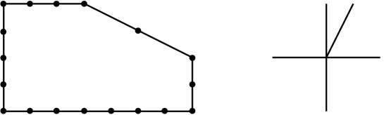
Figure 11. The convex hull of $(0,0),(0,d_{1}+d_{2}),(d_{0},d_{1}+d_{2}),\break(d_{0}+d_{1}c,d_{2})$, and $(d_{0}+d_{1}c,0))$, together with its normal fan. The cone dual to the vertex $(d_{0}+d_{1}c,d_{2})$ corresponds to a singular point of $S(c)$ if $c\geq 2$.

Corollary 6.5 (Polynomiality of Severi degrees for a non-smooth surface).

For fixed $\delta\geq 0$, there exists a universal polynomial $p_{\delta}(d_{0},d_{1},d_{2},c)$ such that

$$N^{(d_{0},d_{1},d_{2}),\delta}_{S(c)}=p_{\delta}(d_{0},d_{1},d_{2},c)$$

for all positive integers $d_{0},d_{1},d_{2},c$ with $d_{0}\geq\delta$, $d_{0}+c\geq 2\delta$, $d_{1},d_{2}\geq\delta$, $c\geq\delta+1$.

Proof.

Since $c\geq\delta+1$, there are no swaps and the proof of Theorem 4.11 applies. ∎

Remark 6.6.

Using the algorithm of Remark 4.12, we find that the universal polynomials $p_{\delta}(d_{0},d_{1},d_{2},c)$ for $\delta\leq 2$ are:

$$\tiny\begin{split}p_{0}(d_{0},d_{1},d_{2},c)=&1,\\ p_{1}(d_{0},d_{1},d_{2},c)=&3(d_{1}^{2}c+2d_{1}d_{2}c+2d_{0}d_{1}+2d_{0}d_{2})-2(d_{1}c+2d_{0}+2d_{1}+2d_{2})+4,\\ p_{2}(d_{0},d_{1},d_{2},c)=&\tfrac{9}{2}d_{1}^{4}c^{2}+18d_{1}^{3}d_{2}c^{2}+18d_{1}^{2}d_{2}^{2}c^{2}+18d_{0}d_{1}^{3}c+54d_{0}d_{1}^{2}d_{2}c+36d_{0}d_{1}d_{2}^{2}c-6d_{1}^{3}c^{2}-12d_{1}^{2}d_{2}c^{2}+18d_{0}^{2}d_{1}^{2}\\ &+36d_{0}^{2}d_{1}d_{2}+18d_{0}^{2}d_{2}^{2}-24d_{0}d_{1}^{2}c-36d_{0}d_{1}d_{2}c-12d_{1}^{3}c-36d_{1}^{2}d_{2}c+2d_{1}^{2}c^{2}-24d_{1}d_{2}^{2}c+2d_{1}d_{2}c^{2}\\ &-24d_{0}^{2}d_{1}-24d_{0}^{2}d_{2}-24d_{0}d_{1}^{2}-48d_{0}d_{1}d_{2}+8d_{0}d_{1}c-24d_{0}d_{2}^{2}+2d_{0}d_{2}c-d_{1}^{2}c-10d_{1}d_{2}c-2d_{1}c^{2}\\ &+8d_{0}^{2}-2d_{0}d_{1}-2d_{0}d_{2}-2d_{0}c+8d_{1}^{2}+16d_{1}d_{2}+\tfrac{23}{2}d_{1}c+8d_{2}^{2}+23d_{0}+23d_{1}+23d_{2}+4c-30.\end{split}$$

Equivalently, the polynomials $p_{\delta}(d_{0},d_{1},d_{2},c)$, for $\delta\leq 2$, are given by

$$\sum_{\delta\geq 0}p_{\delta}(d_{0},d_{1},d_{2},c)x^{\delta}=\exp\Big{(}\sum_{\delta\geq 1}q_{\delta}(d_{0},d_{1},d_{2},c)x^{\delta}\Big{)},$$

where

$$\begin{split}q_{1}(d_{0},d_{1},d_{2},c)=&3(d_{1}^{2}c+2d_{1}d_{2}c+2d_{0}d_{1}+2d_{0}d_{2})+2(-d_{1}c-2d_{0}-2d_{1}-2d_{2})+4,\\ q_{2}(d_{0},d_{1},d_{2},c)=&-42(d_{1}^{2}c+2d_{1}d_{2}c+2d_{0}d_{1}+2d_{0}d_{2})-39(-d_{1}c-2d_{0}-2d_{1}-2d_{2})\\ &+4(d_{1}c+d_{0})(d_{2}-1)c+8c-76.\end{split}$$

Let $T_{\delta}(w,x,y,z)$ be Göttsche’s universal polynomials for the smooth case (c.f.  Section 1.3), and define polynomials $Q_{\delta}(w,x,y,z)$ via

$$\sum_{\delta\geq 1}T_{\delta}(w,x,y,z)t^{\delta}=\exp\left(\sum_{\delta\geq 1}Q_{\delta}(w,x,y,z)t^{\delta}\right).$$

According to the Göttsche-Yau-Zaslow formula (6.1), the polynomials $Q_{\delta}(w,x,y,z)$ satisfy, for $\delta\leq 2$,

$$\begin{split}Q_{1}({\mathcal{L}}^{2},{\mathcal{L}}K_{S},K_{S}^{2},c_{2}(S))=&\,3{\mathcal{L}}^{2}+2{\mathcal{L}}K_{S}+c_{2}(S),\\ Q_{2}({\mathcal{L}}^{2},{\mathcal{L}}K_{S},K_{S}^{2},c_{2}(S))=&-42{\mathcal{L}}^{2}-39{\mathcal{L}}K_{S}-6K_{S}^{2}-7c_{2}(S).\\ \end{split}$$

If Göttsche’s conjecture held in this non-smooth example, we would have $Q_{1}=q_{1}$ and $Q_{2}=q_{2}$. For our example, we have

$$\begin{split}{\mathcal{L}}^{2}&=d_{1}^{2}c+2d_{1}d_{2}c+2d_{0}d_{1}+2d_{0}d_{2},\\ {\mathcal{L}}\cdot K_{S}&=-(d_{1}c+2d_{0}+2d_{1}+2d_{2}),\\ c_{2}^{\text{MP}}&=5,\\ K_{S}^{2}&=8-c\end{split}$$

where the first two computations are in the singular cohomology of the toric variety $S(c)$ ([6, Theorem 12.4.1]), and $c_{2}^{MP}$ is MacPherson’s Chern class as computed in [1]. Then we get

$$\begin{split}Q_{1}=&\,3(d_{1}^{2}c+2d_{1}d_{2}c+2d_{0}d_{1}+2d_{0}d_{2})+2(-d_{1}c-2d_{0}-2d_{1}-2d_{2})+5,\\ Q_{2}=&-42(d_{1}^{2}c+2d_{1}d_{2}c+2d_{0}d_{1}+2d_{0}d_{2})-39(-d_{1}c-2d_{0}-2d_{1}-2d_{2})+6c-83.\end{split}$$

These expressions for $Q_{1}$ and $Q_{2}$ bear some similarity with the correct expressions for $q_{1}$ and $q_{2}$ above, but they do not coincide; so Göttsche’s formula for the smooth case does not apply to this surface. However, this example seems to suggest that some modification of Göttsche’s formula should still apply to a more general family of surfaces. We do not know what that modification would look like.

7. Further directions and open problems

Our work suggests several directions of further research, some of which we have alluded to throughout the paper. We collect them here.

• As mentioned in Section 1 the relationship between our work and Göttsche’s Conjecture needs to be further clarified. Göttsche’s Conjecture is stated for smooth surfaces, while the surfaces we consider are generally not smooth. Is there a common generalization?

• We suspect that Severi degrees of any large toric surface are universally polynomial, even though we have only been able to prove it for large $h$-transverse toric surfaces. This restriction comes from Brugallé and Mikhalkin’s observation that the encoding of tropical curves into floor diagrams only works in the $h$-transverse case. Can we adjust the definition of a floor diagram, or find a different combinatorial encoding that allows us to drop this restriction? This could involve making a different choice for our generic collection of points of Section 2.1.

• It should be possible to weaken the conditions on ${\bf c}$ and ${\bf d}$ in Theorems 1.2 and Theorem 1.3. It is possible that we can drop the conditions on ${\bf c}$ entirely; some conditions on ${\bf d}$ are surely necessary.

• It would be of interest, and probably within reach, to clarify how the polynomials $p_{\delta}({\bf c},{\bf d})$ vary when we drop horizontal edges from $\Delta$, or when we vary the lengths $m$ and $n$ of their input.

References

- [1] G. Barthel, J.-P. Brasselet, and K.-H. Fieseler, Classes de Chern des variétés toriques singulières, C. R. Acad. Sci. Paris Sér. I Math. 315 (1992), no. 2, 187–192.
- [2] D. N. Bernstein, The number of roots of a system of equations, Funkcional. Anal. i Priložen. 9 (1975), no. 3, 1–4.
- [3] F. Block, Computing node polynomials for plane curves, Math. Res. Lett. 18 (2011), 621–643.
- [4] E. Brugallé and G. Mikhalkin, Enumeration of curves via floor diagrams, C. R. Math. Acad. Sci. Paris 345 (2007), no. 6, 329–334.
- [5] by same author, Floor decompositions of tropical curves: the planar case, Proceedings of Gökova Geometry-Topology Conference 2008, Gökova Geometry/Topology Conference (GGT), Gökova, 2009, pp. 64–90.
- [6] D. Cox, J. Little, and H. Schenck, Toric varieties, Graduate Studies in Mathematics, vol. 124, American Mathematical Society.
- [7] P. Di Francesco and C. Itzykson, Quantum intersection rings, The moduli space of curves (Texel Island, 1994), Progr. Math., vol. 129, Birkhäuser Boston, Boston, MA, 1995, pp. 81–148.
- [8] F. Enriques, Sui moduli d’una classe di superficie e sul teorema d’esistenza per funzioni algebriche di due variabilis, Atti Accad. Sci. Torino 47 (1912).
- [9] S. Fomin and G. Mikhalkin, Labeled floor diagrams for plane curves, J. Eur. Math. Soc. (JEMS) 12 (2010), no. 6, 1453–1496.
- [10] W. Fulton, Introduction to intersection theory in algebraic geometry, CBMS Regional Conference Series in Mathematics, vol. 54, Published for the Conference Board of the Mathematical Sciences, Washington, DC, 1984.
- [11] by same author, Introduction to toric varieties, Annals of Mathematics Studies, vol. 131, Princeton University Press, Princeton, NJ, 1993, The William H. Roever Lectures in Geometry.
- [12] L. Göttsche, A conjectural generating function for numbers of curves on surfaces, Comm. Math. Phys. 196 (1998), no. 3, 523–533.
- [13] J. Harris, On the Severi problem, Invent. Math. 84 (1986), no. 3, 445–461.
- [14] S. Kleiman and R. Piene, Node polynomials for families: methods and applications, Math. Nachr. 271 (2004), 69–90.
- [15] D. Knuth, Johann Faulhaber and sums of powers, Math. Comp. 61 (1993), no. 203, 277–294.
- [16] R. D. MacPherson, Chern classes for singular algebraic varieties, Ann. of Math. (2) 100 (1974), 423–432.
- [17] A. Postnikov, Permutohedra, associahedra, and beyond, Int. Math. Res. Notices (2009), 1026–1106.
- [18] A. Postnikov, V. Reiner, and L. Williams, Faces of generalized permutohedra, Documenta Math. 13 (2008), 207–273.
- [19] A. Schrijver, Theory of linear and integer programming, Wiley-Interscience Series in Discrete Mathematics, John Wiley & Sons Ltd., Chichester, 1986, A Wiley-Interscience Publication.
- [20] F. Severi, Vorlesungen über Algebraische Geometrie, Teubner, Leipzig, 1921.
- [21] Y.-J. Tzeng, A proof of Göttsche-Yau-Zaslow formula, Preprint, arXiv:1009.5371, 2010.