hep-th/yymmnn

December 2010

One-loop corrections to the Nielsen-Olesen vortex: collective oscillations.

Jürgen Baacke

Fakultät Physik, Technische Universität Dortmund

D - 44221 Dortmund, Germany

Abstract

We connect the translation modes of the instanton in the two-dimensional Abelian Higgs model with local translations of the vortex of the related model in (3+1) dimensions, the Nielsen-Olesen vortex. In this context these modes describe collective oscillations of the string. We construct the wave function of this mode and we derive, via a virial theorem, an effective action for these oscillations, which is consistent with the action constructed by Nielsen and Olesen using general arguments. We discuss some aspects of renormalization, based on a recent computation of one loop corrections to string tension of the vortex.

1 Introduction

A long time ago Nielsen and Olesen [1] discussed the vortex solution of the (3+1) dimensional Abelian Higgs model as a possible model for strings. In the same publication the authors discuss the effective action for the transverse collective oscillations of the vortex which they find to be equivalent to the Nambu-Goto action of string theory (see e.g. [2]). Their derivation is based on a general consideration of Lorentz transformation properties of such oscillations. We here derive the nonrelativistic limit of this effective action from an analysis of the fluctuations in the underlying quantum field theory.

For quantum kinks (see, e.g., [3, 4]) the collective motion is related to the translation mode. It is generated by infinitesimal displacements of the classical kink solution and is a zero mode of the fluctuation operator. Its quantization requires a special approach, by which the zero mode is found to carry the kinetic energy of the collective motion of the kink.

In the Abelian Higgs model in two dimensions one finds an instanton solution which describes topological transitions [5]. The fluctuations around the classical solution display two zero modes which again are related to translation invariance. The one-loop prefactor for the semiclassical transition rate is related to the functional determinant of the fluctuation operator. The zero modes would cause this determinant to be infinite and have to be eliminated. If handled properly, this elimination produces the correct dimension for the transition rate [6, 7].

The instanton of the Abelian Higgs model reappears in the $(3+1)$ dimensional version of the model as the vortex solution which we will consider here. The vortex solution is identical to the instanton solution in the transversal $x$ and $y$ coordinates, and it is independent on $z$ and of time. The translation of the classical solution now becomes local, dependent on $z$. Instead of a collective motion of a quantum kink we have collective oscillations of the vortex. The pole at $p_{\perp}=0$ in the Euclidian Green’s function of the two-dimensional model becomes a cut in the Green’ s function of the model in four dimensions. In the computation of one-loop corrections to the string tension [8] these modes can be included in the same way as all other fluctuations, in contrast to the two-dimensional case. Indeed, for the renormalization of these corrections it is necessary to include the zero mode contribution. Still the translation modes play a special rôle, and in the present work we will discuss these particular aspects.

The text is organized as follows: In Sec. 2 we present the model, the classical vortex solution and the classical string tension. In Sec. 3 we define the fluctuation operator and relate it to the one-loop correction to the string tension. Based on the derivation of the translation mode wave functions in Appendix A and using a virial theorem proven in Appendix B we discuss in Sec. 4 the collective string oscillations and their effective action. We discuss in Sec. 5 the rôle of the zero modes in the computation of the renormalized the string tension. Conclusions are presented in Sec. 6.

2 Basic relations

The Abelian Higgs model in (3+1) dimensions is defined by the Lagrange density

$${\cal L}=-\frac{1}{4}F_{\mu\nu}F^{\mu\nu}+\frac{1}{2}(D_{\mu}\phi)^{*}D^{\mu}\phi-\frac{\lambda}{4}\left(|\phi|^{2}-v^{2}\right)^{2}\;.$$ (2.1)

Here $\phi$ is a complex scalar field and

$$F_{\mu\nu} = \partial_{\mu}A_{\nu}-\partial_{\nu}A_{\mu}\;,$$ (2.2)

$$D_{\mu} = \partial_{\mu}-igA_{\mu}\;.$$ (2.3)

The particle spectrum consists of Higgs bosons of mass $m_{H}^{2}=2\lambda v^{2}$ and vector bosons of mass $m_{W}^{2}=g^{2}v^{2}$. The model allows for vortex type solutions, representing strings with a magnetic flux, the Nielsen-Olesen vortices [9, 1, 10]. The cylindrically symmetric ansatz for this solution is given, in the singular gauge, by

$$A^{{\rm cl}\perp}_{i}(x,y,z) = \frac{\varepsilon_{ij}x^{\perp}_{j}}{gr^{2}}\left[A(r)+1\right]\;\;\;i=1,2$$ (2.4)

$$\phi^{cl}(x,y,z) = vf(r)\;.$$ (2.5)

where $r=\sqrt{x^{2}+y^{2}}$ and $\varphi$ is the polar angle. Furthermore $A_{3}^{\rm cl}=A_{0}^{\rm cl}=0$. With this ansatz the energy per unit length, or string tension $\sigma$ takes the form

$$\sigma_{\rm cl} = \pi v^{2}\int^{\infty}_{0}\!\!\!dr\left\{\frac{1}{rm_{W}^{2}}\left[\frac{dA(r)}{dr}\right]^{2}\!\!+r\left[\frac{df(r)}{dr}\right]^{2}\!\!+\frac{f^{2}(r)}{r}\left[A(r)+1\right]^{2}\!\!\right.$$ (2.6)

$$+ \left.\frac{rm^{2}_{H}}{4}\left[f^{2}(r)-1\right]^{2}\!\right\}\;.$$

The classical equations of motion are given by

$$\left\{\frac{\partial^{2}}{\partial r^{2}}+\frac{1}{r}\frac{\partial}{\partial r}-\frac{\left[A(r)+1\right]^{2}}{r^{2}}-\frac{m^{2}_{H}}{2}\left[f^{2}(r)-1\right]\right\}f(r) = 0\;,$$ (2.7)

$$\left\{\frac{\partial^{2}}{\partial r^{2}}-\frac{1}{r}\frac{\partial}{\partial r}-m^{2}_{W}f^{2}(r)\right\}\left[A(r)+1\right] = 0\;,$$ (2.8)

which are to be solved numerically with

$$\begin{array}[]{rcccccr}A(r)&\stackrel{{\scriptstyle\scriptscriptstyle{r\to 0}}}{{\longrightarrow}}&{\rm const.}\cdot r^{2}&,&A(r)&\stackrel{{\scriptstyle\scriptscriptstyle{r\to\infty}}}{{\longrightarrow}}&-1\;,\\ f(r)&\stackrel{{\scriptstyle\scriptscriptstyle{r\to 0}}}{{\longrightarrow}}&{\rm const.}\cdot r&,&f(r)&\stackrel{{\scriptstyle\scriptscriptstyle{r\to\infty}}}{{\longrightarrow}}&1\;,\end{array}\;.$$ (2.9)

3 Fluctuation operator and one-loop string tension

Expanding the gauge and Higgs fields as

$$\phi = \phi_{i}^{\rm cl}+\varphi_{1}+i\varphi_{2}$$ (3.10)

$$A_{\mu} = A_{\mu}^{\rm cl}+a_{\mu}$$ (3.11)

the dynamics of the fluctuations is described by the second order gauge fixed Lagrangian [6]

$${\cal L}^{II} = -a_{\mu}\frac{1}{2}\left(-\Box-g^{2}\phi^{2}\right)a^{\mu}$$

$$+\varphi_{1}\frac{1}{2}\left[-\Box+g^{2}A_{\mu}A^{\mu}-\lambda\left(3\phi^{2}-v^{2}\right)\right]\varphi_{1}$$

$$+\,\varphi_{2}\frac{1}{2}\left[-\Box+g^{2}A_{\mu}A^{\mu}-g^{2}\phi^{2}-\lambda\left(\phi^{2}-v^{2}\right)\right]\varphi_{2}$$

$$+\,\varphi_{2}(gA^{\mu}\partial_{\mu})\varphi_{1}+\varphi_{1}(-gA^{\mu}\partial_{\mu})\varphi_{2}$$

$$+\,a^{\mu}(2g^{2}A_{\mu}\phi)\varphi_{1}+\,a^{\mu}(2g\partial_{\mu}\phi)\varphi_{2}$$

$$+\eta_{1}\frac{1}{2}\left(-\Box-g^{2}\phi^{2}\right)\eta_{1}+\eta_{2}\frac{1}{2}\left(-\Box-g^{2}\phi^{2}\right)\eta_{2}\;,$$

Here $\varphi_{1}$ and $\varphi_{2}$ denote the real and imaginary part of the Higgs field fluctuations, $\eta_{i}$ are the Faddeev-Popov ghosts, and we have chosen the ’t Hooft-Feynman background gauge. In compact notation this may be written as

$${\cal L}^{II}=\frac{1}{2}\psi^{*}_{i}{\cal M}_{ij}\psi_{j}\;.$$ (3.13)

The fields $\psi_{i}$ denote the ensemble of gauge, Higgs and Faddeev-Popov fields and the fluctuation operator ${\cal M}_{ij}$ is defined by this and the previous equation. In terms of the fluctuation operators ${\cal M}$ on the vortex and ${\cal M}^{0}$ for the vacuum background fields, the effective action is defined as

$$S_{eff}=\frac{i}{2}\ln\left\{\frac{\det{\cal M}+i\epsilon}{\det{\cal M}^{0}+i\epsilon}\right\}\;.$$ (3.14)

As the background field is time-independent and also independent of $z$ the fluctuation operators take the form

$${\cal M}_{ij}=(\partial_{0}^{2}-\partial_{3}^{2})\delta_{ij}+{\cal M}_{\perp ij}\;,$$ (3.15)

where ${\cal M}_{\perp}$ is a positive-definite operator describing the transversal fluctuations. It is identical for the longitudinal and timelike gauge fields and for the Faddeev-Popov ghosts, so these contributions to the effective action cancel. The remaining degrees of freedom form a coupled system of four fields $\psi_{i}$: the real and imaginary part of the Higgs field fluctuations $\varphi_{1},\varphi_{2}$ and the transverse gauge field fluctuations $a_{1},a_{2}$.

As is well known the logarithm of the determinant can be written as the trace of the logarithm. One can do the trace over $k_{0}$, the momentum associated with the time variable, by integrating over $T\int dk_{0}/2\pi$, where $T$ is the lapse of time. One then obtains

$$S_{\rm eff}=-T\frac{1}{2}\sum\left[E_{\alpha}-E_{\alpha}^{(0)}\right]\;,$$ (3.16)

where $E_{\alpha}$ are square roots of the eigenvalues of the positive definite operator

$$-\partial_{3}^{2}+{\cal M}_{\perp}\;,$$ (3.17)

and likewise $E_{\alpha}^{(0)}$ are those of the analogous operator in the vacuum

$$-\partial_{3}^{2}+{\cal M}_{\perp}^{0}=-\partial_{3}^{2}-\vec{\nabla}_{\perp}^{2}+{\bf m^{2}}\;.$$ (3.18)

Here ${\bf m}^{2}={\rm diag}(m_{1}^{2},\dots,m_{n}^{2})$ is the diagonal mass squared operator for the various fluctuations.

So the effective action is equal to the sum of differences between the zero point energies of the quantum fluctuations around the vortex and the ones of the quantum fluctuations in the vacuum, multiplied by $-T$. Further, we can do the trace over the variable $k_{3}$ by integrating over $L\int dk_{3}/2\pi$. We then obtain

$$S_{\rm eff}=-TL\sum_{\alpha}\int\frac{dk_{3}}{2\pi}\frac{1}{2}\left[\sqrt{k_{3}^{2}+\mu_{\alpha}^{2}}-\sqrt{k_{3}^{2}+\mu_{\alpha}^{(0)~{}2}}\right]\;,$$ (3.19)

where $\mu_{\alpha}^{2}$ are the eigenvalues of the operator ${\cal M}^{\perp}$ and $\mu_{\alpha}^{(0)~{}2}$ those of $-\vec{\nabla}_{\perp}^{2}+{\bf m}^{2}$. In the same way the classical action becomes

$$S_{\rm cl}=-TL\sigma_{\rm cl}$$ (3.20)

where $\sigma_{\rm cl}$ is the classical string tension. The fluctuation part of the string tension is given by

$$\sigma_{\rm fl}=\sum_{\alpha}\int\frac{dk_{3}}{2\pi}\frac{1}{2}\left[\sqrt{k_{3}^{2}+\mu_{\alpha}^{2}}-\sqrt{k_{3}^{2}+\mu_{\alpha}^{(0)~{}2}}\right]\;.$$ (3.21)

Of course all expressions are formal, the integrals do not exist before a suitable regularization.

A way of computing $\sigma_{\rm fl}$ has been formulated in Ref. [8]: one computes the matrix valued Euclidian Green’ s function of the fluctuation operator defined by

$$(p^{2}{\bf 1}+{\cal M}_{\perp}){\cal G}({\bf x}_{\perp},{\bf x}^{\prime}_{\perp},p)={\bf 1}\delta^{2}({\bf x}_{\perp}-{\bf x}^{\prime}_{\perp})$$ (3.22)

and similarly for ${\cal M}_{0}$. Then with

$$F(p)=\int d^{2}x_{\perp}{\rm Tr}\left[{\cal G}({\bf x}_{\perp},{\bf x}_{\perp},p)-{\cal G}_{0}({\bf x}_{\perp},{\bf x}_{\perp},p)\right]$$ (3.23)

the fluctuation correction to the string tension is given by

$$\sigma_{\rm fl}=-\int_{0}^{\infty}\frac{p^{3}~{}dp}{4\pi}F(p)$$ (3.24)

The function $F(p)$ has been computed in Ref. [8]. For small $p$ it behaves as $2/p^{2}$, as expected for two translation modes which yield poles at $p=0$. This is displayed in Fig. 1 for $\xi=m_{H}/m_{W}=1$. For large momenta $F(p)$ again behaves as $p^{-2}$, but with a different coefficient. The contribution of the translation modes, as well as the entire fluctuation correction are quadratically divergent. The renormalization has been discussed previously [8]. We come back to the fluctuation correction below, but at first we discuss explicitly the translation mode which describes collective oscillations of the vortex.

4 Collective string oscillations

For quantum kinks $\phi(x)$ the translation mode is proportional to the derivative of the classical solution, $\psi_{0}=Nd\phi_{\rm cl}(x)/dx$. It is an eigenstate of the fluctuation operator with eigenvalue zero, and it leads to a pole in the Green’s function of the fluctuation operator at energy $\omega=0$. For the quantum kink the translation mode is related to the collective motion of the entire kink, and its contribution to the quantum corrections is the kinetic energy. Here we are considering local transverse displacements of the vortex. Each slice between $z$ and $z+\Delta z$ is moving separately and the resulting motions of the vortex can be described in terms of waves propagating along the string. In the Green’s function of the complete fluctuation operator ${\cal M}$ the pole appears as a cut, starting at $\omega=0$.

Of course we again expect the zero modes to be related to the derivatives of the classical solution $\nabla_{i}\phi_{\rm cl}$, but the fluctuation operator is matrix valued and therefore we have to determine all four components of the eigenvector. This is discussed in Appendix A, in a cylindrical basis of modes for which the fluctuation operator was derived in Refs. [6, 8]. The wave functions of the zero modes arising from local translation invariance are derived in Appendix A. Combining the modes with azimutal quantum numbers $m=\pm 1$ proportional to $\exp{\pm i\varphi}$ one finds that an infinitesimal shift in the $x$ direction generates a four component wave function

$$\varphi^{x}_{1}(r,\varphi) = vf^{\prime}(r)\cos\varphi\;,$$ (4.1)

$$\varphi^{x}_{2}(r,\varphi) = -v\frac{A(r)+1}{r}f(r)\sin\varphi\;,$$ (4.2)

$${\bf a}^{x}(r,\varphi) = \left(\begin{array}[]{c}0\\ -1\end{array}\right)\frac{A^{\prime}(r)}{gr}\;,$$ (4.5)

and a shift in the $y$ direction leads to

$$\varphi^{y}_{1}(r,\varphi) = vf^{\prime}(r)\sin\varphi\;,$$ (4.6)

$$\varphi^{y}_{2}(r,\varphi) = v\frac{A(r)+1}{r}f(r)\cos\varphi\;,$$ (4.7)

$${\bf a}^{y}(r,\varphi) = \left(\begin{array}[]{c}1\\ 0\end{array}\right)\frac{A^{\prime}(r)}{gr}\;.$$ (4.10)

The norm of these wave functions is given by

$$||\psi_{t}^{x}||^{2} = \int r~{}dr~{}\int d\varphi\left\{(a^{x}_{1})^{2}+(a^{x}_{2})^{2}+(\varphi^{x}_{1})^{2}+(\varphi^{x}_{2})^{2}\right\}$$

$$= 2\pi v^{2}\int r~{}dr~{}\left\{\frac{1}{m_{W}^{2}}\frac{A^{\prime}{}^{2}(r)}{r^{2}}+\frac{1}{2}\frac{(A(r)+1)^{2}}{r^{2}}f^{2}(r)+\frac{1}{2}f^{\prime}{}^{2}(r)\right\}\;,$$

and analogously for the $y$ mode. Using the virial theorem proven in Appendix B it takes the value

$$||\psi_{t}^{x}||^{2}=\sigma_{\rm cl}\;,$$ (4.11)

where $\sigma_{\rm cl}$ is the classical string tension.

In the mode expansion of the quantum fields these modes appear in the form

$$\phi_{i}(r,\varphi,z,t)=\phi^{\rm cl}(r,\varphi)\delta_{i1}+{\bf X}(z,t)\varphi^{x}_{i}(r,\varphi)+{\bf Y}(z,t)\varphi^{y}_{i}(r,\varphi)+\dots$$ (4.12)

$$A_{i}(r,\varphi,z,t)=A_{i}^{\rm cl}(r,\varphi)+{\bf X}(z,t)a^{x}_{i}(r,\varphi)+{\bf Y}(z,t)a^{y}_{i}(r,\varphi)+\dots \;,$$ (4.13)

where the dots indicate the contributions of all other eigenfunctions of the fluctuation operator. While these have, in general, complex wave functions we have written the contributions of the translation modes, which are real, in a suggestive form using operators ${\bf X}(z,t)$ and ${\bf Y}(z,t)$. The canonical momenta of the field operators are given by

$$\Pi^{\Phi}_{i}(r,\varphi,z,t)=\dot{\Phi}_{i}(r,\varphi,z,t=\dot{\bf X}(z,t)\phi^{x}_{i}(r,\varphi)+\dot{\bf Y}(z,t)\phi^{y}_{i}(r,\varphi)+\dots$$ (4.14)

$$\Pi^{A}_{i}(r,\varphi,z,t)=\dot{A}_{i}(r,\varphi,z,t)=\dot{\bf X}(z,t)a^{x}_{i}(r,\varphi)+\dot{\bf Y}(z,t)a^{y}_{i}(r,\varphi)+\dots \;,$$ (4.15)

The relation of the operator ${\bf X}$ to the usual creation and annihilation operators is given by

$${\bf X}(z,t) = \frac{1}{\sqrt{\sigma_{\rm cl}}}\int\frac{dk}{2\pi 2|k|}\left(c_{x}(k)e^{i(kz-|k|t)}+c_{x}^{\dagger}(k)e^{-i(kx-|k|t)}\right)\;,$$ (4.16)

$${\bf P}_{x}(z,t) = \sqrt{\sigma_{\rm cl}}\int\frac{dk}{2\pi 2i}\left(c_{x}(k)e^{i(kz-|k|t)}-c_{x}^{\dagger}(k)e^{-i(kx-|k|t)}\right)\;,$$ (4.17)

and analogously for ${\bf Y}$. Here we have used the fact that for the zero modes we have $\omega=|k|$. The operators $c_{\alpha}(k)$ satify the commutation relations

$$\left[c_{\alpha}(k),c_{\beta}^{\dagger}(k^{\prime})\right]=2\pi 2|k|\delta_{\alpha\beta}\delta(k-k^{\prime})\;,$$ (4.18)

and the commutation relation between ${\bf X}$ and ${\bf P}_{x}$ is

$$\left[{\bf X}(z,t),{\bf P}_{x}(z^{\prime},t)\right]=i\delta(z-z^{\prime})\;.$$ (4.19)

The normalization factors $\sqrt{\sigma}_{\rm cl}$ in Eqs. (4.16) and (4.17) are determined by the requirement that in the field expansion the operators $c_{x}(k),c_{x}^{\dagger}(k)$ have to appear multiplied by wave functions normalized to unity. This is necessary for obtaining the canonical equal time commutation relations for the fields,

$$\left[\Phi_{i}(x,y,z,t),\dot{\Phi}_{j}(x^{\prime},y^{\prime},z^{\prime},t)\right]=i\delta_{ij}\delta^{3}({\bf x}-{\bf x}^{\prime})$$ (4.20)

$$\left[A_{i}(x,y,z,t),\dot{A}_{j}(x^{\prime},y^{\prime},z^{\prime},t)\right]=i\delta_{ij}\delta^{3}({\bf x}-{\bf x}^{\prime})$$ (4.21)

via the completeness relation of the wave functions. Of course, this completeness relation requires of the inclusion of all eigenfunctions of the fluctuation operator, which above are indicated by dots.

The second order Hamilton operator corresponding to the Lagrangian (3) can be written in the form

$${\bf H}^{II}=\int d^{2}x_{\perp}\int dz\frac{1}{2}\left\{\sum_{i}\dot{\psi}_{i}^{2}+\sum_{i}\left[\frac{d\psi_{i}}{dz}\right]^{2}+\sum_{ij}\psi_{i}{\cal M}_{\perp ij}\psi_{j}\right\}\;.$$ (4.22)

Here we are interested only in the contribution of the zero modes of ${\cal M}_{\perp}$. If we insert the fluctuation fields of the field expansion Eqs. (4.12) and (4.13) the operator ${\cal M}_{\perp ij}$ does not contribute. Using further the norm of the translation modes in order to do the integration over $d^{2}x_{\perp}$ we obtain

$${\bf H}^{II}_{\rm transl.}=\sigma_{\rm cl}\int dz\frac{1}{2}\left\{\dot{\bf X}^{2}+{\bf X}^{\prime}{}^{2}+\dot{\bf Y}^{2}+{\bf Y}^{\prime}{}^{2}\right\}\;.$$ (4.23)

Including the classical string tension we find

$${\bf H}=\sigma_{\rm cl}\int dz\left[1+\frac{1}{2}\left(\dot{\bf X}^{2}+{\bf X}^{\prime}{}^{2}+\dot{\bf Y}^{2}+{\bf Y}^{\prime}{}^{2}\right)\right\}+\dots\;,$$ (4.24)

where the dots indicate the contributions of higher modes. This looks analogous to the result for the quantization of kinks

$$H=M+\frac{1}{2M}{\bf P}^{2}+\dots=M(1+\frac{1}{2}\dot{\bf X}^{2})+\dots\;.$$ (4.25)

There we know that the complete result, which only appears if higher loops are included, must be Lorentz covariant:

$$H=\frac{M}{\sqrt{1-\dot{\bf X}^{2}}}+\dots\;,$$ (4.26)

corresponding to an action

$$S=-M\int dt\sqrt{1-\dot{\bf X}^{2}}\;.$$ (4.27)

For the case of the Nielsen-Olesen vortex the action

$$S=-\sigma_{\rm cl}\int dt\int dz\sqrt{1-\dot{\bf X}^{2}-\dot{\bf Y}^{2}+{\bf X}^{\prime}{}^{2}+{\bf Y}^{\prime}{}^{2}}\;.$$ (4.28)

implies the string Hamiltonian

$$H=\sigma_{\rm cl}\int dz\frac{1+{\bf X}^{\prime}{}^{2}+{\bf Y}^{\prime}{}^{2}}{\sqrt{1-\dot{\bf X}^{2}-\dot{\bf Y}^{2}+{\bf X}^{\prime}{}^{2}+{\bf Y}^{\prime}{}^{2}}}$$ (4.29)

which in the nonrelativistic limit leads to Eq. (4.24). In this limit these results are in agreement with Ref. [1]

5 Energy of collective fluctuations and renormalization

The Hamiltonian for collective oscillations of the vortex primarily describes excitations of the string, here: transversal waves that propagate along the $z$ axis. The zero point energies associated with these degrees of freedom can be absorbed, in the string picture, into the redefinition of the string tension. In quantum field theory they are absorbed, as all other divergences, by counter terms local in the fields, the string tension does not appear in the basic Lagrangian and there is no related counter term either. The difference between the two approaches appears in a similar way in the case of the Casimir effect [11, 12]. We would like to discuss this in some detail.

The trace of the Euclidian Green’ s function $F(p)$ for the gauge-Higgs sector is displayed in Fig. 1. We have mentioned already that at low momenta it behaves as $2/p^{2}$ which is the reflection of the two zero modes. At high momenta it behaves as $a/p^{2}+b/p^{4}+O\left(p^{-6}\right)$ where the coefficients $a$ and $b$ are determined by the lowest orders of perturbation theory. A contribution to the Green’ s function which at high momenta is proportional to $1/p^{2}$ is converted, via Eq. (3.24) into a quadratic divergence for the one-loop string tension. If we consider the complete Green’ s function then this quadratic divergence, as well as the subleading logarithmic one, can be handled [8] by subtracting the leading orders perturbation theory analytically and by regularizing and renormalizing them in the usual way. The subtracted function, whose integral is finite, behaves as $p^{-6}$; it is plotted in Fig. 1.

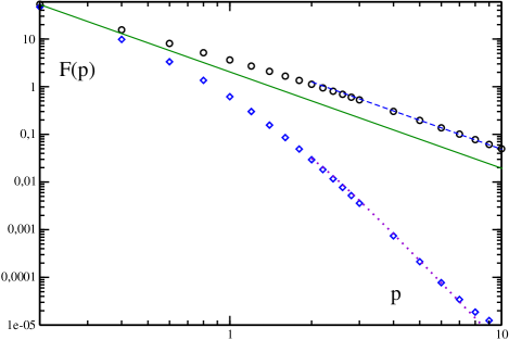
Figure 1: The integrand function $F(p)$ defined in Eq. (3.23): circles: the unsubtracted function; dashed line: asymptotic behaviour $a/p^{2}$; solid line: zero mode contribution $2/p^{2}$; diamonds: the subtracted function; dotted line: asymptotic behaviour $\propto 1/p^{6}$ of the subtracted function.

The zero mode poles are part of the asymptotic Green’ s function; if they were removed, the asymptotic behaviour of the subtracted Green’s function would be $-2/p^{2}$ and its integral would again be divergent. We neither have a prescription to handle this divergence nor the one of the separated zero mode pole. So within usual renormalized perturbation theory there is no obvious way to quantify the contribution of the collective string oscillations to the total one-loop fluctuation energy: the renormalization of the contribution of collective fluctuations to the string tension is embedded into the renormalization of the entire one-loop contribution within the framework of renormalized quantum field theory. It is not necessary to invoke a mathematical definition of divergent sums like the zeta function regularization.

There is further a conceptual difference between the zero point energy of the collective fluctuations in a string picture and their contribution to the one-loop corrections in quantum field theory: In a pure string picture the presence of fluctuations trivially requires the presence of the string. Once included their zero point energies are added to the string tension. So, if their contribution were be finite it would positive. In quantum field theory the fluctuations of the field are present even in the absence of the vortex. The vortex generates an attractive potential. The presence of the zero modes implies that levels of a continuum which starts at energies larger than $m_{W}$ or $m_{H}$ are pulled down such that at least in one channel the continuum starts at energy zero. So we expect a negative contribution to the string tension. Indeed the unsubtracted function $F(p)$ is positive and if the integral of Eq. (3.24) were finite, $\sigma_{\rm fl}$ would be negative. This simple feature gets obscured in the process of regularization and renormalization.

6 Conclusions

We have considered here a particular aspect of the one-loop corrections to the string tension of the Nielsen-Olesen vortex, the rôle of the translation modes. We have identified their wave functions and derived their contribution to the string tension. This contribution describes the energy of transversal waves propagating along the direction of the string. These can be considered as collective fluctuations of the classical vortex, in the same way as the translation modes of quantum kinks describe the collective motion of the kink. This relation is made precise, in both cases, by virial theorems. The effective action for the fluctuations is found to be the nonrelativistic limit of the Nambu-Goto action.

For the handling of the divergent one-loop corrections we have discussed conceptual differences between standard string theory and the vortex of the Abelian Higgs model. In the latter case the divergences associated with the the zero point energies of collective fluctuations are treated along with those of other fluctuations within the standard framework of renormalized quantum field theory.

The approach described here only pertains to a straight line vortex of infinite length. It can be expected to hold for more general string configurations as long as the curvature radii and a possible finite length are large compared with the transverse extension of the string. The conceptual differences in renormalization between the idealized string model and the vortex of a quantum field theory are of course of an entirely general nature. Indeed they are more general than the special model considered here. E.g., if we elevate a kink of an $1+1$ dimensional quantum field theory to a domain wall in $3+1$ dimensions, its translation mode reappears in the form of collective surface oscillations and the renormalization of this degree of freedom is again embedded into the renormalization of the energy of all quantum fluctuations.

Appendix A The translation mode

The fluctuation operator for the coupled system of transverse gauge and Higgs fields was derived in Ref. [8] in a basis of partial waves with “magnetic” quantum numbers $m$, proportional to $\exp(im\varphi)$. We refer to this reference for details. Essentially, the amplitudes $F_{4}^{m}$ corresponds to the real part of the Higgs field $\varphi_{1}$, $F_{3}^{m}$ to the imaginary part of the Higgs field $\varphi_{2}$, and the amplitudes $F_{1}^{m}$ and $F_{2}^{m}$ to combinations of the transverse gauge fields $a_{1},a_{2}$. The basis was chosen in such a way that the fluctuation operator becomes symmetric, and the amplitudes are real relative to each other. The amplitudes $F_{i}$ for $m=1$ satisfy the following coupled system of linear differential equations:

$$\left\{-\frac{1}{r}\frac{d}{dr}r\frac{d}{dr}+m_{W}^{2}f^{2}\right\}F^{1}_{1}+\sqrt{2}m_{W}f^{\prime}F^{1}_{3}+\sqrt{2}m_{W}\frac{A+1}{r}fF^{1}_{4}=0$$ (A.1)

$$\left\{-\frac{1}{r}\frac{d}{dr}r\frac{d}{dr}+\frac{4}{r^{2}}+m_{W}^{2}f^{2}\right\}F^{1}_{2}+\sqrt{2}m_{W}f^{\prime}F^{1}_{3}-\sqrt{2}m_{W}\frac{A+1}{r}fF^{1}_{4}=0$$ (A.2)

$$\left\{-\frac{1}{r}\frac{d}{dr}r\frac{d}{dr}+\frac{1}{r^{2}}+\frac{(A+1)^{2}}{r^{2}}+m_{W}^{2}f^{2}+\frac{m_{H}^{2}}{2}\left(f^{2}-1\right)\right\}F^{1}_{3}$$

$$+\sqrt{2}m_{W}f^{\prime}(F^{1}_{1}+F_{2})-2\frac{A+1}{r}F^{1}_{4}=0$$ (A.3)

$$\left\{-\frac{1}{r}\frac{d}{dr}r\frac{d}{dr}+\frac{1}{r^{2}}+\frac{(A+1)^{2}}{r^{2}}+\frac{m_{H}^{2}}{2}\left(3f^{2}-1\right)\right\}F^{1}_{4}$$

$$+\sqrt{2}m_{W}\frac{A+1}{r}(F^{1}_{1}-F^{1}_{2})-2\frac{A+1}{r}F^{1}_{3}=0 \;.$$ (A.4)

The last equation corresponds to the real part of the fluctuations of the field $\phi$, and the translation mode is obtained as $\nabla\phi_{cl}=\hat{x}vf^{\prime}$. We therefore start with the ansatz

$$F^{1}_{4}=cf^{\prime}\;,$$ (A.5)

where the coefficient $c$ is a prefactor that will be fixed later. Applying the derivative $d/dr$ to the equation of motion for $F_{4}^{1}$ we find

$$\frac{d}{dr}\left\{-\frac{1}{r}\frac{d}{dr}r\frac{d}{dr}+\frac{\left[A(r)+1\right]^{2}}{r^{2}}+\frac{m^{2}_{H}}{2}\left[f^{2}(r)-1\right]\right\}f(r) =$$

$$\left\{-\frac{1}{r}\frac{d}{dr}r\frac{d}{dr}+\frac{\left[A(r)+1\right]^{2}}{r^{2}}+\frac{m^{2}_{H}}{2}\left[3f^{2}(r)-1\right]\right\}f^{\prime}$$

$$-2\frac{(A+1)^{2}}{r^{3}}f+2\frac{A+1}{r^{2}}fA^{\prime} = 0\;.$$ (A.6)

This is the equation of motion for $F_{1}$ if the choose

$$F_{3}^{1}=c\frac{A+1}{r}f$$ (A.7)

$$F_{1}^{1}-F_{2}^{1}=c\frac{\sqrt{2}}{m_{W}}\frac{A^{\prime}}{r}\;.$$ (A.8)

The assignment has to be checked for consistency with the remaining equations of motion. Multiplying the equation of motion of $f(r)$ with $(A+1)/r$ and commuting this factor with the derivatives we find

$$\frac{A+1}{r}\left\{-\frac{1}{r}\frac{d}{dr}r\frac{d}{dr}+\frac{\left[A(r)+1\right]^{2}}{r^{2}}+\frac{m^{2}_{H}}{2}\left[f^{2}(r)-1\right]\right\}f(r) =$$

$$\left\{-\frac{1}{r}\frac{d}{dr}r\frac{d}{dr}+\frac{1}{r^{2}}+\frac{\left[A(r)+1\right]^{2}}{r^{2}}+\frac{m^{2}_{H}}{2}\left[f^{2}(r)-1\right]+m_{W}^{2}f^{2}\right\}\frac{A+1}{r}f(r)$$

$$-2\frac{(A+1)^{2}}{r^{2}}f^{\prime}+2f^{\prime}\frac{A^{\prime}}{r}=0 \;.$$ (A.9)

In the intermediate steps we have used the equation of motion for $A(r)$ in order to replace a second derivative $A"$. The result is consistent with the previous assignement if we choose

$$F_{1}^{1}+F_{2}^{2}=c\frac{\sqrt{2}}{m_{W}}\frac{A^{\prime}}{r}\;.$$ (A.10)

So we find

$$F_{2}^{1} = 0$$ (A.11)

$$F_{1}^{1} = c\frac{\sqrt{2}}{m_{W}}\frac{A^{\prime}}{r}\;.$$ (A.12)

This has to be verified by deriving the equation of motion for $A^{\prime}/r$. We obtain it by applying $1/r~{}d/dr$ to the classical equation of motion for $A(r)$:

$$\frac{1}{r}\frac{d}{dr}\left\{-r\frac{d}{dr}\frac{1}{r}\frac{d}{dr}+m^{2}_{W}f^{2}\right\}\left[A+1\right] =$$

$$\left\{-\frac{1}{r}\frac{d}{dr}r\frac{d}{dr}+m_{W}^{2}f^{2}\right\}\frac{A^{\prime}}{r}+2m_{W}^{2}\frac{A+1}{r}ff^{\prime}=0 \;.$$ (A.13)

This is consistent with the previous assigments and the equation of motion for $F_{1}^{1}$.

So we have derived that the wave function of the translation mode with $m=1$ is given by

$$\left(\begin{array}[]{c}F_{1}^{1}\\ F_{2}^{1}\\ F_{3}^{1}\\ F_{4}^{1}\end{array}\right)=c\left(\begin{array}[]{c}\sqrt{2}/m_{W}~{}A^{\prime}/r\\ 0\\ (A+1)f/r\\ f^{\prime}\end{array}\right)$$ (A.14)

We have started this derivation by considering the gradient applied to the scalar field $\phi=vf(r)$, but this has fixed only the component $F_{4}$. The component $F_{3}$ is easily seen as arising from replacing the derivatives $\nabla_{i}$ by the covariant derivatives $\nabla_{i}-igA_{i}$. The wave function for the vector potential is not given by an infinitesimal shift of the classical potential, but it correctly describes the shift in the classical magnetic field.

There is of course a second translation mode, with $m=-1$. Its wave function is given by

$$\left(\begin{array}[]{c}F_{1}^{-1}\\ F_{2}^{-1}\\ F_{3}^{-1}\\ F_{4}^{-1}\end{array}\right)=c^{\prime}\left(\begin{array}[]{c}0\\ \sqrt{2}/m_{W}~{}A^{\prime}/r\\ -(A+1)f/r\\ f^{\prime}\end{array}\right)$$ (A.15)

From these wave functions in the azimutal basis and in terms of the amplitudes $F_{i}^{\pm 1}$ we go back to the physical basis $\varphi_{1},\varphi_{2},a_{1},a_{2}$. These are related to the functions $F_{i}^{1}$ via

$$\left(\begin{array}[]{c}a_{1}\\ a_{2}\\ \varphi_{1}\\ \varphi_{2}\end{array}\right)=\frac{1}{\sqrt{2\pi}}\left(\begin{array}[]{c}(F_{1}^{1}+F_{1}^{1*})/\sqrt{2}\\ i(F_{1}^{1}-F_{1}^{1*}/\sqrt{2}\\ -i[F_{4}^{1}\exp(i\varphi)-F_{4}^{1*}\exp(-i\varphi)]\\ F_{3}^{1}\exp(i\varphi)+F_{3}^{1*}\exp(-i\varphi)\end{array}\right)$$ (A.16)

Here we have used reality constraints for the fields in order to eliminate the functions $F_{i}^{-1}$. The wave functions corresponding to infinitesimal translations into the $x$ and $y$ directions are obtained by choosing the free coefficient $c$ is such a way that the real part of the Higgs field fluctuation $\varphi_{1}$ is given by $d\phi_{\rm cl}/dx$ and $d\phi_{\rm cl}/dy$, respectively. Explicitly, $c_{x}=iv\sqrt{\pi/2}$ and $c_{y}=v\sqrt{\pi/2}$. The complete wave functions are given in section 4.

Appendix B The virial theorem

As we have discussed in section 4 the normalization of the translation mode derived from the deformation of the classical solution is given by

$$|\psi_{t}|^{2}=\pi v^{2}\int r~{}dr~{}\left\{\frac{2}{m_{W}^{2}}\frac{A^{\prime}{}^{2}(r)}{r^{2}}+\frac{(A(r)+1)^{2}}{r^{2}}f^{2}(r)+f^{\prime}{}^{2}(r)\right\}$$ (B.1)

The classical string tension is given by Eq. (2.6), i.e.,

$$\sigma_{\rm cl} = \pi v^{2}\int r~{}dr~{}\left\{\frac{1}{m_{W}^{2}}\frac{A^{\prime}{}^{2}(r)}{r^{2}}+\frac{(A(r)+1)^{2}}{r^{2}}f^{2}(r)+f^{\prime}{}^{2}(r)\right.$$ (B.2)

$$\left.\hskip 71.13188pt+\frac{m_{H}^{2}}{4}\left[f^{2}(r)-1\right]^{2}\right\}$$

In analogy with the virial theorem for quantum kinks, where the normalization of the translation mode is equal to the classical mass, we expect a virial theorem $|\psi_{t}|^{2}=\sigma_{\rm cl}$ which reduces to the identity

$$\int r~{}dr~{}\frac{1}{m_{W}^{2}}\frac{A^{\prime}{}^{2}(r)}{r^{2}}=\int r~{}dr~{}\frac{m_{H}^{2}}{4}\left(f^{2}(r)-1\right)^{2}\;.$$ (B.3)

It can readily be verified numerically. In order to derive the relation analytically we use the following weighted integrals over the classical equations of motion

$$I_{1}=\int r~{}dr~{}f\left\{-\frac{1}{r}\frac{d}{dr}r\frac{d}{dr}+\frac{\left[A+1\right]^{2}}{r^{2}}+\frac{m^{2}_{H}}{2}\left(f^{2}-1\right)\right\}f=0$$ (B.4)

$$I_{2}=\int r~{}dr~{}fr\frac{d}{dr}\left\{-\frac{1}{r}\frac{d}{dr}r\frac{d}{dr}+\frac{\left[A+1\right]^{2}}{r^{2}}+\frac{m^{2}_{H}}{2}\left(f^{2}-1\right)\right\}f=0$$ (B.5)

$$I_{3}=\int dr~{}(A+1)\frac{d}{dr}\left\{-r\frac{d}{dr}\frac{1}{r}\frac{d}{dr}+m^{2}_{W}f^{2}\right\}\left(A+1\right)=0\hskip 71.13188pt$$ (B.6)

Integrating by parts these take the form

$$I_{1} = \int r~{}dr~{}\left\{\left(\frac{df}{dr}\right)^{2}+\frac{(A+1)^{2}}{r^{2}}f^{2}+\frac{m_{H}^{2}}{2}f^{2}(f^{2}-1)\right\}=0$$ (B.7)

$$I_{2} = \int r~{}dr~{}\left\{-2\left(\frac{df}{dr}\right)^{2}-2\frac{(A+1)^{2}}{r^{2}}f^{2}-m_{H}^{2}f^{2}(f^{2}-1)\right.$$ (B.8)

$$\left.\hskip 71.13188pt+\frac{m_{H}^{2}}{4}(f^{2}-1)^{2}-\frac{(A+1)^{2}}{r}ff^{\prime}\right\}=0$$

$$I_{3} = \int r~{}dr~{}\left\{-\frac{A^{\prime}{}^{2}}{r^{2}}+m_{W}^{2}\frac{(A+1)^{2}}{r}ff^{\prime}\right\}$$ (B.9)

Combining the first and second integral we find

$$I_{2}+2I_{1}=\int r~{}dr~{}\left\{\frac{m_{H}^{2}}{4}(f^{2}-1)^{2}-\frac{(A+1)^{2}}{r}ff^{\prime}\right\}=0$$ (B.10)

Adding the third integral we obtain the relation

$$I_{2}+2I_{1}+\frac{1}{m_{W}^{2}}I_{3}=\int r~{}dr~{}\left\{-\frac{1}{m_{W}^{2}}\frac{A^{\prime}{}^{2}}{r^{2}}+\frac{m_{H}^{2}}{4}\left(f^{2}-1\right)^{2}\right\}=0$$ (B.11)

which is the expected result.

References

[1]
H. B. Nielsen and P. Olesen,
Nucl. Phys. B61, 45 (1973).
[2]
M. B. Green, J. H. Schwarz and E. Witten,
Cambridge, Uk: Univ. Pr. ( 1987) 469 P. ( Cambridge Monographs On
Mathematical Physics).
[3]
R. Rajaraman,
Amsterdam, Netherlands: North-holland ( 1982) 409p.
[4]
S. Coleman,
Aspects of Symmetry (Cambridge University Press, 1985).
[5]
J. Kripfganz and A. Ringwald,
Mod. Phys. Lett. A5, 675 (1990).
[6]
J. Baacke and T. Daiber,
Phys. Rev. D51, 795 (1995), [hep-th/9408010].
[7]
J. Baacke,
Phys. Rev. D78, 065039 (2008), [0803.4333].
[8]
J. Baacke and N. Kevlishvili,
Phys. Rev. D78, 085008 (2008), [0806.4349].
[9]
A. A. Abrikosov,
Sov. Phys. JETP 32, 1442 (1957).
[10]
H. J. de Vega and F. A. Schaposnik,
Phys. Rev. D14, 1100 (1976).
[11]
J. Baacke and G. Krusemann,
Z. Phys. C30, 413 (1986).
[12]
N. Graham, R. L. Jaffe and H. Weigel,
Int. J. Mod. Phys. A17, 846 (2002), [hep-th/0201148].