Buckled circular monolayer graphene: a graphene nano-bowl

Abstract

We investigate the stability of circular monolayer graphene subjected to a radial load using non-equilibrium molecular dynamics simulations. When monolayer graphene is radially stressed, after some small circular strain ($\sim 0.4\%$) it buckles and bends into a new bowl like shape. Young’s modulus is calculated from the linear relation between stress and strain before the buckling threshold, which is in agreement with experimental results. The prediction of elasticity theory for the buckling threshold of a radially stressed plate is presented and its results are compared to the one of our atomistic simulation. Jarzynski equality is used to estimate the difference between the free energy of the non-compressed states and the buckled states. From a calculation of the free energy we obtain the optimum radius for which the system feels the minimum boundary stress.

PACS: 62.25.-g, 46.70.Hg, 62.20.D-

1 Introduction

Graphene, is a newly discovered almost flat one-atom-thick layer of carbon atoms which exhibits unique electronic properties and unusual mechanical properties [1, 2]. At non-zero temperature graphene is not a perfect flat sheet. Recent experimental observations have found ripples in suspended sheets of graphene [3]. Atomistic simulations of graphene suggest that the strong bonds between carbon atoms in graphene is responsible for the ripples [4]. Controlling the creation of one and two-dimensional periodic ripples is possible in suspended graphene sheets by using both externally and thermally generated strains [5].

Tensional strain in monolayer graphene affects the electronic structure of graphene. For example strains larger than $15\%$ changes graphene’s band structure and leads to the opening of an electronic gap [6]. The strain can generate a bulk spectral gap in the absence of electron-electron interaction as was found within linear elasticity theory in combination with a tight-binding approach [7]. In recent experiments the buckling strain of a graphene sheet that was positioned on top of a substrate was found to be six orders of magnitude larger (i.e. $0.5-0.6\%$) than for graphene suspended in air [8]. Furthermore, some experiments showed that compressed rectangular monolayer graphene on a plastic beam with size 30$\times$100 $\mu m^{2}$ is buckled at about 0.7$\%$ strain [9]. These experiments indicate that in spite of the infinitely small thickness of the monolayer of graphene, supporting graphene by various substrates enhances the buckling strain considerably beyond the very small values ($\sim 10^{-6}\%$) obtained from elasticity theory (for very thin plate) using classical Euler analysis [8]. Although elasticity theory predicts that the very small thickness of graphene yields a zero flexural rigidity but the bond-angle effects on the C-C interatomic interaction (three body terms in Brenner’s potential) gives a non zero flexural rigidity for graphene [10]. Furthermore, elasticity theory indicates that the dimensionless critical load (buckling load) parameter depends on the thickness, radius and mechanical properties of the circular plate. It is found that it decreases nonlinearly with the thickness-radius ratio and approaches a constant value for very small thickness-radius ratios, i.e. the Kirchhoff buckling load factor, independent of the boundary conditions [11, 12, 13, 14].

Using computer simulations it is possible to calculate various thermomechanical properties of new nano scale objects and to propose new nano-structures [15]. Graphene as a nano balloon [16] is such an example where, first-principles density functional theory was used to investigate the penetration of helium atoms through a graphene monolayer with defects [17]. Density functional theory has been employed to investigate the structural, electronic and mechanical properties of rectangular graphene nanoribbons subjected to boundary stress [18] and central load [19]. Larger values for the 2-dimensional Young’s modulus with respect to the one for bulk graphene  [19] were predicted and a decreasing 2-dimensional Young’s modulus with respect to the size was reported for small size ($\sim$ 1-5 nm) of graphene nanoribbons [18]. Recently, we studied the possible deformations of rectangular graphene nano-ribbons (GNRs) at room temperature under axial strain for both free and laterally supported boundary conditions [20]. We found several longitudinal sinusoidal deformation modes for different sizes of GNRs and investigated the thermal stability of buckled GNRs. In such a study the calculation of the free energy difference is important in order to compare the stability of various structural states of stressed graphene. Thermodynamic integration and the perturbation method are two time consuming methods that have been used to calculate the difference in free energy [21]. But a more approporiate approach is based on the Jarzynski [22] identity that is valid for non-equilibrium simulations and is applicable to the study of the stability of compressed and stretched graphene.

Here, we study the mechanical stiffness of circular monolayer graphene (CMG) by investigating its linear response to strain. Using the stress-strain curve in the linear regime, we obtain Young’s modulus and the pre-stress in the CMGs which we found to be in good agreement with previous experimental and theoretical studies. Our simulations introduce a way to calculate pre-stresses which, to the best of our knowledge, is the first time that they have been calculated. After continuing the compression, CMG starts to buckle. The buckling strain in most cases are larger than the predictions from elasticity theory. Moreover the stability of a new state of radial compressed CMG which we call nano-bowl graphene (NBG), and the optimum size of CMG are studied by using atomistic simulations and the Jarzynski identity for the calculation of the free energy [22]. To the best of our knowledge this is the first time that such a free energy calculation approach is used in the field of thermomechanical properties of graphene. Recently, Colonna et al used the free energy integration based method to explain the melting properties of graphite  [23]. Our nano-scale bowl like structure for CMG is a buckled state of the thinnest material in the world.

This paper is organized as follows. In Sec. 2 we introduce the atomistic model, the simulation method and a discussion on the Jarzynski’s equality as a method to estimate the free energy difference between two states within a non-equilibrium simulation. In Sec. 3 we present our numerical results. Estimation of the Young’s modulus and pre-stresses, estimation of the buckling thresholds, the free energy changes during compression of the CMG and the stability of the obtained bowl like shape of the compressed CMG are the main results of this study. After giving our results for buckling, we present the prediction from elasticity theory for the buckling of a circular plate and compare them to the one obtained from molecular dynamics simulation. Also a discussion on the effect of the thickness of graphene on its mechanical properties is presented. In Sec. 4 we conclude the paper.

2 Method and model

Classical atomistic molecular dynamics simulation (MD) is employed to simulate compressed suspended CMG using Brenner’s bond-order potential [24]. A rigidly clamped boundary condition was imposed on a CMG with inner initial radius $a$. The boundary atoms were located in the radial distances $[a,a+2~{}\AA]$. In Fig. 1 we depict a schematic model for both side view and top view of a CMG under radial stress with clamped boundary condition and list all relevant variables describing CMG under radial stress. We simulated the system at room temperature and 50 K by employing a Nos’e-Hoover thermostat. Total number of atoms inside the boundary varies from 2224 to 18148 and there are 300 to 850 atoms at the boundaries. Initially the coordinates of all atoms are put in a flat surface of a honey comb lattice with nearest neighbor distance equal to 1.42 Å  and the initial velocities in each direction were extracted from a Maxwell-Boltzman distribution for the given temperature.

First we equilibrated the system during a time $t_{0}$ (process ‘S’), then we started to compress the system in the radial direction (process ‘I’) with the rate of compression $\mu$=0.48 m/s. The radius ($R$) at time $t$ during the process ‘I’ and the absolute value of the boundary strain are

$$R=a-\mu(t-t_{0})~{};~{}\epsilon=\frac{\mu(t-t_{0})}{a}.$$ (1)

When compressing the system, the radius of the system is reduced by very small steps (0.012 Å) to achieve a quasi-stable situation. After each compression step, we wait 2.5 ps to allow the system to relax. Note that the initial radius $a$ is for a perfect flat sheet which is not necessarily the equilibrium radius of the system (i.e. optimum size; $R_{M}$) as we will find later. At the end of process ‘I’ we relaxed the system to the new obtained radius $R_{comp}=a-\delta$ where $\delta=\mu(t_{1}-t_{0})$, (process ‘II’). For example for $a=10$ nm, setting $t_{1}$=500 ps with $t_{0}$=250 ps gives a small radial strain $\epsilon=$1.2$\%$

An important theoretical property is the free energy which is a global property which depends on the extent of the configuration space accessible to the system. In general this phase space is huge , but in practice it is sufficient to obtain an estimate of only the difference of the free energy between two related states of the system. This difference corresponds to the relative probability of finding the system in one state as opposed to the other. Thermodynamic integration and perturbation method are two common approaches to calculate this difference in the free energy [23]. In traditional methods (for example in the perturbation method) only when two states are close in their phase-space coverage, the convergence of the algorithm is good [21]. A robust and more general approach, which is also valid for non-equilibrium thermodynamics, is based on the Jarzynski equality [22] whose only requirement is a slow (quasi static) transformation between the two states (which not necessarily have to be close in phase space).

Due to the application of external forces on the boundary of the CMGs, an equilibrium approach is no longer applicable and non-equilibrium molecular dynamics simulation is needed. In the present paper we are interested to find the change in the difference between the free energy of two states: the initial non-compressed graphene membrane and a new found state of compressed CMG which we call nano-bowl graphene (NBG). In the ideal case with infinitely small or quasi-static transformation of the parameters of the system, the system will evolve along a path starting from state ‘A’ to state ‘B’. In such a case the total work done on the system is equal to the difference between the Helmholtz free energy of the two states independent of the used path (i.e. second law of thermodynamics). By contrast when the system evolves with a finite rate, as in common molecular dynamics simulations, the total work depends on the microscopic initial conditions and the above mentioned equality fails, i.e, $\Delta F=F_{B}-F_{A}\neq W$.

Independent of the path and the evolution rate between two thermodynamical states, Jarzynski found the following equality between the difference of the free energy and the total work done on the system [22]

$$\Delta F=-\beta^{-1}\ln\langle{\exp(-\beta W)}\rangle,$$ (2)

where $\beta=1/k_{B}T$. The averaging is done over the possible realizations of the switching process between the initial and the final state. Notice that Eq. (2) connects the difference of the equilibrium free energy between states ‘A’ and ‘B’ and the non-equilibrium work done when going from ‘A’ to ‘B’ even in the presence of a thermostat [22, 25].

For sufficiently slow switching between the states ‘A’ and ‘B’ the obtained values for $W$ are distributed Gaussian and only the two first terms of the expansion according to Eq. (2) will survive, i.e. $\Delta F=\langle W\rangle-\frac{\beta{\sigma_{w}}^{2}}{2}$, here the second term is the dissipated work as a consequence of fluctuations in $W$ [22]. When the parameters are changed with a finite rate, $W$ will depend on the microscopic initial conditions of the system and the reservoir (i.e. thermostat) and the average of $W$ becomes larger than $\Delta F$,

$$\langle W\rangle\geq\Delta F.$$ (3)

Higher evolution rates result in a larger difference $\langle W\rangle-\Delta F$ (larger $\sigma_{w}$) (for more discussion see Ref. [21]). Moreover it is important to mention that the value of $exp(-\beta W)$ in Eq. (2) should be obtained through a high precision calculation.

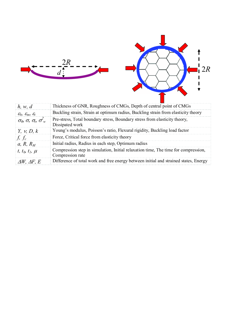
Figure 1: (Color online) Schematic model for a circular plate under radial stress with clamped boundary condition. Left picture is the side view and the right picture is the top view. We list all relevant variables describing the CMGs. Arrows show the applied boundary forces.

3 Simulation results

3.1 Young’s modulus and pre-stress

We compressed the system during process ‘I’ and calculated the total force applied on the boundary atoms at time $t$ ($t_{0}<t<t_{1}$) with radius $R$. We find the applied force on the inside boundary atoms ($f$) as the minus of the force acting on the boundary atoms. The corresponding radial boundary stress on the inside region is calculated by

$$\sigma=\frac{f}{2\pi Rh}.$$ (4)

We performed several simulations for different radius $a$ at $T$=300 K, $t_{0}$=25 ps, and the thickness of CMG $h\simeq 0.335$ nm [1]. Figure 2(a) shows the variation of the radial boundary stress (-$\sigma$) versus radial strain, i.e. stress-strain curve, for the two radii $a$=6 and 12 nm. We found that before buckling, during process ‘I’, the radial boundary stress increases linearly, and satisfies a simple linear relation between stress and strain, $\sigma=\sigma_{0}+\epsilon Y$. For small strains anharmonicity is weak [26]. By calculating the slopes of the dashed lines given in Fig. 2(a), we found the (effective) Young’s modulus ($Y$) for different radii and listed them in Table 1. The obtained Young’s modulus are in the range of recent experimental measured values, i.e. 0.5-1.01 TPa [1, 27]. Notice that the obtained Young’s modulus depends on the used value for the thickness. In the case of a single atom thick membrane (graphene), one should be careful about the definition and dimension of the Young’s modulus. Since external stress is applied on the boundary of graphene which is an almost one dimensional curve, (here the perimeter of the CMG), thus the exact unit for $Y$ should be N/m (or TPaÅ). For comparison purposes we listed $Y$s with TPa Å unit [18] in the second row of Table 1 and also showed it in the inset of Fig. 2(a). However usually by dividing this number by the thickness of graphene, $Y$ is reported in Pascal [1]. Here we used for the thickness $h$=3.35 Å as done in the experimental papers and therefore there should be no misinterpretation. In Fig. 2(a) the y-intercept, $\sigma_{0}$, is the pre-stress in the system, which occurs because our initial system with radius $a$ is not in an equilibrium state with optimum radius. The pre-stresses are 2.34 and 1.946 GPa for the two radii $a$=6, 12 nm, respectively. These pre-stresses are of the same order of magnitude as the values, e.g. 2.23 and 1.19 GPa that were measured on two flakes with diameter 1 and 1.5 $\mu m$ [1] and are also in agreement with those found in our previous study on GNRs [20]. At zero strain, the sign of the pre-stresses indicate that the inside atoms exert an inward stress on the boundary atoms. Furthermore, note that here (except for the two smallest CMGs) Young’s modulus varies (around 0.525 TPa) with respect to the size of the CMGs. Young’s modulus of graphene nano-ribbons depends on the size of the system. The chrematistic length of graphene (8-10 nm  [4]) is a measure of the range over which the deformations in one region of graphene are correlated with those in another region, so the applied boundary stresses on the edges do not affect the system beyond this characteristic length. We expect that our system with radius less than the characteristic length ($2a<$12 nm) will show a larger $Y$. But we believe that this behavior depends also on the applied boundary condition, i.e. clamped boundary condition. Faccio et al  [18] and Hod et al  [19] used density functional theory and found a larger value for $Y$ for smaller size graphene nano-ribbons (less than 6 nm) and reported a decreasing $Y$ with increasing size of nano-ribbons.

3.2 Buckling results

3.2.1 Molecular dynamics predictions for buckling of CMG

Beyond the linear regime and during process ‘I’, we estimate the critical buckling stress. The rapid increase of the lateral deflection with load near the buckling threshold defines experimentally the buckling stress [11]. In our simulations we estimated the buckling points as the points where the roughness of the system suddenly increases. In Fig. 2(b) we show the variation of the root mean square displacement -$w$- (rms) of the z-component of the CMG versus applied strain for two radii $a$=6 and 12 nm. The buckling point is obtained with a uncertainly which increases with decreasing size of the membrane which results in larger error bars on the buckling strain for small systems. The sudden change in the slope of these curves are directly related to the buckling threshold (solid arrows in Fig. 2(b)). For small applied strain (i.e. below the buckling points) $w$ exhibits random fluctuations which are due to the applied boundary stress and the thermal fluctuations. The inset of Fig. 2(b) shows the depth, $d$ (the z-components of the atoms in the center of CMG), of the buckled CMG versus strain which exhibits a clear nonlinear dependence. It is interesting to note that we found that for larger sizes (i.e. $a\geq 8$ nm) the buckling strain is only slightly modified. In this limit the size of CMGs are beyond the characteristic length of graphene  [4]. Usually, the mechanical properties of graphene are found to be unchanged for systems that have larger sizes than the characteristic length [28]. Therefore it is not necessary to simulate systems with larger radii.

The boundary strains ($\epsilon_{b}$) are listed in Table 1. The obtained values show a non-linear decrease with increasing radius as shown by solid dots in Fig. 2(c). Larger buckling strains are found for smaller systems. This behavior is confirmed by recent quantum molecular dynamics simulation [29], where for a small system with size 1.99$\times$0.738 $nm^{2}$ a buckling strain of 0.8$\%$ was found.

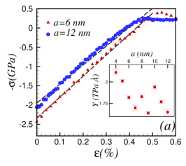
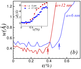
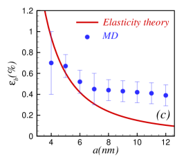
Figure 2: (Color online) (a) Variation of the radial in-plane stress (radially inward direction) applied on the boundary versus the radial boundary strain for two different radii of circular monolayer graphene, i.e. 6 and 12 nm. The dashed lines are fitted to the numerical results in the region before the buckling threshold. The inset shows the Young’s modulus as a function of the radius. (b) Variation of the root mean square displacement of the z-component of atoms of CMGs versus the applied boundary strain for two radii $a$=6 and 12 nm. The inset shows the variation of the depth of the buckled circular monolayer graphene versus strain. (c) Circular dots are from our numerical simulations for the buckling strain and the solid line is the prediction from elasticity theory when the thickness of graphene was set to 0.335 nm.

$a~{}(nm)$	4.0	5.0	6.0	7.0	8.0
$Y$(TPa)	0.631$\pm$8.0	0.601$\pm$6.0	0.543$\pm$7.0	0.507$\pm$8.0	0.546$\pm$8.0
$Y$(TPa Å)	2.11$\pm$0.03	2.01$\pm$0.02	1.82$\pm$0.02	1.70$\pm$0.03	1.83$\pm$0.03
$\epsilon_{b}(\%)$	0.71$\pm$0.3	0.67$\pm$0.1	0.52$\pm$0.1	0.45$\pm$0.2	0.44$\pm$0.1
$a~{}(nm)$	9.0	10.0	11.0	12.0
$Y$(TPa)	0.490$\pm$9.0	0.579$\pm$8.0	$0.528\pm$8.0	$0.492\pm$9.0
$Y$(TPa Å)	1.64$\pm$0.03	1.94$\pm$0.02	$1.77\pm$0.02	$1.65\pm$0.03
$\epsilon_{b}(\%)$	0.43$\pm$0.1	0.42$\pm$0.1	0.41$\pm$0.1	0.39$\pm$0.1

Table 1: Young’s modulus and the buckling strain for different radius of the circular monolayer graphene.

3.2.2 Elasticity theory predictions for a buckled circular plate

We will compare our results with predictions of elasticity theory for the buckling of a circular plate. The sudden structural deformation of a continuum membrane subjected to high compressive stress is called buckling. At the point of failure the actual compressive stress is less than the ultimate compressive stresses that the material is capable of withstanding. The boundary condition and the elasticity of the plate are two important parameters in determining the buckling critical load. The buckling occurs when the disturbing moment of a material equals the restoring moment [11]. The governing equation for a simple bar with length $L$ can easily be obtained by considering the curvature, bending moment and disturbing moment of the bar, i.e. Euler’s column theory [11], resulting $\frac{\pi^{2}P}{L^{2}}$ for the buckling load, where $P$ is a parameter which is related to Young’s modulus ($Y$) and the moment of inertia of the rod cross-sectional axis that is perpendicular to the buckling plane. For the case of circular plate under radial compressive force, according to continuum elasticity theory one can define the strain energy as the restoring energy in the plate due to the external forces. The minimization of the strain energy of a circular plate based on Trefftz’s theory for the linear and nonlinear components of the strain and the stress tensors results into two coupled differential equations [13, 14]. Traditionally it is better to define a dimensionless quantity -critical or buckling load factor, $k$ as $k=\frac{f_{c}a^{2}}{D}$. Here $f_{c}$ is the critical radial compressive force on the boundary per length, $D=Yh^{3}/(12(1-\nu^{2}))$ is the flexural rigidity of the plate with thickness $h$, $\nu$ is the Poisson’s ratio and $Y$ is the Young’s modulus. Flexural rigidity of a plate is defined as the force required to bend a rigid structure to a unit curvature. Poisson’s ratio is the ratio of transverse contraction strain to longitudinal extension strain in the direction of stretching force. In the case of axisymmetric buckling and the assumption of no variation in the thickness, the solution of the equations yields the Kirchhoff buckling load factor, $k_{0}(\simeq 14.6820)$, for different combinations of boundary conditions. Different boundary condition for the circular plate gives different buckling loads [13] while the atomistic structure of the plate is not included directly in the theory. For the clamped boundary condition, where the perimeter of the circular plate is not allowed for any movement, and in the absence of any pre-buckling deformation (in the system), the equation for $k$ leads to  $k=k_{0}/(1+\frac{(h/a)^{2}k_{0}}{5(1-\nu)})$ [13, 14]. Note that elasticity theory predicts that when the thickness-radius ratio is set to zero we find $k=k_{0}$ and consequently the buckling load is $\frac{k_{0}D}{a^{2}}$ which is similar to the formula for the buckling load of a bar, i.e. $\frac{\pi^{2}P}{L^{2}}$. The radial compressive force for a plate with radius $a$ can be written as

$$f_{c}=\frac{k_{0}D}{a^{2}+\frac{h^{2}k_{0}}{5(1-\nu)}}.$$ (5)

Dividing $f_{c}$ by the thickness yields the relationship between stress and strain as

$$\sigma_{t}=\frac{k_{0}h^{2}}{12(1-\nu^{2})(a^{2}+\frac{h^{2}k_{0}}{5(1-\nu)})}Y=\epsilon_{t}Y,$$ (6)

where $\epsilon_{t}$ is the theoretical buckling strain. Note that, elasticity theory predicts an inverse square dependence on the radius: $\epsilon_{t}\cong\frac{k_{0}}{12(1-\nu^{2})}\frac{h^{2}}{a^{2}}$ which is shown by the solid line in Fig. 2(c) (where $h\simeq 3.35$ Å and $\nu=0.3$ is the typical Poisson’s ratio [26]). According to elasticity theory, below the solid line the system is in the non-buckled (rippled) state and above this line it is buckled [30]. A rippled state can be understood as any thermodynamical state of graphene before buckling and under non zero boundary stress. Our results (except for $a$=4 nm) are above the thresholds found from elasticity theory. The reason is that the considerable and non-zero flexural rigidity of graphene, which is a consequence of strong $sp^{2}$ bonds [10], is responsible for those larger buckling thresholds as compared to those found from linear elasticity theory.

Note that both theoretical and MD results are sensitive to the used thickness of monolayer graphene. Larger thickness leads to a larger difference between MD results and elasticity theory. For example, by using a smaller thickness which is closer to the interatomic distance in graphene .i.e. $\simeq 0.1$ nm, predictions from elasticity theory are reduced by one order of magnitude. Recently, for the buckling experiments of embedded graphene the same disagreement was reported [8]. In fact, the thickness of graphene is an important parameter which causes several new unusual mechanical properties of graphene, particularly large stiffness with respect to other materials (physically the interpretation of the stiffness and the rigidity of single layer graphene strongly depends on the very thin thickness of graphene). This issue is important also for studying mechanical stiffness of other carbon allotropes and leads to different values for Young’s modulus etc. Please note that the thickness of graphene depends on the used interatomic potential, loading method etc [31]. We followed the approach used by experimentalists and used $h\simeq 0.335$ nm which is the interlayer spacing of graphite [1].

In order to induce significant changes in graphene’s band structure one needs even larger strains ($>15\%$) than the one we obtained from the buckling threshold [6]. Thus, in the case of compressive strain, the shape of the buckled CMGs will change appreciably before the electronic band structure is modified.

3.3 Free energy

3.3.1 Free energy change during compression of CMG

Here we will focus on the system with $a=10$ nm. Since a study of the stability of graphene needs longer simulation time, we first relaxed the system during $t_{0}$=250 ps (process ‘S’), and then compressed the system during $t_{1}$=500 ps (with the compression rate $\mu=$0.48 m/s, the applied strain rate is 0.0048/ps). At the end of process ‘I’ we relaxed the system to the new obtained radius $R_{comp}=a-\delta$ where $\delta=\mu(t_{1}-t_{0})$, i.e., process ‘II’. Setting $t_{1}$=500 ps gives a small radial strain $\epsilon_{r}=$1.2$\%$ and a reduction of the radius by $\delta=$1.2 Å. Here we discuss process ‘I’ and in the next section we return to process ‘II’.

Fig. 3(a) shows the variation of the total work performed on the system when changing the radius from the end of the ‘S’ state to the ‘II’ state. Dashed curves are the results obtained by performing simulations with different initial conditions. The solid curves are the average $\langle W\rangle$. We found that by using a small rate ($\mu$), 15 members of the ensemble are sufficient to realize convergence of the exponential ensemble averages in Eq. (2) (the reason is that the differences in $W$ between each trajectory are small). Almost the same $W$ curves indicate that the variance of the work distribution is small (here typically $\sigma_{w}<0.05$ eV). For a larger rate, a larger variance will be found [20].

In Fig. 3(b), by using the Jarzynski equality, we calculated the difference of the free energy between the states with radius $R$ and $a$, i.e. $F-F_{S}$ . In this curve $t$ is the compression time which is related to the strain from Eq. (1). Each symbol (at time $t$) is related to a quasi-static state during process ‘I’. Comparing $\langle W\rangle$ (Fig. 3(a)) and $F-F_{S}$ (Fig. 3(b)) shows that the difference in free energy is smaller than the total work. However the difference is small enough (very small $\sigma_{w}$ in Table 2) such that the chosen number of different simulations (i.e. 15) and the rate ($\mu$) are sufficient. The first minimum in the process ‘I’ is deeper for temperature $T$=300 K as compared to $T$=50 K and occurred before the buckling threshold. We call this minimum the ‘M’ point. The radius of the system at state ‘M’, i.e. $R_{M}$, is the optimum radius of the CMG where there is no boundary stress. Considering the difference in the free energy for the points ‘M’, one can estimate $\Delta F=F_{M}-F_{S}$. Some of the results for the difference in free energy, variance in $W$ distributions and $R_{M}$ are explicitly listed in Table 2. The free energy of point ‘S’ is higher than those of point ‘M’. This general behavior tells us that the starting states ‘S’ are not the relaxed states and as we showed in section 3.1 there is pre-stress in the system. From the optimum radius reported in Table 2, we see that the radius of the ‘M’ point for lower temperature is closer to the radius of the ‘S’ point, i.e. ${R_{M}}{(300~{}K)}<{R_{M}}{(50~{}K)}$. The reason is that the equilibrium state at lower temperature has a smaller out of plane deviation, or simply its state is closer to a flat plane. Furthermore, note that the conditions $R_{M}>R_{b}$ and $\epsilon_{M}=\frac{0.3\delta}{a}\simeq\frac{\sigma_{0}}{Y}$ are always satisfied where $R_{b}$ is the radius of the CMG at the buckling point.

Moreover, we calculated the ensemble average of the total energy per atom, containing both kinetic and potential energy. Fig. 3(c) shows the variation of the total energy per atom ($E/N$) versus time during the evolution S$\rightarrow$II. As one expects increasing the temperature decreases the absolute value of the total energy because of the increasing kinetic energy. In contrast to the free energy and the total performed work on the system, (Figs. 3(a,b)), here we have non zero energy values during processes ‘S’ and ‘II’. Since the total energy of the system increases for the evolution S$\rightarrow$M, we conclude that this evolution is an entropy dominated evolution ($\Delta F-\Delta E<0$ as we see from Table 2). In contrast to the total work done on the system, the average of the total energy (Fig. 3(c)) has an overall different behavior (particularly at the ‘M’ points) from the curves shown in Figs. 3(a,b). The increasing change (not decreasing change) in the slope of the energy curves during process ‘I’, point to the ‘M’ points. We conclude that the equilibrium relaxed size of the simulated system could not be obtained by looking only at the total energy or the potential energy and that free energy considerations are necessary.

3.3.2 Stability of the nano-bowl

After compressing, CMG reaches the process ‘II’, where the radius of the CMG is $R_{comp}$ and we arrive at the state NBG. This new state is observed after the buckling threshold. Therefore all states after the buckling threshold are in the NBG state with different depths, $d$. In Figs. 3(a,b,c) the last processes are related to this new NBG state. Note that when we do not have any compression in the system both $\Delta F$ and $W$ are zero as it is clear from the flat regions during process ‘II’ in Figs. 3 (a,b). In order to be sure about the stability of the NBG at different values of strain, we performed extra long simulations for the process ‘II’ up to nanoseconds. Figure 4 shows two final snapshots of two long time simulations during process ‘II’. In this figure $a=10$ nm and total applied strains are 1.2$\%$ and $6\%$ for Fig. 3(a) and Fig. 3(b), respectively. As we see, a larger strain results in a deeper nano-bowl. These NBGs are stable and their concave shape survives independently of the considered temperature and strains. Therefore they keep their shapes and are static. The negative (positive) value for $\Delta F$ at $T$=300 K ($T$=50 K) during the evolution S$\rightarrow$II indicates that the NBG at this temperature is more (less) stable than the starting state ‘S’. Note that gravity and other external fields have been ignored and the bowl-like shape and the hump shape occur random with the same probability, and we call both shapes NBG. This concave shape should be observable experimentally using scattering experiments.

When comparing the difference of the free energy between ‘M’ and NBG, using the values in Table 2, gives $\Delta F(M\rightarrow II)$=3.2965 eV for $T$=300 K which indicates that the real optimum equilibrium state is ‘M’. Here, in all cases we see the validity of the inequality Eq. (3). Note that the differences in the free energy per atom are very small, i.e. $\leq 10^{-4}$eV.

$T$(K)	$\langle W\rangle(S\rightarrow M)$	$F_{M}-F_{S}$	$E_{M}-E_{S}$	$R_{M}$	$\sigma_{w}$
300	-3.9514 (eV)	-3.9940(eV)	$\sim$ 23(eV)	$a-0.3\delta$	0.047(eV)
50	-0.5164(eV)	-0.5688(eV)	$\sim$ 2(eV)	$a-0.11\delta$	0.021(eV)

Table 2: Total work done on the system $\langle W\rangle$, difference of the free energy (Eq. (2)), difference of the total energy, the equilibrium radius of points ‘M’ and variance in work distribution at points ‘M’ for the system with initial radius $a=10$ nm at $T$=300 K and 50 K (see Figs. 3) for $\epsilon=1.2\%$.

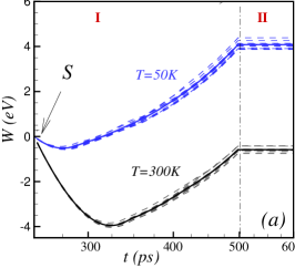
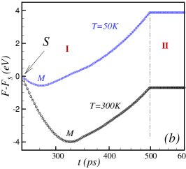
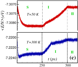
Figure 3: (Color online) (a) Total work done on the system (with initial radius a=10 nm and two different temperatures, i.e. 50 K and 300 K) during the compression of a circular monolayer graphene where the total boundary strain is $\epsilon_{r}=1.2\%$. During process ‘I’ the system is compressed for 250 ps and it reaches the radius $a$-$\delta$ at the end of this process. During the process ‘II’ we allow the system to relax in the compressed state for 250 ps. Solid curves are the average of the dashed curves. (b) Corresponding difference in the free energy (using Jarzynski equality). (c) Ensemble average of the total energy per atom of circular monolayer graphene during evolution S$\rightarrow$ II.

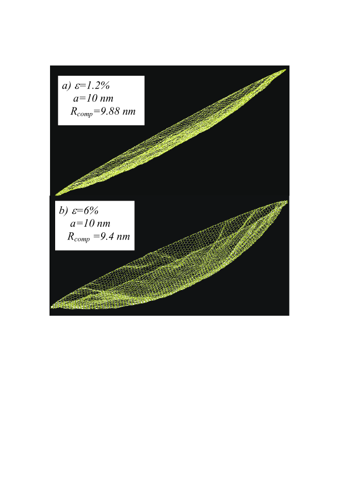
Figure 4: (Color online) Two snap shots of buckled circular monolayer graphene after applying radial boundary strains: (a) $\epsilon_{r}=1.2\%$ and (b) $\epsilon_{r}=6\%$  with initial radius $a=10$ nm at $T$=300 K.

4 Conclusions

In summary, when applying an increasing radial force on the boundary of circular monolayer graphene, first a linear response regime appears which enables us to estimate Young’s modulus and pre-stresses, which are found to be in agreement with experiments. When continuing compression, at a critical radial force, graphene starts to buckle. The computed critical buckling strains are larger than those found from elasticity theory. These states are new thermodynamically buckled stable states which we called nano-bowl. In order to investigate the thermodynamical stability of nano-bowls, we used a non-equilibrium computational method based on the Jarzynski identity. This identity enables us to calculate the difference in the free energy between the initial non-compressed state and the buckled states. Also the optimum radius of circular graphene, where there is no boundary stress, can be estimated by looking at the minimum in the free energy curve. At room temperature the nano-bowl is more stable than the initial non-compressed state which was pre-stressed. Free energy calculations based on the Jarzynski [22] equality can open a new approach to study various thermomechanical properties of compressed graphene.

5 Acknowledgment

This work was supported by the Flemish Science Foundation (FWO-Vl) and the Belgian Science Policy (IAP).

References

- [1] C. Lee, X. Wei, J. W. Kysar, and J. Hone, Science 321, 385 (2008).
- [2] T. J. Booth, P. Blake, R. R. Nair, D. Jiang, E. W. Hill, U. Bangert, A. Bleloch, M. I Gass, K. S. Novoselov, M. I. Katsnelson, and A. K. Geim, Nano. Lett. 8, 2442 (2008).
- [3] J. C. Meyer, A. K. Geim, M. I. Katsnelson, K. S. Novoselov, T. J. Booth, and S. Roth, Nature (London) 446, 60 (2007).
- [4] A. Fasolino, J. H. Los, and M. I. Katsnelson, Nature Materials 6, 858 (2007).
- [5] W. Bao, F. Miao , Z. Chen , H. Zhang , W. Jang, C. Dames, and C. Ning Lau, Nature Nanotechnology 4, 562 (2009).
- [6] F. Guinea, M. I. Katsnelson, and A. K. Geim, Nature Physics 6, 30 (2009).
- [7] V. M. Pereira, A. H. Castro Neto, and N. M. R. Peres, Phys. Rev. B 80, 045401 (2009).
- [8] O. Frank, G. Tsoukleri, J. Parthenios, K. Papagelis, I. Riaz, R. Jalil, K. S. Novoselov, and C. Galiotis, ACS-Nano 4, 3131 (2010).
- [9] G. Tsoukleri, J. Parthenios, K. Papagelis, R. Jalil, A. C. Ferrari, A. K. Geim, K. S. Novoselov, and C. Galiotis, Small 5, 2397 (2009).
- [10] M. Arroyo, T. Belytschko, Phys. Rev. B 69, 115415 (2004)
- [11] J. Singer, J. Arbocz, and T. Weller, Experimental Methods in Buckling of Thin-Walled Structures, (Wiley, 1998); R. M. Jones Buckling of Bars, Plates, and Shells (Taylor Francis, Philadelphia 1999)
- [12] A. Sakhaee-Pour, Comp. Mater. Sci. 45, 266 (2009).
- [13] G. M. Hong, C. M. Wang, and T. J. Tan, Singapore, Applied Mechanics 63, 534 (1993).
- [14] C. M. Wang, T. J. Tan, G. M. Hong, and W. A. M. Alwis, Mech. Struct. Mach. 24, 135 (1996).
- [15] B. I. Yakobson, C. J. Brabec, and J. Bernholc, Phys. Rev. Lett. 76, 2511 (1996).
- [16] J. S. Bunch, S. S. Verbridge, J. S. Alden, A. M. van der Zande, J. M. Parpia, H. G. Craighead, and P. L. McEuen, Nano. Lett. 8, 2458 (2008).
- [17] O. Leenaerts, B. Partoens, and F. M. Peeters, Appl. Phys. Lett. 93, 193107 (2008).
- [18] R. Faccio, P. A. Denis, H. Pardo, C. Goyenola, and A. lvaro WMombru, J. Phys.: Condens. Matter 21, 285304 (2009).
- [19] O. Hod and G. E. Scuseria, Nano. Lett. 9, 2619 (2009).
- [20] M. Neek-Amal and F. M. Peeters, Phys. Rev. B 82, 085432 (2010).
- [21] H. Xiong, A. Crespo, M. Marti, D. Estrin, and A. E. Roitberg, Theor. Chem. Acc. 116, 338 (2002).
- [22] C. Jarzynski, Phys. Rev. Lett. 78, 2690 (1997).
- [23] F. Colonna, J. H. Los, A. Fasolino, and E. J. Meijer, Phys. Rev. B 80, 134103 (2009).
- [24] D. W. Brenner, Phys. Rev. B 42, 9458 (1990).
- [25] M. A. Cuendet, Phys. Rev. Lett. 96, 120602 (2006).
- [26] E. Cadelano, P. L. Palla, S. Giordano, and L. Colombo, Phys. Rev. Lett. 102, 235502 (2009).
- [27] I. W. Frank, D. M. Tanenbaum, A. M. Van der Zande, and P. L. McEuen, J. Vac. Sci. Technol. B 25, 2558 (2007).
- [28] C. D. Zeinalipour-Yazdi and C. Christofides, J. Appl. Phys. 106, 054318 (2009); H. Zhao, K. Min, and N. R. Aluru, Nano. Lett. 9, 3012 (2009).
- [29] Y. Gao and P. Hao, Physca E 41, 1561 (2009).
- [30] D. P. Holmes, M. Ursiny, and A. J. Crosby, Soft Matter 4, 82 (2008).
- [31] Y. Huang, J. Wu, and K. C. Hwang, Phys. Rev. B 74, 245413 (2006).