Effect of turbulent fluctuations on the drag and lift forces on a towed sphere and its boundary layer

Abstract

The impact of turbulent fluctuations on the forces exerted by a fluid on a towed spherical particle is investigated by means of high-resolution direct numerical simulations. The measurements are carried out using a novel scheme to integrate the two-way coupling between the particle and the incompressible surrounding fluid flow maintained in a high-Reynolds-number turbulent regime. The main idea consists in combining a Fourier pseudo-spectral method for the fluid with an immersed-boundary technique to impose the no-slip boundary condition on the surface of the particle. This scheme is shown to converge as the power 3/2 of the spatial resolution. This behaviour is explained by the $L_{2}$ convergence of the Fourier representation of a velocity field displaying discontinuities of its derivative. Benchmarking of the code is performed by measuring the drag and lift coefficients and the torque-free rotation rate of a spherical particle in various configurations of an upstream-laminar carrier flow. Such studies show a good agreement with experimental and numerical measurements from other groups. A study of the turbulent wake downstream the sphere is also reported. The mean velocity deficit is shown to behave as the inverse of the distance from the particle, as predicted from classical similarity analysis. This law is reinterpreted in terms of the principle of “permanence of large eddies” that relates infrared asymptotic self-similarity to the law of decay of energy in homogeneous turbulence.

The developed method is then used to attack the problem of an upstream flow that is in a developed turbulent regime. It is shown that the average drag force increases as a function of the turbulent intensity and the particle Reynolds number. This increase is significantly larger than predicted by standard drag correlations based on laminar upstream flows. It is found that the relevant parameter is the ratio of the viscous boundary layer thickness to the dissipation scale of the ambient turbulent flow. The drag enhancement can be motivated by the modification of the mean velocity and pressure profile around the sphere by small scale turbulent fluctuations. It is demonstrated that the variance of the drag force fluctuations can be modelled by means of standard drag correlations. Temporal correlations of the drag and lift forces are also presented.

1 Introduction

The dynamics of suspended particles whose size is larger than the smallest active scales of the carrier turbulent flow is important for the understanding of many natural and industrial applications. Let us mention two concrete problems borrowed from the study of planet formation and of rain processes. In the first situation, the role of turbulence is still unsettled in the dynamical mechanisms that take place during the origination of planets in a proto-planetary disk (see, e.g., de Pater & Lissauer, 2001). A key issue is to understand whether or not the disk turbulence can generate an increase of the rate at which a large body can accrete dust. In other terms, it requires identifying the turbulent fluctuation mechanisms that lead to a snowball effect where the larger bodies have a growth speed all the more fast as their size increases. The same kind of question arises in the precipitation process when a large raindrop falls under the effect of gravity and collides with much smaller droplets that are transported by the turbulent airflow in the cloud (see Shaw, 2003). For this problem, another question is to know the efficiency of wet deposition (or scavenging) of particle pollutants that are present in the atmosphere (see, e.g., Seinfeld & Pandis, 1998). These various phenomena are still poorly understood and are subject to empirical ad-hoc modelling. Such fundamental open questions, which are taken from natural sciences but also arise in a number of industrial settings, reflect an inadequate current level of modelling for large particles in turbulent flows.

Current approaches for the dynamics of finite-size particles are commonly assuming that the particles are infinitely small (point particles) and that the Reynolds number associated to their interaction with the flow vanishes, so that their dynamics can be obtained by matching the solution to the Stokes equation in their vicinity to an unperturbed fluid velocity. Recent experimental work showed that the dynamics of finite-size particles is not well described by such models (see Qureshi et al., 2007; Xu & Bodenschatz, 2008; Volk et al., 2010). Significant size effects have been for instance measured in the acceleration statistics of such particles. Despite the fact that the flatness of the acceleration distribution depends only weakly on the diameter of the particle, its variance strongly decreases with diameter and temporal correlations of the acceleration vary with the particle size in a manner that cannot be predicted by standard point-particle models. Improved models accounting for the so-called “Faxén corrections” (spatial averages of fluid velocities and accelerations over the volume of the particle) are in much better agreement with such qualitative trends but hardly reproduce quantitatively the mentioned experimental data (see Calzavarini et al., 2009, 2011).

A key ingredient of the finite-size models mentioned above are drag correlations, which determine the forces on a sphere based on its velocity difference with the fluid. All those drag correlations are empirical formulas fitting experimental and numerical measurements of the drag experienced by a sphere in a laminar upstream flow. However, the question whether or not turbulent fluctuations eventually present in the carrier flow modify those drag correlations is an open issue, which has been under discussion for more than forty years. Several groups claim that turbulence increases the drag on a sphere (see Anderson & Uhlherr, 1977; Brucato et al., 1998) while others observe no significant modifications of the drag forces (see Warnica et al., 1995; Bagchi & Balachandar, 2003; Kim & Balachandar, 2012). See Balachandar & Eaton (2010) for a review. Recently, Luo et al. (2010) have shown that a particle in an oscillating flow experiences an increased drag force. It is difficult both for numerical and for experimental measurements to reliably measure an averaged force on the particle due to the statistical fluctuations introduced by the turbulence.

Another challenging requirement to improve models for the dynamics of finite-size particles in turbulent flows is to get a precise understanding on how the carrier flow is modified in the vicinity of the particle in situations where such effects occurs on scales which are comparable to the active scales of the surrounding turbulence. For instance, it is clear that much work is still needed in order to get a better handling on how the kinetic turbulent energy, the dissipation rate, as well as other standard statistical properties of turbulence, varies in the vicinity of the particle. Direct numerical simulations appear to be valuable candidates as they give a unique global and instantaneous access to such quantities. However, the numerical problem is challenging for several reasons: (i) the numerical approach has to resolve all active scales of a fully developed turbulent flow, which span several decades; (ii) at small scales the boundary layer around the particle is of great importance and has to be well resolved; (iii) if one considers a moving particle the algorithm has to follow the displacement of the particle accurately and efficiently; (iv) for a sufficient separation of the different scales involved (forcing scales, inertial range of scales, dissipative scales) the algorithm has to parallelize efficiently on massively parallel computers.

Several different strategies have been recently proposed in order to solve the incompressible Navier–Stokes equations together with no-slip boundary conditions at the surface of a spherical particle in a turbulent environment. All of them make use of a homogeneous grid covering the complete physical domain.

“Physalis”, which was developed by Prosperetti & Oguz (2001) and extended and used by Naso & Prosperetti (2010), makes use of known analytic solutions to the Stokes equation for the boundary layer in the vicinity of the particle, in order to describe the velocity at the nearest surface points of the grid. Iteratively, the analytic solution and the solution on the homogeneous grid are matched. An advantage of this strategy is that the no-slip condition is imposed in an exact manner. However, improvement are required in order to achieve very-large Reynolds number carrier flows (the value $\mbox{{Re}}_{\lambda}=20$ of the Taylor-microscale Reynolds number was chosen in Naso & Prosperetti, 2010). Another recently developed approach consists in using and matching two different grids. A spherical one encloses the particle surface and is designed to resolve the boundary layer and a second homogeneous grid covers the entire domain. This “Overset Grid” technique proposed by Burton & Eaton (2005) uses a third-order interpolation to transfer values from one grid to the other in order to couple the two solutions. This method was shown to reproduce very accurately experimental measurements of the drag coefficient at a particle Reynolds number of $\mbox{{Re}}_{\mathrm{p}}=20$. In turbulent settings, this method was used with a Reynolds number $\mbox{{Re}}_{\lambda}=32$. Finally, we note that Yeo et al. (2010) uses a force coupling method based on a low-order, finite force multipole representation for the influence of the particles in the flow. This efficient approach is limited to rather low particle Reynolds number of less than 20. Most of these approaches are at the moment limited to rather small carrier-flow Reynolds numbers. We propose here to use a method that allows one to reach much higher Reynolds numbers. It follows the approach of Goldstein et al. (1993) who used an immersed boundary approach together with a spectral solver. However, as Mohd-Yusof (1997), we combine here a spectral method with direct forcing instead of a feedback scheme à la Peskin (1977). Note that such a direct-forcing approach has recently been used by Uhlmann (2005) together with a finite-difference method.

This paper is organised as follows. In § 2 we present in details the proposed method, together with some considerations on its convergence. Then, in § 3, we report measurements in a laminar upstream flow. The drag and lift coefficients are measured in various settings and compared to other numerical and experimental works. We also focus on the wake properties and characterize the decay of turbulent fluctuations in the particle wake. In § 4 we turn to a particle in a fully-developed stationary turbulent upstream flow and study this case varying the turbulent intensity. The effect of fluid velocity fluctuations on the drag and lift forces are discussed and interpreted in terms of the modification of the particle boundary layer. Finally, in § 5, we draw some concluding remarks and suggest open questions.

2 Description of the numerical method

The idea of our approach is to combine a standard pseudo-Fourier-spectral with a penalty method. The former is well adapted to incompressible homogeneous and isotropic turbulence, has a high degree of accuracy, and has shown good performances on massively parallel supercomputers. No-slip boundary conditions are implemented by an immersed boundary and penalisation strategy. The proposed method is a modification of that used by Homann & Bec (2010) for investigating the dynamics of neutrally buoyant particles suspended in turbulent flows. The former version of the method was well-adapted to particles with a small velocity difference with the fluid but happened to show some limitations when the slip is too large. We present here a modification of this method that reduces such shortcomings.

The dynamics of an incompressible flow in which is embedded a spherical particle is given by the Navier-Stokes equations

$$\partial_{t}{\bm{u}}=\mathcal{L}(\bm{u})=-\bm{u}\cdot\nabla\bm{u}-\nabla p+\nu\nabla^{2}{\bm{u}}+\bm{f}_{e},\quad\nabla\cdot{\bm{u}}=0,\quad\mbox{for }|\bm{x}-\bm{X}_{p}(t)|>d/2$$ (1)

together with the no-slip boundary condition on the surface of the particle

$${\bm{u}}(\bm{x},t)=V_{\mathrm{p}}(t)+\bm{\omega}_{\mathrm{p}}(t)\times[\bm{x}-\bm{X}_{\mathrm{p}}(t)]\quad\mbox{for }|\bm{x}-\bm{X}_{p}(t)|=d/2.$$ (2)

$\bm{f}_{e}$ denotes here external forces that are exerted on the flow, $d$ is the particle diametre, $X_{\mathrm{p}}$, $\bm{V}_{\mathrm{p}}$, and $\bm{\omega}_{\mathrm{p}}$ are the particle position, translational velocity, and angular velocity, respectively. The particle dynamics is obtained by solving Newton’s equations where the force exerted by the fluid is obtained by integrating on the surface of the particle the contribution from pressure and viscous stress to the fluid stress tensor.

The numerical method presented here consists in integrating in a rectangular periodic domain the Navier–Stokes equation (1) by using a strongly-stable, low-storage Runge-Kutta scheme of third order that was introduced by Shu & Osher (1988). The spatial derivatives are evaluated in Fourier space and the nonlinear term is computed with a pseudo-spectral method using the standard dealiasing 2/3 rule (see, e.g., Patterson & Orszag, 1971). The pressure term is obtained by solving the Poisson equation directly in Fourier space. The viscous term is treated implicitly via an exponential factor.

2.1 The penalty force

To impose the no-slip boundary conditions (2) at the surface of the particle, we make use of an immersed boundary technique. It consists in introducing in the right-hand side of the Navier-Stokes equation (1) a penalty force $\bm{f}_{b}(\bm{x},t)$, which acts as a Lagrange multiplier associated to the constraint defined by the boundary condition (2). The full problem (1)-(2) can then be rewritten as

$$\partial_{t}{\bm{u}}=\mathcal{L}(\bm{u})+\bm{f}_{b},\quad\nabla\cdot{\bm{u}}=0,$$ (3)

that is satisfied in the whole domain. The core of such a method is to find the best strategy to estimate $\bm{f}_{b}$. In principle the penalty force should vanish outside the particle and be such that $\bm{u}$ is equal to a solid motion inside it. The Fourier representation of the velocity field with a finite number of modes implies that these two conditions cannot be satisfied in an exact manner. An idea could be to find at each time step $\bm{f}_{b}$ with a minimal norm outside the particle and such that the norm of the difference between $\bm{u}$ and the particle velocity is minimal inside the particle. This can be done by standard minimisation techniques but such a strategy would introduce a very large number of operations and result in a cost-inefficient algorithm.

Efficient strategies consist in guessing acceptable values of the field $\bm{f}_{b}$. We here make use of the “direct-forcing” method used for instance by Mohd-Yusof (1997) and Fadlun et al. (2000). To explain this method, consider the simple Euler time discretisation of (3)

$$\bm{u}^{n+1}=\bm{u}^{n}+\Delta t\,\left[\mathcal{L}(\bm{u}^{n})+\bm{f}_{b}^{n}\right].$$ (4)

To impose the solid motion inside the particle, one writes

$$\bm{f}_{b}^{n}=-\chi_{p}(\bm{x})\,\left[\mathcal{L}(\bm{u}^{n})+(\bm{u}^{n}-\bm{V}_{\mathrm{p}}^{n+1}-\bm{\omega}_{\mathrm{p}}^{n+1}\times[\bm{x}-\bm{X}_{\mathrm{p}}^{n+1}])/\Delta t\right],$$ (5)

where $\chi_{p}(\bm{x})$ denotes the characteristic function of the particle: $\chi_{p}(\bm{x})=1$ if $|\bm{x}-\bm{X}_{\mathrm{p}}^{n+1}|<d/2$ and 0 otherwise. Other similar approaches consist in imposing the boundary conditions by means of a Darcy term, so that $\bm{f}_{b}=-\alpha\,\chi_{p}(\bm{x})\,(\bm{u}-\bm{V}_{\mathrm{p}}-\bm{\omega}_{\mathrm{p}}\times[\bm{x}-\bm{X}_{\mathrm{p}}]))$ (see Angot et al., 1999). The particle volume is then seen as a porous media where a large value of the parameter $\alpha$ ensures the no-slip boundary conditions but results in choosing a sufficiently small value of the time step. The advantage of direct forcing is that it consists in combining the value of the parameter $\alpha$ that is optimal for a given choice of the time step $\Delta t$, together with a compensation of the overall evolution of the velocity field inside the particle due to $\mathcal{L}$.

The expression (5) for $\bm{f}_{b}$ is not exact as the position of the grid points do not coincide with the immersed boundary. An interpolation procedure is thus needed and we use the volume-fraction scheme proposed by Fadlun et al. (2000) and Pasquetti et al. (2008), which consists in averaging the characteristic function over two grid cell:

$$\bar{\chi}_{p}(\bm{x})=\frac{1}{(2h)^{3}}\int_{-h}^{h}\int_{-h}^{h}\int_{-h}^{h}\chi_{p}(\bm{x}+\bm{y})\,\mathrm{d}^{3}y.$$ (6)

This representation has two advantages: it reduces Gibbs oscillations in the vicinity of the boundary and it allows for a continuous displacement of the particle.

2.2 The pressure predictor

Another issue arises when combining a spectral with a penalty method. Although applying the force $\bm{f}_{b}$ to the velocity field imposes the boundary conditions precisely, the divergence-freeness of $\bm{u}$ requires a subsequent projection of the velocity field onto its solenoidal part which violates the formally correct boundary conditions. A solution to this conflict is to solve the Poisson equation for pressure with modified boundary conditions, as for example proposed by Taira & Colonius (2007) in combination with a finite-difference scheme. However, this is not possible with a Fourier-spectral method as in this case the Poisson equation is solved with generic periodic boundary conditions.

We attenuate this intrinsic problem of Fourier-spectral approaches by using a predictor for the pressure gradient in (3), as considered by Brown et al. (2001). We will now explain ourprocedure. The usual strategy in spectral codes without immersed boundaries consists in advancing first the velocity without taking into account the pressure gradient in (1) and then to project the resulting field onto its solenoidal part. This is equivalent to subtracting the gradient of the pressure. Such a splitting of the integration is called a fractional-step method. Now, if the domain contains immersed boundaries with no-slip conditions, the penalty force $\bm{f}_{b}$ has to be additionally applied. This operation does not commute with the projection on divergence-free vector fields. If the penalisation is done after imposing incompressibility, the resulting field is compressible. Conversely if it is done before, the boundary condition is not well satisfied. We attenuate this conflict by adding a predictor for the pressure gradient. For this we use the value $\nabla p^{n}$ of the pressure gradient at the last time step in the right-hand side of Navier–Stokes equation. We then apply the penalty, so that the resulting intermediate velocity field $\tilde{u}^{n+1}$ is very close to divergence-free. Finally, $u^{n+1}$ is obtained by projection on incompressible vector fields and the predictor is updated according to

$$p^{n+1}=p^{n}+\Phi^{n},\quad\mbox{where }\nabla^{2}\Phi^{n}=\nabla\cdot{\tilde{u}}^{n+1}/\Delta t.$$ (7)

This operations are of course done at each sub-timestep of the third-order Runge–Kutta temporal scheme.

The importance of the predictor for a Fourier-spectral scheme is evident from Fig. 1 where the streamwise velocity profile on a line passing through the particle is shown. The flow conditions correspond to a numerical wind tunnel experiment where a fixed spherical particle is embedded in a homogeneous flow. The velocity fluctuations introduced by the wake of the particle are damped in a zone at the right boundary by an additional application of the penalty method. The accuracy of the upstream boundary condition at the particle surface is strongly affected by the pressure predictor. With it we approach better the no-slip condition at the surface while the fluid significantly enters the particle without. Also the smoothing of the velocity fluctuations at the exit of the wind tunnel is much more efficient with the pressure predictor.

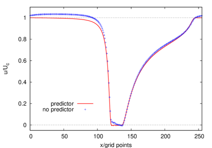
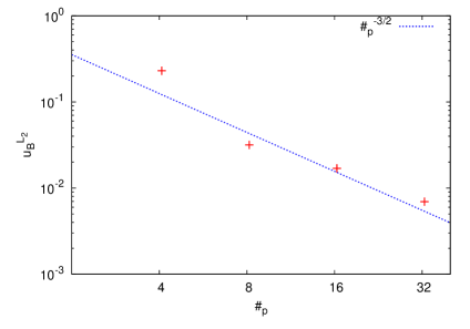
Figure 1: (Left) Profile of the velocity (normalised to the inflow speed) in the direction of the mean flow on the axis of symmetry. The solid line corresponds to a computation with predictor $p^{n-1}$ while the points correspond to a computation without the predictor. (Right) $L_{2}$ norm of the velocity inside the particle as a function of the number of grid points on its diameter

A measure for the accuracy of the boundary conditions is given by the $L_{2}$-norm

$$u_{B}^{L_{2}}=\left(\int_{B}|\bm{u}(x)|^{2}dx\right)^{1/2}$$ (8)

of the velocity inside the fixed spherical particle. This norm is represented in Fig. 1 (Right) for a flow with a particle Reynolds number $\mbox{{Re}}_{\mathrm{p}}=20$ and as a function of the number of grid-points $\#_{p}$ along the diameter of the sphere. This number quantifies the resolution of the geometry of the particle by the underlying homogeneous grid. The norm $u_{B}^{L_{2}}$ shows a power-law decrease with an exponent $-3/2$. This value can be understood by remembering that the fluid velocity field is continous but not differentiable at the surface of the particle. In a spectral scheme, fields are represented by truncated series of $K$ modes. One can then easily show that the singular behavior of $\bm{u}$ at the surface leads to $u_{B}^{L_{2}}\propto K^{-3/2}$.

2.3 The forces on the sphere

The force that is exerted by the fluid on the particle is given by the integral over the surface of the particle of the fluid stress tensor

$$\bm{F}=\int_{\Omega_{\mathrm{p}}(t)}\nabla\cdot\mathbb{T}\,\,\mathrm{d}^{3}x=\int_{\partial\Omega_{\mathrm{p}}(t)}\mathbb{T}\cdot\mathrm{d}\bm{S},\qquad\mbox{where}\quad\mathbb{T}=-p\bm{I}_{3}+\nu\,(\nabla\bm{u}+{\nabla\bm{u}}^{T}).$$ (9)

The torque on the particle is given by

$$\bm{T}=\int_{\partial\Omega_{\mathrm{p}}(t)}\bm{n}\times(\mathbb{T}\cdot\mathrm{d}\bm{S})$$ (10)

where $\bm{n}$ is the unit normal vector of the particle surface. The total force $\bm{F}$ can easily be computed from the penalty force $\bm{f}_{b}$ because

$$\int_{\Omega_{\mathrm{p}}(t)}\nabla\cdot\mathbb{T}\,\,\mathrm{d}^{3}x=\int_{\Omega_{\mathrm{p}}(t)}\bm{f}_{b}\,\mathrm{d}^{3}x.$$

In order to distinguish the pressure and viscous terms appearing in the stress tensor (9), our strategy consists in computing the pressure contribution by constructing a homogeneous grid of points at the sphere surface. Then, we integrate the directed pressure $p\bm{n}$, $\bm{n}$ being the normal vector field at the surface of the particle, over this grid. The viscous part is obtained by subtracting the pressure contribution from the total force.

3 A particle in a laminar upstream flow

We conduct here a numerical wind tunnel experiment, as already described above. The sphere is fixed and the inflow velocity $U_{c}$ is prescribed to be equal to one. The Reynolds number is varied by changing either the particle diametre $d$ or the viscosity of the fluid. The principle flow configuration is depicted in Fig. 2 above the critical Reynolds number where a non-stationary wake develops.

Figure 2: Turbulent wake at $\mbox{{Re}}_{\mathrm{p}}=400$ (volume rendering of high-vorticity isosurfaces).

The goal of such settings is two-fold. First, it is used to perform several benchmarkings of the proposed numerical method. Secondly, it used to investigate the decay of the turbulent wake at moderate Reynolds numbers for which we propose an approach in terms of the “principle of permanence of large eddies”.

3.1 Forces acting on the particle

We first report measurements on the drag-coefficient

$$C_{D}=\frac{8\,F_{D}}{\pi d^{2}\,\rho_{\mathrm{f}}U_{c}^{2}},$$ (11)

where $F_{D}$ denotes the total force exerted on the particle in the stream-wise direction and $\rho_{\mathrm{f}}$ the fluid mass density (set here to one). Figure 3 shows the measured coefficient. Data compare well to Schiller & Naumann (1933) empirical formula

$$C^{\mathrm{SN}}_{D}=\frac{24}{\mbox{{Re}}_{\mathrm{p}}}(1+0.15\mbox{{Re}}_{\mathrm{p}}^{0.687}).$$ (12)

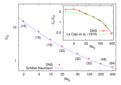
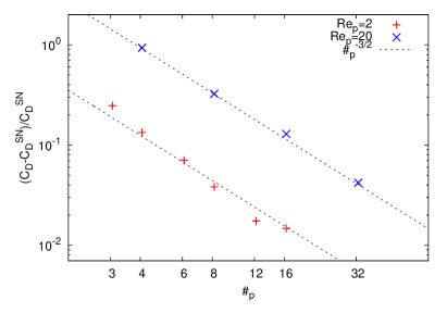
Figure 3: (Left) Drag-coefficients $C_{D}$ as a function of the particle Reynolds number; in parenthesis is given the number of internal grid points. Inset: ratio between the viscous contribution $C_{F}$ to the drag coefficient and the contribution $C_{P}$ from pressure. (Right) Convergence rate as a function of the number of grid points $\#_{p}$ across the sphere.

The numbers in parenthesis in Fig. 3 (Left) denote the number of grid-points $\#_{p}$ across the sphere diametre $d$ and controls the resolution of the boundary layer around the sphere. The thickness of this layer decreases as $\mbox{{Re}}^{-1/2}\,d$. Hence higher is the Reynolds number, more points $\#_{p}$ are required. In order to check to performance of the scheme in the case where the particle is moving, we changed the frame of reference of this experiment and translated the particle in a flow at rest. Also the zone where we remove the velocity fluctuations is moved according to the particle position. The measured drag coefficients and the velocity profile around the sphere are nearly indistinguishable from the former wind tunnel experiments. We observe fluctuating deviations from the values given in Fig. 3 of less than one percent for Reynolds number up to 50 and less than five percent up to 400. The inset of Fig. 3 (Left) shows the ratio of the viscous $C_{F}$ to the pressure $C_{P}$ contribution to the complete drag $C_{D}=C_{F}+C_{P}$. The measured ratios are in reasonable agreement with the results of Le Clair et al. (1970), who used a finite-difference scheme. A possible explanation of the discrepancy could stem from the method we use to separate the viscous and pressure contributions. However, we stress again that such a distinction of these two parts to the total force is not needed for the integration of the particle dynamics and might only be of interest for analysis purposes.

The convergence of the drag coefficient can be quantified by looking at the relative error $(C_{D}-C^{\mathrm{SN}})/C^{\mathrm{SN}}$ as a function of the internal points $\#_{p}$. From Fig. 3 (Right) we observe that the coefficients converge with an exponent of -3/2 for the two Reynolds numbers showed there. This is the same rate of convergence as for the $L_{2}$ norm $u_{B}^{L_{2}}$ of the velocity inside the particle (see previous section), which suggests that the convergence rate of the proposed scheme is determined by the convergence rate of the truncated representation of the $C^{0}$-velocity field.

We next consider a non-homogeneous inflow with a constant gradient $U_{y}=U_{c}+g\,(y-y_{0})$, caracterized by the non-dimensional shear rate $s={g\,d}/{U_{c}}$. This linear velocity profile creates a lift force $F_{L}=\bm{F}\cdot\bm{e}_{y}$ on the particle, whose associated lift coefficient is

$$C_{L}=\frac{8\,F_{L}}{\pi d^{2}\rho_{\mathrm{f}}U_{c}^{2}}.$$ (13)

This coefficient have been measured by different groups: Dandy & Dwyer (1990) used finite volumes, Kurose & Komori (1999) finite differences, and Bagchi & Balachandar (2002) a Chebyshev–Fourier method. All of them used a cylindrical mesh to reach a higher resolution near the particle surface.

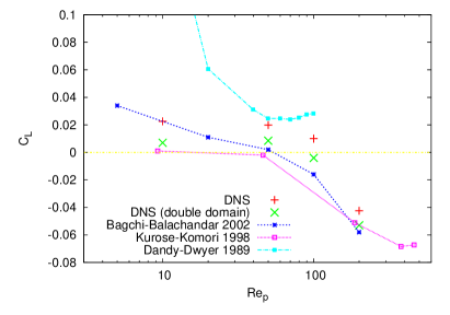
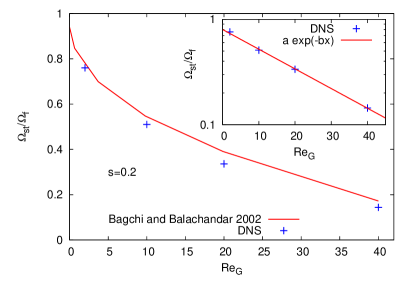
Figure 4: (Left) Lift-coefficients $C_{L}$ as a function of the particle Reynolds number for $s=0.2$. (Right) Stationary rotation rate (normalised to the ambient rotation rate $\Omega_{f}=g/2$) as a function of the particle Reynolds number defined with the mean fluid velocity gradient $\mbox{{Re}}_{\mathrm{G}}=gd^{2}/\nu$. Inset: Logarithmic representation. For the exponential fit we used $a=0.8$ and $b=0.043$.

From Fig 4 (Left) one observes a quite large spread of the lift coefficients measured by these three groups. This is due to the sensitivity of the lift force on the stresses in the flow and thus on the size of the computational domain. It has been claimed by Bagchi & Balachandar (2002) that the box size in the work of Dandy & Dwyer (1990) was too small, leading to an overestimation of the lift force. We have computed the lift force for two different box sizes ($128\!\times\!128\!\times\!256$ and $256\!\times\!256\!\times\!512$) and observe a decreasing force with increasing box-size. Our measurements are in good qualitative agreement with the two most recent works and reproduce in particular the transition to negative values for $\mbox{{Re}}_{\mathrm{p}}\approx 60\!-\!80$. To address in more details this question, larger simulations would be required; this is beyond the scope of this work.

We have finally considered a freely rotating sphere in this shear flow. After a relaxation period, the sphere torque-free rotation rate attains a stationary value, which is shown in Fig. 4 (Right) as a function of the shear rate. The measured values agree well with those of Bagchi & Balachandar (2002). In particular, the decay is slower than the algebraic form proposed by Lin et al. (1970). As seen in the inset, we actually observe that the rotation rate decreases exponentially with the Reynolds number. However, this might again result from a finite-box effect.

We have seen in this section that the drag and lift coefficients in a laminar upstream flow are reasonably well captured by the proposed numerical method. We will now turn to investigating the decay of the turbulent wake. Before this let us do some comments on the effect of Gibbs oscillations on the accuracy of the applied numerical method. The representation of a discontinuous function with a finite number $N/3$ of Fourier modes introduces oscillations in real space. In our case the velocity gradient displays such oscillations whose amplitude decreases as $1/(k_{max}\,x)$ where $x$ is the distance to the particle surface and $k_{max}=(2\pi/L)\,N/3$. As we will see in the next section the velocity gradient in the turbulent wake of the particle decays as $x^{-3/2}$, that is faster than Gibbs oscillations. This implies that there is a distance $x^{*}\simeq C\,k_{max}^{2}$ beyond which the error takes over. This gives some limitations in the use of this method to investigate the very-far wake. Nevertheless, its quadratic dependence on $k_{max}$ makes $x^{*}$ grow fast as a function of the resolution. In addition we expect the constant $C$ to increase with the particle Reynolds number as the gradients get steeper. It is thus very likely that the proposed method is adapted to study small-scale statistics in the turbulent wake for the parameter range of our simulations. Also let us stress that in the case when the outer flow is itself in a developed turbulent state, the gradient has a typical amplitude so that Gibbs oscillations are always sub-dominant at sufficiently far distances.

3.2 Turbulent wake at moderate Reynolds numbers

We now focus on the fluid flow velocity and measure the turbulent velocity statistics in the wake of the particle. Most models for turbulent flows past an obstacle rely on studying solutions to the Reynolds-averaged equations for the stationary average $\bm{U}(\bm{x})=\langle\bm{u}(\bm{x},t)\rangle$ velocity field. This equation involves the Reynolds stress tensor $\tau_{ij}(\bm{x})=\langle u^{\prime}_{i}(\bm{x},t)\,u^{\prime}_{j}(\bm{x},t)\rangle$, where $\bm{u}^{\prime}=\bm{u}-\bm{U}$ denotes here the turbulent fluctuation. It is generally closed using an eddy-viscosity assumption (see, e.g., Pope, 2000). When the eddy viscosity $\nu_{\mathrm{T}}$ is assumed to be constant in space, one obtains that the streamwise mean velocity $U(x,y,z)=\langle u_{x}(\bm{x},t)\rangle$ has the self-similar form (see, e.g., Schlichting, 1979)

$$U(x,y,z)=U_{c}\left[1-\frac{C_{D}\,d^{2}}{32\,\nu_{\mathrm{T}}x}\,\mathrm{e}^{-\frac{y^{2}+z^{2}}{r_{1/2}^{2}(x)}}\right],\mbox{ with }r_{1/2}(x)=d\,\sqrt{\frac{2\,U_{c}\,x}{\nu_{\mathrm{T}}\,\ln 2}}.$$ (14)

$r_{1/2}$ is called the wake half-width. Note that we assume in this section that the particle is located at $x_{0}=0$. Such a formula, which is commonly used in industrial applications, implies that the mean velocity deficit $\Delta U=1-U(x,0,0)/U_{c}$ behaves as $x^{-1}$ at large distances. This law was observed experimentally (Wu & Faeth, 1994) and numerically (Bagchi & Balachandar, 2004).

An analysis of the turbulent wake from a direct simulation performed at the moderate value of the particle Reynolds number $\mbox{{Re}}_{\mathrm{p}}=400$ shows that this similar eddy-viscosity theory rightly predicts the decay of the mean velocity deficit. This is clear in Fig. 5 (Left) where $\Delta U$ decreases like a power law with exponent $-1$ over nearly half a decade. The oscillations around the value $-1$ that we observe for the local slope in the inset are a signature of the Gibbs phenomenon induced by the strip forcing at $x\approx 12d$.

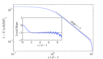
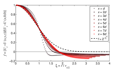
Figure 5: (Left) mean velocity deficit $\Delta U=1-U(x,0,0)/U_{c}$ in the axis of symmetry $y=0$ and $z=0$ of the wake as a function of the normalised streamwise distance $x/d$. The inset represents its logarithmic derivative $[\mathrm{d}\ln\Delta U]/[\mathrm{d}\ln(x/d-1)]$. (Right) mean velocity deficit profile $f$ as a function of the reduced spanwise distance $\xi=r/r_{1/2}$ for various values of $x/d$ as labelled; the bold dashed line represents the Gaussian functional form of $f$ obtained from the constant-eddy-viscosity similar profile (14).

However, as seen from the right-hand panel of Fig. 5, the mean velocity deficit profile does not seem to display any similarity. The half width $r_{1/2}$ was computed as the value of the distance to the axisymmetric axis where the velocity deficit is equal to $1/2$. One observes discrepancies for values of the reduced variable $\xi=r/r_{1/2}=\sqrt{y^{2}+z^{2}}/r_{1/2}$ that are close to $1/2$, to $3/2$, and for $\xi>2$. The deviation at large $\xi$’s might be due to the periodicity of the spatial domain in the $y$ and $z$ directions. However the deviations at moderate values are comparable to those obtained experimentally by Uberoi & Freymuth (1970) and Wu & Faeth (1994).

In order to get a better handling on the observed $\propto x^{-1}$ behaviour, we relate it now to the decay of turbulent kinetic energy in the wake of the particle. For this, we introduce an original approach based on the “principle of permanence of large eddies” that is known since the seminal work of Kolmogorov (1941) for the time decay of homogenous turbulence. We refer here the reader to the phenomenological presentation of this law made by Frisch (1995). The principle of permanence of large eddies states that if the initial turbulent velocity correlations have the form $\langle u(x+r)\,u(x)\rangle\sim r^{-h}$ at large scales $r$, the decay behaviour of all turbulent quantities is dictated by the value of the exponent $h$. In particular, the integral scale is $L\sim t^{1/(1+h)}$ and the kinetic turbulent energy behaves as $k\sim t^{-2h/(1+h)}$. The main principle used in this approach is the continuity of correlations at $r=L$.

When considering the decay of wake turbulence, all the turbulent quantities have to be of course evaluated in planes perpendicular to the axisymmetric axis and time has to be replaced by $x/U_{c}$ by invoking Taylor hypothesis. Also, instead of using continuity at separations equal to the correlation length, the main ingredient is here that the spatial correlations of turbulent fluctuations have to match the decay of the velocity deficit at very large transverse distances $r$. The principle of permanence of large eddies then implies that if the velocity deficit $\Delta U(r)$ at a distance $r$ from the axis of symmetry behaves as $r^{-h}$ in the developing wake, then at any $x>0$ in the far wake, the large-scale correlations of the turbulent fluctuations should remember this initial form and the turbulent kinetic energy is expected to decay as $k\sim x^{-2h/(1+h)}$.

We now give an argument demonstrating that the velocity deficit decays exponentially at large transverse distances $r$. For that, we assume that, to leading order, the axisymmetric mean velocity profile takes for $r\gg d$ the separated form

$$U_{\parallel}\simeq U_{c}+\Phi_{\parallel}(r)\,\Psi_{\parallel}(x)\quad\mbox{and}\quad U_{\perp}\simeq\Phi_{\perp}(r)\,\Psi_{\perp}(x),$$ (15)

in the streamwise and transverse directions, respectively. We choose here $\Phi_{\parallel}>0$ and $\Phi_{\perp}>0$, so that $\Psi_{\parallel}<0$ and $\Psi_{\perp}<0$. Incompressibility implies $\Phi_{\parallel}\Psi_{\parallel}^{\prime}+(1/r)\,(r\Phi_{\perp})^{\prime}\,\Psi_{\perp}=0$, so that

$$(r\Phi_{\perp})^{\prime}=C_{1}\,r\,\Phi_{\parallel}\quad\mbox{and}\quad\Psi_{\parallel}^{\prime}=-C_{1}\,\Psi_{\perp},$$ (16)

where $C_{1}$ is a constant, which by dimensional analysis should be $\propto 1/d$. To leading order, the stationary Navier–Stokes equation yields

$$U_{c}\,\Phi_{\parallel}\,\Psi_{\parallel}^{\prime}\simeq-\partial_{x}p\quad\mbox{and}\quad U_{c}\,\Phi_{\perp}\,\Psi_{\perp}^{\prime}\simeq-\partial_{r}p.$$ (17)

The leading behaviour of the non-linear term is here given by the advection of the perturbed velocity by the mean flow $U_{c}$. Note that the Reynolds stress involves the square of the turbulent fluctuations and is thus subleading when $r\gg d$. As the viscous terms become negligible at large distances, advection is exactly compensated by the pressure gradient. We now equate the second-order cross derivative $\partial_{x}\partial_{r}p$ of pressure obtained from these two equations to write $\Phi_{\parallel}^{\prime}\Psi_{\parallel}^{\prime}=\Phi_{\perp}\Psi_{\perp}^{\prime\prime}$, leading to

$$\Phi_{\parallel}^{\prime}=C_{2}\,\Phi_{\perp}\quad\mbox{and}\quad\Psi_{\perp}^{\prime\prime}=C_{2}\,\Psi_{\parallel}^{\prime},$$ (18)

where again $C_{2}$ is a constant $\propto 1/d$. Put together, the conditions (16) and (18) imply that $r\Phi_{\perp}$ is a solution of the differential equation

$$(r\Phi_{\perp}^{\prime})^{\prime}=C_{1}\,C_{2}\,r\,\Phi_{\perp},\quad\mbox{so that}\quad\Phi_{\perp}\propto\frac{1}{\sqrt{r}}\,\mathrm{e}^{-C\,r/d},\mbox{ when }r\gg d$$ (19)

with $C=d\,\sqrt{C_{1}\,C_{2}}$ a positive dimension-less constant that is independent of $d$. This exponential decay of the mean velocity deficit implies the same behavior for velocity correlations, as confirmed numerically. We indeed see in Fig. 6 (a) that, for various values of $x$, the correlations of the radial component of the fluctuating velocity collapse for large $r$ to an exponential behaviour $\propto\exp(-r/r_{0})$. To our knowledge this behaviour has never been observed before.

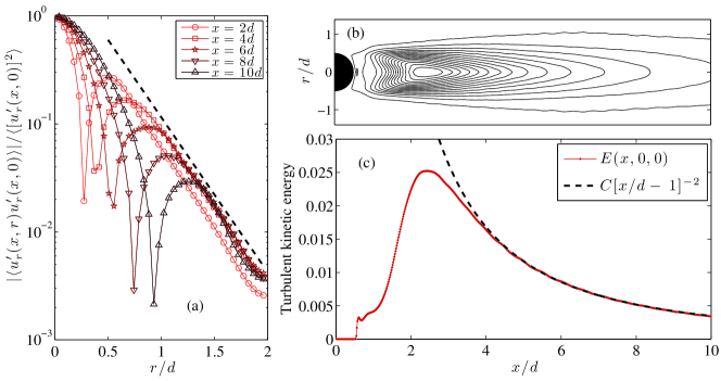
Figure 6: (a) Correlation of the velocity radial fluctuation as a function of the distance $r$ to the axisymmetric axis for various values of the streamwise distance $x$ as labelled; the dashed line corresponds to an exponential decay. (b) Contour lines of the turbulent kinetic energy $k$ in the $(x,r)$ plane. (c) Profile of $k$ along the $r=0$ axis, clearly displaying a behaviour $\propto x^{-2}$

Turnig back to the law of decay, an exponential behaviour of correlations corresponds to $h=\infty$. This implies that the turbulent kinetic energy decays as $k\sim x^{-2}$, as confirmed numerically in Fig. 6 (c). Such a law of turbulence decay can in turn be related to the downstream decrease of the velocity deficit. The Reynolds-averaged Navier–Stokes equation can be used to show that $\Delta U(x)=1-U(x,0,0)/U_{c}$ approximately obeys

$$U_{c}^{2}\,\partial_{x}\Delta U\sim\partial_{x}\tau_{xx}+\partial_{y}\tau_{xy}+\partial_{z}\tau_{xz}\sim k/L\propto x^{-2},\qquad\mbox{so that}\quad\Delta U\sim x^{-1}.$$ (20)

$\bm{\tau}$ denotes here the Reynolds stress tensor. This finally implies that the scaling of the velocity deficit is consistent with the decay of turbulent kinetic energy. Also $h=\infty$ implies that the integral scale remains constant ($L\sim x^{0}$). The kinetic energy dissipation rate is thus decreasing as $\varepsilon\sim k^{3/2}/L\sim x^{-3}$, so that the typical turbulent gradients behave as $\partial_{x}u\sim(\varepsilon/\nu)^{1/2}\sim x^{-3/2}$.

We have seen in this section that the numerical method we are using is well adapted to describe the turbulent wake downstream the particle. This is for instance supported by the accuracy with which the decay laws are measured. This can be understood by the fact that Fourier-spectral methods are well adapted to simulations of developed turbulence. To take advantage of this, we next turn to investigating the influence of turbulent fluctuations that are possibly present in the upstream flow.

4 A particle in a turbulent upstream flow

We now consider that the fluid flow surrounding the particle is forced to sustain a turbulent state. The simulations were set up in the following way: first we precomputed a homogeneous, isotropic turbulent flow in a periodic box without particle by solving (1) with $\Omega_{p}=\emptyset$. A statistically stationary flow is reached by keeping constant the energy content in the two lowest Fourier shells of the velocity field. On this turbulent flow we superimposed a constant mean flow $\bm{U}_{c}=U_{c}\,\bm{e}_{x}$ by keeping constant the real part of the zero Fourier mode. Afterwards, a fixed sphere is placed into this fluctuating stream by means of the penalty method discussed above. We thus solve (1) with (2) in a periodic domain while choosing its size sufficiently large in the streamwise direction so that the sphere does not interact with its own wake. The upstream flow seen by the sphere can therefore be considered homogeneous and isotropic. We have performed four series of numerical simulations corresponding to four different particle Reynolds numbers $\mbox{{Re}}_{\mathrm{p}}$ (defined with the mean flow $U_{c}$). From the range considered in previous section we choose $\mbox{{Re}}_{\mathrm{p}}=20$, $\mbox{{Re}}_{\mathrm{p}}=100$, $\mbox{{Re}}_{\mathrm{p}}=200$, and $\mbox{{Re}}_{\mathrm{p}}=400$ in order to cover three qualitatively different wake configurations. For $\mbox{{Re}}_{\mathrm{p}}=20$ the wake is intrinsically laminar without any recirculation region behind the particle, for $\mbox{{Re}}_{\mathrm{p}}=100$ and $\mbox{{Re}}_{\mathrm{p}}=200$ a laminar recirculation region develops and for $\mbox{{Re}}_{\mathrm{p}}=400$ the wake becomes intrinsically turbulent. The parameters of the simulations are given in table 1.

$\mbox{{Re}}_{p}$	Re	$u_{\mathrm{rms}}$	$\varepsilon$	$\nu$	d	$\eta$	$\tau_{\eta}$	$L$	$T_{L}$	$N^{3}$
20	$0$	$0$	$1.7\cdot 10^{-4}$	0.02	0.4	$-$	$-$	$-$	$-$	$1024\times 256^{2}$
20	$0.31$	$0.05$	$4.7\cdot 10^{-4}$	0.02	0.4	(0.36)	(6.5)	(0.15)	(3.7)	$1024\times 256^{2}$
20	$0.94$	$0.064$	$6.4\cdot 10^{-4}$	0.02	0.4	(0.34)	(5.5)	(0.32)	(5.4)	$1024\times 256^{2}$
20	$3.2$	$0.12$	$2.64\cdot 10^{-3}$	0.02	0.4	$0.24$	2.85	0.56	4.9	$1024\times 256^{2}$
20	$23$	$0.27$	$1.23\cdot 10^{-2}$	0.02	0.4	$0.16$	1.38	1.67	6.1	$1024\times 256^{2}$
20	$39$	$0.37$	$2.40\cdot 10^{-2}$	0.02	0.4	$0.135$	0.91	2.11	5.7	$1024\times 256^{2}$
20	$78$	$0.57$	$6.65\cdot 10^{-2}$	0.02	0.4	$0.11$	0.55	2.75	4.9	$1024\times 256^{2}$
100	0	0	$1.5\cdot 10^{-4}$	0.006	0.6	$-$	$-$	$-$	$-$	$1024\times 256^{2}$
100	49.1	0.135	$1.13\cdot 10^{-3}$	0.006	0.6	0.11	2.14	2.18	16.1	$1024\times 256^{2}$
100	140	0.28	$7.3\cdot 10^{-3}$	0.006	0.6	0.074	0.90	3.01	10.7	$1024\times 256^{2}$
100	288	0.58	$6\cdot 10^{-2}$	0.006	0.6	0.043	0.32	2.93	4.97	$1024\times 256^{2}$
200	0	0	$5.4\cdot 10^{-5}$	0.003	0.6	$-$	$-$	$-$	$-$	$2048\times 256^{2}$
200	130	0.135	$8.5\cdot 10^{-4}$	0.003	0.6	$0.075$	$1.85$	2.89	21.4	$2048\times 256^{2}$
200	305	0.28	$6.7\cdot 10^{-3}$	0.003	0.6	$0.045$	$0.67$	3.28	11.7	$2048\times 256^{2}$
200	426	0.4	$2.0\cdot 10^{-2}$	0.003	0.6	$0.034$	$0.39$	3.20	8.0	$2048\times 256^{2}$
400	0	0	$7.5\cdot 10^{-5}$	0.002	0.8	$0.102$	$5.2$	$-$	$-$	$2048\times 256^{2}$
400	46.1	0.061	$1.5\cdot 10^{-4}$	0.002	0.8	$0.086$	$3.7$	1.51	24.81	$2048\times 256^{2}$
400	65.0	0.0714	$2.0\cdot 10^{-4}$	0.002	0.8	$0.079$	$3.15$	1.82	25.49	$2048\times 256^{2}$
400	203	0.139	$9.2\cdot 10^{-4}$	0.002	0.8	$0.054$	$1.46$	2.92	21.0	$2048\times 256^{2}$
400	434	0.286	$7.7\cdot 10^{-3}$	0.002	0.8	$0.032$	$0.51$	3.04	10.63	$2048\times 256^{2}$
400	605	0.392	$1.95\cdot 10^{-2}$	0.002	0.8	$0.025$	$0.32$	3.09	7.88	$2048\times 256^{2}$
400	927	0.598	$6.9\cdot 10^{-2}$	0.002	0.8	$0.018$	$0.17$	3.10	5.18	$2048\times 256^{2}$

Table 1: Parameters of the numerical simulations. $\mbox{{Re}}_{\mathrm{p}}=U_{c}\,d/\nu$, $\mbox{{Re}}=u_{\mathrm{rms}}L/\nu$: Reynolds number, $u_{\mathrm{rms}}$: root-mean-square velocity, $\varepsilon$: mean kinetic energy dissipation rate, $\nu$: kinematic viscosity, $d$: sphere diameter, $\eta=(\nu^{3}/\varepsilon)^{1/4}$: Kolmogorov dissipation length scale, $\tau_{\eta}=(\nu/\varepsilon)^{1/2}$: Kolmogorov time scale, $L=u_{\mathrm{rms}}^{3}/\varepsilon$: integral scale, $T_{L}=L/u_{\mathrm{rms}}$: large-eddy turnover time, $N^{3}$: number of collocation points.

The physical configuration is determined by three dimensionless parameters: the particle Reynolds number $\mbox{{Re}}_{\mathrm{p}}$, the Reynolds number of the fluid Re, and the turbulent large-scale intensity $I=u_{\mathrm{rms}}/U_{c}$. The latter measuring the strength of the large scale turbulent fluctuations compared to the mean flow velocity. For each particle Reynolds number $\mbox{{Re}}_{\mathrm{p}}$ considered we varied the turbulent intensity $I$ between 0.05 and 0.60. Although the parameter space is three-dimensional we vary only two parameters namely $\mbox{{Re}}_{\mathrm{p}}$ and $I$. This is due to our particular choice of keeping constant, for each value of $\mbox{{Re}}_{\mathrm{p}}$, the mean velocity $U_{c}$, the viscosity $\nu$, the particle diameter $d$ and the form of the external forcing but to vary only its amplitude. This latter control parameter determines in turn the root-mean-square velocity $u_{\mathrm{rms}}$, which enters in the definitions of both $I$ and Re.

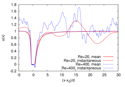
Figure 7: Left: Instantaneous velocity profile, together with its temporal average; the sphere center is here located at $x_{0}$. Right: averaged velocity profiles for $\mbox{{Re}}_{\mathrm{p}}=400$ and various values of the turbulent intensity $I$ as labelled.

A first qualitative idea of the flow structure around the sphere can be observed from Fig. 7 (Left) where instantaneous velocity profiles along the axis of symmetry, together with their temporal averages, are shown for two particle Reynolds numbers ($\mbox{{Re}}_{\mathrm{p}}=20$ and $\mbox{{Re}}_{\mathrm{p}}=400$) in the case of a turbulent intensity $I\approx 0.25$. From the instantaneous profiles we remark that, for a given turbulent intensity, the higher is the particle Reynolds number, the smaller are the typical lengthscales of the turbulent fluctuations. Also, when fixing $\mbox{{Re}}_{\mathrm{p}}=400$ and varying the intensity $I$, we see in Fig. 7 (Right) that stronger turbulent fluctuations reduce the extent of the mean particle wake. This confirms observations made by Bagchi & Balachandar (2004).

4.1 The drag and lift forces

We computed the mean drag, i.e. the force exerted by the turbulent flow on the particle in the streamwise direction (the averaged perpendicular forces are zero). The total force acting on the particle also contains the volume forcing applied to maintain the carrier flow in a stationary turbulent state. However, we have estimated this force and could show that its contribution is negligible compared to the drag and lift forces exerted by the fluid. Results are shown in Fig.8 (Left), where data is normalised to the case without turbulent fluctuations. The error bars are given by measuring the standard deviation from the mean and estimating how many independent realisations our temporal signal contains. For that we approximate the correlation time by the zero-crossing time of the auto-correlation functions of the drag forces (see later).

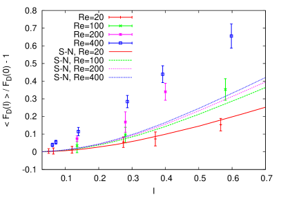
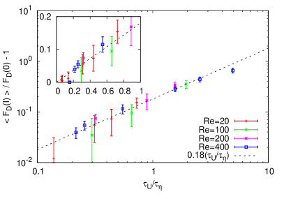
Figure 8: Left: deviations of the mean drag from that obtained with a laminar upstream flow as a function of the turbulent intensity $I$. Right: same represented as a function of the ratio $\tau_{\mathrm{U}}/\tau_{\eta}$ where $\tau_{\mathrm{U}}=d/U_{c}$ is the sweeping time over a distance equal to the particle diameter and $\tau_{\eta}=(\nu/\varepsilon)^{1/2}$ is the turbulent turnover time associated with the Kolmogorov dissipative scale $\eta$.

One finds a clear increase of the stream-wise force on the particle with increasing turbulent intensity. For instance, when $\mbox{{Re}}_{\mathrm{p}}=400$ and $I=0.5$, we measure a relative increase of 40%. Indications for this increased drag were already given by Bagchi & Balachandar (2003) and Kim & Balachandar (2012). However, their turbulent intensities were too small and the error-bars were too large to clearly distinguish their measured drag from the drag obtained without turbulence and validate undoubtedly the observed increase.

As stated in Bagchi & Balachandar (2003), it is very likely that the drag increase is due to the non-linear dependence of the drag upon the incident fluid velocity. The instantaneous slip velocity of the particle is given by $\bm{U}=U_{c}\,\bm{e}_{x}+\mathcal{U}$ where the large-scale turbulent velocity $\mathcal{U}$ can be approximated by a Gaussian random vector with zero mean and variance $u_{\mathrm{rms}}^{2}$. The fluctuations of $\mathcal{U}$ can be responsible for an increase of the force $\bm{F}$. Indeed, let us assume that the relation between $\bm{F}$ depends and $\bm{U}$ is instantaneously given by the Schiller and Naumann approximation formula (12), that is

$$\bm{F}\approx\bm{F}^{\mathrm{SN}}(\bm{U})=3\pi\,d\,\nu\left[1+0.15\left(\frac{|\bm{U}|\,d}{\nu}\right)^{\!0.687}\right]\,\bm{U}.$$ (21)

The average of this force with respect to the symmetric Gaussian fluctuations of $\mathcal{U}$ is aligned with the streamwise direction $x$ and reads

$$\overline{\bm{F}}^{\mathrm{SN}}(I) = \frac{1}{\left(\sqrt{2\pi}\,u_{\mathrm{rms}}\right)^{3}}\int\bm{F}^{\mathrm{SN}}(\bm{U})\,\mathrm{e}^{-|\mathcal{U}|^{2}/(2u_{\mathrm{rms}}^{2})}\,\mathrm{d}^{3}\mathcal{U}$$ (22)

$$= 3\pi\,d\,\nu\,U_{c}\,\bm{e}_{x}\left[1+\frac{0.15\,\mbox{{Re}}_{\mathrm{p}}^{0.687}}{(2\pi)^{3/2}}\!\!\int(1\!+\!I\,v_{1})|\bm{e}_{x}\!+\!I\,\bm{v}|^{0.687}\,\mathrm{e}^{-|\bm{v}|^{2}/2}\,\mathrm{d}^{3}v\right]\!\!.$$

Although the integral cannot be written explicitly, one can easily check that it leads to a relative increase of the drag that takes of the form $\Delta^{\mathrm{SN}}(I)=\overline{F}^{\mathrm{SN}}(I)/\overline{F}^{\mathrm{SN}}(0)-1\simeq C\,I^{2}$ where $C\approx 0.45\,\mbox{{Re}}_{\mathrm{p}}^{0.687}/(1+0.15\,\mbox{{Re}}_{\mathrm{p}}^{0.687})>0$. Also, the estimate (22) does surprisingly not depend on the fluid Reynolds number Re but only on the two other dimensionless parameters $I$ and $\mbox{{Re}}_{\mathrm{p}}$. The prediction (22) is shown as lines in Fig. 8 (Left). While it gives a rather good approximation of the data at moderate particle Reynolds numbers, it is clearly a too low estimate for $\mbox{{Re}}_{\mathrm{p}}>100$. The discrepancy might be due to the impossibility for this approach to account for the dependence on Re.

Another heuristic way to understand the effect of the perturbing turbulence on the drag consists in considering the modification of the amplitude of the typical velocity gradient in the neighbourhood of the particle. In the laminar case (when $I=0$), the velocity field around the particle typically varies over a scale of the order of $d$. The unperturbed gradient is then $\sim U_{c}/d$. When a background turbulence is added to this flow, the value of the gradient is modified by the typical turbulent gradient $u_{\eta}/\eta=\tau_{\eta}^{-1}=\nu^{-1/2}\varepsilon^{1/2}$ where $\tau_{\eta}$ is the turnover time associated to the Kolmogorov dissipative scale $\eta$. The velocity gradients appear in the viscous forces acting on the particle and also at leading order on the pressure gradient via the Poisson equation. Altogether these considerations imply that the corrections to the drag are expected to be $\propto\tau_{\eta}^{-1}$, while these forces in the $I=0$ reference case should be $\propto\tau_{U}^{-1}$, where $\tau_{U}=d/U_{c}$. Such arguments leads to a relative increase $\Delta(I)$ of the drag force acting on the particle $\propto\tau_{U}/\tau_{\eta}=I^{2}\mbox{{Re}}_{\mathrm{p}}\,\mbox{{Re}}^{-1/2}$. The right-hand side of Fig. 8 shows $\Delta(I)$ as a function of $\tau_{U}/\tau_{\eta}$ and reveals a rather good collapse of the entire dataset to the curve $\Delta(I)=0.18\,(\tau_{U}/\tau_{\eta})$, giving support to such phenomenological arguments. Notice that this approach gives again a behaviour $\propto I^{2}$ for small values of the turbulence intensity, but with this time a constant that depends explicitly on the outer-flow Reynolds number Re.

There are thus at least two different mechanisms that explain the drag increase by the impacting turbulence: The non-linear dependence of the drag on the incident large-scale velocity and the modification of the particle boundary layer by small-scale turbulent fluctuations. These two effects might act concomitantly at small turbulent intensities. However, data show that the drag increase strongly depends on the particle Reynolds number. This effect is not captured by the first approach. In addition the collapse of data in Fig. 8 (Right) gives support to the importance of shear effects. Nevertheless, one cannot firmly favour one of these two mechanisms as the qualitative consequences of an outer turbulence depend on the particle Reynolds number.

An instance of differing behaviours depending on $\mbox{{Re}}_{\mathrm{p}}$ is the ratio between the respective contributions $F_{p}$ and $F_{v}$ of pressure and viscosity to the drag. We show in the left-hand side of Fig. 9 their normalised ratio $\alpha(I)=\langle F_{p}(I)\rangle/\langle F_{v}(I)\rangle$ for different turbulent intensities. For the lowest particle Reynolds number ($\mbox{{Re}}_{\mathrm{p}}=20$), the pressure contribution to the total force increases with the turbulent intensity while one observes the opposite for the highest Reynolds number ($\mbox{{Re}}_{\mathrm{p}}=400$). At the intermediate configuration with $\mbox{{Re}}_{\mathrm{p}}=100$ this ratio is more or less independent of the turbulent intensity. Recall that when $\mbox{{Re}}_{\mathrm{p}}\lesssim 100$ the viscosity contribution is dominant while when $\mbox{{Re}}_{\mathrm{p}}\gg 1$ the pressure largely dominates the drag force. The viscosity and pressure give approximately equal contributions for a particle Reynolds number of 100 (see also the inset of Fig. 3). It seems from our data that the presence of turbulent fluctuations counterbalances these pressure-viscosity ratios which depend on $\mbox{{Re}}_{\mathrm{p}}$. We will see in the following section that the reason for this can be found in the modification of the flow structure around the sphere by the fluctuating nature of the ambient flow at small scales.

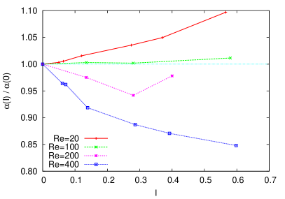
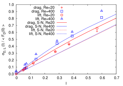
Figure 9: Left: normalised ratio $\alpha(I)=\langle F_{p}(I)\rangle/\langle F_{v}(I)\rangle$ of pressure to viscous contributions to the drag force. Right: standard deviation of the drag force $\sigma_{D}(I)=\langle[F_{D}(I)-\langle F_{D}(I)\rangle]^{2}\rangle^{1/2}$ and of the lift force $\sigma_{L}(I)=\langle[F_{L}(I)-\langle F_{L}(I)\rangle]^{2}\rangle^{1/2}$ as a function of the turbulent intensity. In each case it is normalized to the mean value of the drag force for zero turbulent intensity. The solid lines correspond to the prediction obtained from a fluctuating Schiller–Naumann relation.

After having examined the average forces we now turn to the fluctuations of the drag and lift forces. Their amplitudes can be characterised by their standard deviation, which is shown in the right-hand side of Fig. 9. We observe that the standard deviation increases with increasing turbulent intensity. The fluctuations of the lift forces are slightly larger than those of the drag, as also observed by Bagchi & Balachandar (2003). As the upstream flow is isotropic this difference can only be attributed to the boundary layer of the sphere and its wake. Using the approach described above we used Schiller–Naumann relation for the drag to derive a formula equivalent to (22) but for the force standard deviation. The resulting predictions are plotted as solid lines in Fig. 9 (Right). Interestingly, this approach gives a reasonable prediction, indicating that the force fluctuations are mainly due to large-scale fluctuations. We will come back to this conclusion in the following section.

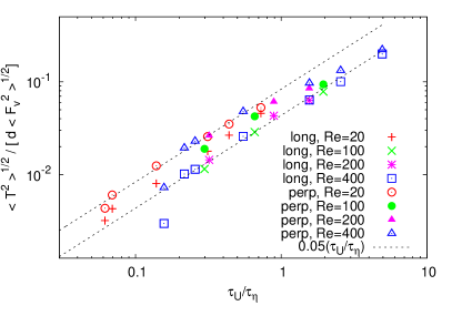
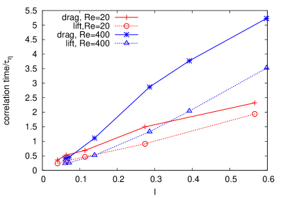
Figure 10: Left: standard deviation of the component of the torque exerted by the flow onto the particle as a function of the ratio $\tau_{U}/\tau_{\eta}$. The streamwise (long) and the spanwise (perp) components show different behaviours. Right: correlation times of the drag and lift forces (see text for definition).

The measured standard deviation of the torque acting on the particle (10) is shown in Fig. 10. There we have normalised it to what we expect to be its typical value, namely the typical amplitude of the viscous force multiplied by the particle diameter $d$. Interestingly, we observe an increase of the torque as a function of the ratio of gradients $\tau_{U}/\tau_{\eta}$. The datapoints collapse to a linear behaviour as a function of $\tau_{U}/\tau_{\eta}$, with a constant that depends whether streamwise or span-wise fluctuations are considered. As for the average drag, the explanation of this linear behaviour relies on the fact that the fluctuations of viscous forces are directly related to the turbulent velocity gradients that surround the particle. We mention that the torque in the stream-wise direction is always smaller than in the transverse directions. Let us also stress that the particle is not allowed to rotate.

We now turn to the two-time statistics of the force exerted by the fluid on the particle by measuring the temporal correlations $C(t)=\langle F(t)\,F(0)\rangle$ of the drag $F_{D}$ and of the lift $F_{L}$. The correlations of the drag always last longer than those of the lift. This property has also been observed in Kim & Balachandar (2012) and can be interpreted by the fact that the drag is more sensitive to large-scale fluctuations, while the lift samples shorter timescales. To quantify this effect, we introduce the correlation time $\tau_{c}$ as the time needed to half the correlation of the forces, i.e. $C(\tau_{c})=(1/2)\,C(0)$. The behaviour of this correlation time as a function of $I$ is shown in the right-hand side of Fig. 10 for $\mbox{{Re}}_{\mathrm{p}}=20$ and $\mbox{{Re}}_{\mathrm{p}}=400$. This graph shows clearly the increase mentioned above.

We also present measurements on the frequency spectrum of the drag and lift forces. For the low-$\mbox{{Re}}_{\mathrm{p}}$ case no difference can be observed between the drag and lift components (not shown). For $\mbox{{Re}}_{\mathrm{p}}=400$, a couple of remarkable features can be observed in Fig. 11 (Left), which shows the amplitudes of the forces Fourier modes as a function of the Strouhal number $\mbox{{St}}=f\,d/U_{c}$, where $f$ is the frequency. In order to reduce the statistical noise we applied a window average. At $\mbox{{Re}}_{\mathrm{p}}=400$ the wake is intrinsically turbulent and we observe a peak in the spectrum at at $\mbox{{St}}^{\star}=0.2$ for the lift force at $I=0$, which matches the eddy-detachment frequency of the wake. Such a peak is not visible for the drag amplitude (not shown). It can be more clearly seen from the inset which shows the ratio of the lift and the drag amplitudes. Two observations deserve attention: first, an increasing turbulent intensity slightly increases this detachment frequency, thus $St^{\star}=St^{\star}(I)$. Secondly, the signature of this frequency survives up to a turbulent intensity of at least 0.29. This is surprising as the amplitude of the turbulent fluctuations at this intensity is larger than the peak-value $F_{D}(St^{\star})$ of a laminar inflow. This means that the turbulent fluctuations increase the violence with which vortex are detached in the wake. This can be related to the increase of the gradients in the mean velocity profile and thus to the shortening of the particle wake that is studied with more details in next section.

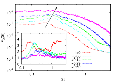
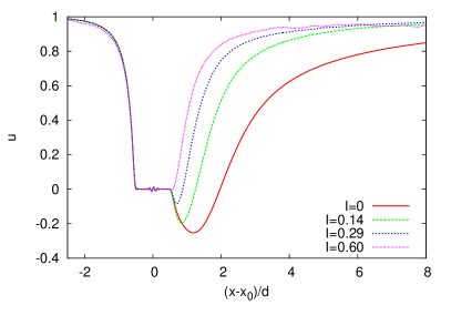
Figure 11: Left: frequency spectrum of the lift forces on the particle as a function of the Strouhal number $\mbox{{St}}=f\,d/U_{c}$. Inset: ratio of the lift to the drag amplitude. Right: half-wake length $l_{1/2}$ defined as $u(l_{1/2})=1/2U_{c}$ and size of the recirculation region $l_{0}$ defined as $u(l_{0})=0$.

4.2 Average velocity boundary layer and wake

As already stated, the particle wake is shortened by the presence of upstream turbulent fluctuations. To quantify this, we measure the half-wake length $l_{1/2}$, which is the distance from the centre of the sphere of the location where the average velocity deficit on the symmetry axis is equal to one half. Data is shown in Fig. 11 (Right). Already a turbulent intensity of 0.3-0.4 is sufficient in both cases to divide by two the size of the laminar wake. Notice that these wake reductions can have important consequences for the interaction between many particles in particle-laden problems, such as sedimentation. We also note that for turbulent intensities larger than 0.2 the wake size normalised by $d$ reaches a behaviour that is identical for all the particle Reynolds numbers considered.

The observed steepenings of the mean velocity gradients in the downstream neighbourhood of the particle are consistent with the results reported previously on the increase of the drag force. Such sharp gradients increase the stress, which leads in turn to an increased viscous drag force — see (9). The average pressure profile around the sphere is also modified by stronger average velocity gradients. The down-stream surface pressure decreases as a function of the turbulent intensity while the up-stream pressure remains almost unchanged (not shown). Thus, the pressure contribution to the drag force also increases with the turbulent intensity. However, we remark that the ratio of these contributions depends on the turbulent intensity (see the left-hand side of Fig. 9).

To understand more quantitatively the modifications of the wake by the turbulent perturbations when $I\ll 1$, let us decompose the velocity field as $\bm{u}=\bm{u}_{0}+\bm{u}^{\prime}$, where $\bm{u}_{0}$ is the velocity obtained in the case of a laminar upstream flow (i.e. when $I=0$), which contains the possible tubulent wake of the particle, and $\bm{u}^{\prime}$ denotes the perturbation due to inflow turbulence (i.e. $\bm{u}^{\prime}=0$ when $I=0$). When averaging with respect to the turbulent fluctuations, the mean velocity profile will be the sum of the unpertubed mean profile $\bm{U}_{0}=\overline{\bm{u}_{0}}$ and of the averaged perturbation $\bm{U}^{\prime}=\overline{\bm{u}^{\prime}}$, which vanishes only far away from the particle. One can easily check writing the Reynolds-averaged equation that, to leading order in $I$, these velocities satisfy

$$\bm{U}^{\prime}\cdot\nabla\bm{U}_{0}+\bm{U}_{0}\cdot\nabla\bm{U}^{\prime}-\nu\nabla^{2}\bm{U}^{\prime}=-\nabla\cdot\bm{\tau}^{\prime}+\nabla P^{\prime},\quad\nabla\cdot\bm{U}^{\prime}=0,$$ (23)

where $\bm{\tau}^{\prime}$ is the Reynolds stress tensor defined as $\tau_{ij}=\overline{u_{i}^{\prime}\,u_{j}^{\prime}}$ and $P^{\prime}$ is the correction to the mean pressure due to the presence of upstream turbulence. As we see from (23) the perturbation $\bm{U}^{\prime}$ of the mean velocity profile originates from the Reynolds stress. The pressure just appears to maintain the divergence-free condition.

Let us estimate the order of magnitude of the different terms appearing in (23). It is clear that $\bm{U}_{0}$ is of the order of the mean upstream velocity $U_{c}$ and that it varies on scales of the order of the particle diameter $d$. The mean perturbation $\bm{U}^{\prime}$ has an unknown amplitude $U^{\prime}$ that we want to characterise. Also, $\bm{U}^{\prime}$ varies over a scale $\ell$ that is different from $d$. To estimate this scale, let us do the following observation. We expect all the turbulent eddies of scales $r\lesssim d$ to be affected in the vicinity of the particle by its presence. While they are swept downstream the particle, we expect the eddies of size $r$ to recover their usual turbulent characteristics after a time of the order of their correlation time $\tau_{r}$. Kolmogorov’s 1941 scaling gives for $r$ inside the inertial range $\tau_{r}\sim\varepsilon^{-1/3}r^{2/3}$, where $\varepsilon$ is the turbulent kinetic energy dissipation rate. The scale $\ell$ of variation of the perturbed wake $U^{\prime}$ is given by the distance downstream the particle that is travelled by the largest perturbed eddies before forgetting they have met the particle. One then distinguishes two cases depending whether $d$ is larger or smaller than the dissipative scale $\eta$ of upstream turbulence. With such phenomenological considerations,

• When $d\gg\eta$, we have $\ell\sim U_{c}\,\tau_{d}\sim U_{c}\,\varepsilon^{-1/3}d^{2/3}$, so that $\ell/d\sim I^{-4/3}\mbox{{Re}}^{1/3}\mbox{{Re}}_{\mathrm{p}}^{-1/3}$. One can then estimate the magnitude of the terms present in the left-hand side of (23):

  $$\bm{U}^{\prime}\cdot\nabla\bm{U}_{0} \sim U^{\prime}\,U_{c}/d,$$

  $$\bm{U}_{0}\cdot\nabla\bm{U}^{\prime} \sim U_{c}\,U^{\prime}/\ell\sim(U^{\prime}\,U_{c}/d)(d/\ell)\sim(U^{\prime}\,U_{c}/d)\,I^{4/3}\mbox{{Re}}^{-1/3}\mbox{{Re}}_{\mathrm{p}}^{1/3},$$

  $$\nu\nabla^{2}\bm{U}^{\prime} \sim \nu\,U^{\prime}/\ell^{2}\sim(U^{\prime}\,U_{c}/d)(d/\ell)^{2}\mbox{{Re}}_{\mathrm{p}}^{-1}\sim(U^{\prime}\,U_{c}/d)\,I^{8/3}\mbox{{Re}}^{-2/3}\mbox{{Re}}_{\mathrm{p}}^{-1/3},$$

  $$\nabla\cdot\bm{\tau} \sim u_{\mathrm{rms}}^{2}/\ell\sim(U_{c}^{2}/d)\,I^{10/3}\mbox{{Re}}^{-1/3}\mbox{{Re}}_{\mathrm{p}}^{1/3}.$$ (24)

  For $\mbox{{Re}}\gg 1$, $\mbox{{Re}}_{\mathrm{p}}\gg 1$ and $I\lesssim 1$, one always have $I\,\mbox{{Re}}^{-1/4}\ll\mbox{{Re}}_{p}^{1/2}$, so that the viscous term is negligible compared to $\bm{U}_{0}\cdot\nabla\bm{U}^{\prime}$. One of the two first quantities thus has to balance the turbulent Reynolds stress.

• When $d\ll\eta$, that is $I\,\mbox{{Re}}^{-1/4}\ll\mbox{{Re}}_{p}^{-1}$, the situation is different: at the scale of the particle, the turbulent flow approximately appears as a uniform gradient with a correlation time equal to the Kolomogorov scale turnover time $\tau_{\eta}=\nu^{1/2}\varepsilon^{-1/2}$. The scale of variation of the wake perturbation is thus $\ell\sim U_{c}\,\tau_{\eta}$, so that $\ell/d\sim I^{-4/3}\mbox{{Re}}^{1/2}\mbox{{Re}}_{\mathrm{p}}^{-1}$ in that case. The estimation of the various terms of (23) are then

  $$\bm{U}^{\prime}\cdot\nabla\bm{U}_{0} \sim U^{\prime}\,U_{c}/d,$$

  $$\bm{U}_{0}\cdot\nabla\bm{U}^{\prime} \sim (U^{\prime}\,U_{c}/d)\,I^{4/3}\mbox{{Re}}^{-1/2}\mbox{{Re}}_{\mathrm{p}},$$

  $$\nu\nabla^{2}\bm{U}^{\prime} \sim (U^{\prime}\,U_{c}/d)\,I^{8/3}\mbox{{Re}}^{-1},$$

  $$\nabla\cdot\bm{\tau} \sim u_{\mathrm{rms}}^{2}/\ell\sim(U_{c}^{2}/d)\,I^{3}\mbox{{Re}}^{-1/4}\mbox{{Re}}_{\mathrm{p}}.$$ (25)

  Again in that case, the viscous term is always subdominant. One can also easily check that the term $\bm{U}^{\prime}\cdot\nabla\bm{U}_{0}$ is always dominant and thus has to balance the Reynolds stress.

Finally, these two conditions and the balance between the various terms lead to distinguish between three different cases:

A: 

$I\,\mbox{{Re}}^{-1/4}\ll\mbox{{Re}}_{\mathrm{p}}^{-1}$. This corresponds to parameter values such that $d\ll\eta$. The dominant effect that compensates Reynolds stress is the stretching of the perturbation $\bm{U}^{\prime}$ by the mean flow $\bm{U}_{0}$. The length of the wake perturbation is $\ell/d\sim I^{-4/3}\mbox{{Re}}^{1/2}\mbox{{Re}}_{\mathrm{p}}^{-1}\gg 1$ and its amplitude is $U^{\prime}/U_{c}\sim I^{4}\,\mbox{{Re}}^{-1/2}\,\mbox{{Re}}_{\mathrm{p}}$.

B: 

$\mbox{{Re}}_{\mathrm{p}}^{-1}\ll I\,\mbox{{Re}}^{-1/4}\ll\mbox{{Re}}_{\mathrm{p}}^{-1/4}$. This corresponds now to $d\gg\eta$. The dominant effect is again the stretching of the perturbation $\bm{U}^{\prime}$ by the mean flow $\bm{U}_{0}$. However the length of the wake perturbation is now $\ell/d\sim I^{-4/3}\mbox{{Re}}^{1/3}\mbox{{Re}}_{\mathrm{p}}^{-1/3}\gg 1$ and its amplitude is $U^{\prime}/U_{c}\sim I^{10/3}\mbox{{Re}}^{-1/3}\mbox{{Re}}_{\mathrm{p}}^{1/3}$.

C: 

$I\,\mbox{{Re}}^{-1/4}\gg\mbox{{Re}}_{\mathrm{p}}^{-1/4}$. We still have here $d\gg\eta$ but the dominant effect is now the advection of the perturbation $\bm{U}^{\prime}$ by the mean flow $\bm{U}_{0}$. The length of the wake perturbation is again $\ell/d\sim I^{-4/3}\mbox{{Re}}^{1/3}\mbox{{Re}}_{\mathrm{p}}^{-1/3}\ll 1$ but its amplitude is now $U^{\prime}/U_{c}\sim I^{2}$ and is thus independent on Re and $\mbox{{Re}}_{\mathrm{p}}$.

Surprisingly the transitions between these regimes depends on only two parameters: the particle Reynolds number $\mbox{{Re}}_{\mathrm{p}}$ and the product $I\,\mbox{{Re}}^{-1/4}$. These three regimes are represented in the plane of these two parameters in Fig. 12 (Left), together with the parameters of the present numerical study. All datapoints are in the region B of the parameter space. This can be explained by the fact that in a turbulent state, for a fixed small intensity $I$, being in regime A would require a large value of Re and in C, a large value of $\mbox{{Re}}_{\mathrm{p}}$. In both cases, this would increase significantly the required resolution beyond reasonable numerical means.

In the regime B, the scale $\ell$ of the perturbation to the average velocity profile is much larger than the particle diameter $d$. This implies that the whole wake is perturbed, including the part of it that is the nearest to the particle. Also, in this regime, the normalised perturbation of the mean velocity gradient has the order of magnitude $(U^{\prime}/\ell)/(U_{c}/d)\sim I^{14/3}\mbox{{Re}}^{-2/3}\mbox{{Re}}_{\mathrm{p}}^{2/3}$, which grows very fast as a function of the turbulence intensity $I$.

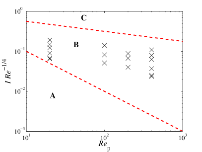
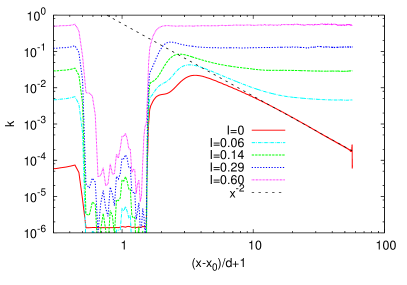
Figure 12: Left: representation in the parameter plane $(\mbox{{Re}}_{\mathrm{p}},I\,\mbox{{Re}}^{-1/4})$ of the three regimes for the wake disturbance (see text). The black crosses are the values corresponding to the numerical simulations. Right: turbulent kinetic energy profile along the symmetry axis for $\mbox{{Re}}_{\mathrm{p}}=400$.

These arguments seem to confirm our speculation on the small-scale modifications of the boundary layer by the turbulent fluctuations to cause the increase of the average drag force. However, Merle et al. (2005) showed that the whole range of turbulent scales contribute to the forces on a bubble. It is thus possible that the characteristic scale $\ell$ that we introduced above actually spread over the full inertial range. Confirming its existence would require very-fine numerical measurements that are beyond the scope of the present work.

To complete these results, let us add some comments on the observed behaviour upstream and downstream the particle. The upstream profile does not seem much altered by the turbulent fluctuations whereas the wake looks heavily modified (see Fig. 7 Right). Upstream we find a clear power-law for the dependence of the velocity deficit as a function of the distance to the particle centre. The measured exponent varies from $\approx-2.5$ for $\mbox{{Re}}_{\mathrm{p}}=20$ to $\approx-3$ for $\mbox{{Re}}_{\mathrm{p}}=400$ and seems independent of the turbulent intensity. The gradients in the boundary layer introduced by the turbulent carrier flow are still subdominant in the upstream region and thus do not change the upstream boundary layer on average. On the other side, the downstream profiles change with both the particle Reynolds number and the turbulent intensity. However, we always find a velocity deficit scaling $\propto x^{-1}$ for the large Reynolds number, independently of $I$. Also, as seen in Fig. 12 (Right), we observe a $x^{-2}$ intermediate decay of the turbulent kinetic energy that is absorbed by outter turbulence when $I$ increases. We do not observe the $x^{-2}$ law for the velocity deficit reported by Amoura et al. (2010). This law should appear as an intermediate asymptotics (Eames et al., 2011) that we might not resolve.

5 Conclusion

In this article we address the question how turbulent fluctuations in the carrier flow influence the drag and lift forces acting on a towed sphere. We find that the average drag significantly increases compared to what is know for a laminar upstream flow. Also the torque of the particle increases as a function of the turbulent intensity. These increases depend on the ratio of the flow advection time across the particle and the Kolmogorov time scale thus assumed to be a small-scale effect. The fluctuations of the drag force are satisfactorily described by standard drag correlations such as that of Schiller & Naumann (1933). Turbulent fluctuations in the upstream flow increase the frequency and strength of the wake detachment at $Re_{p}=400$. The implications of turbulence on the boundary layer and wake of the particle are also addressed. This work also primarily aimed at validating a new method for integrating the incompressible Navier–Stokes equation with no-slip boundary conditions on the surface of a moving particle. Simulations that were performed with this method in the case of a spherical particle embedded in a laminar upstream flow, show that such a strategy reproduces with a high accuracy known results on the variation of the drag and lift forces as a function of the particle Reynolds number and give a precise handling on the turbulent fluctuations that arise in the wake downstream the sphere.

Such benchmarking will now allow us confidently attacking the physical problems that motivated the development of the code. The first question that is subject to ongoing work concerns the dynamics of neutrally buoyant finite-size particles that are transported by a developed turbulent flow in the case when the diameter of such particles falls inside the turbulent inertial range of length scales. The drag, lift, and the slip velocity associated to such settings are still not well defined because of the fluctuating nature of the fluid surrounding environment. This situation still requires an important modelling effort. Today’s models usually rely on applying to turbulent situations formula that are known only for upstream laminar flows, as e.g. Schiller & Naumann (1933). Finite-size models can now be improved with the help of the present results. This work will also give new insights for understanding how the fluid velocity statistical properties are modified by the presence of the particle. Preliminary results on a moving particle confirm that a turbulent boundary layer develops around the particle and that its thickness is comparable to the particle size.

Another important open question that is worth mentioning here relates to possible improvements of the order of the method that is presented here. As we have seen, the error of the proposed method is of the order of $\Delta x^{3/2}$. To go beyond this first order, a natural idea is to make use of the variational formulation that is described in Sec. 2 and which consists in expressing the penalty force as a solution to a minimisation problem. To avoid Gibbs oscillations that, as we showed, are responsible for the observed error, it could be envisaged to relax such minimality to the surface instead of the full particle volume, allowing for instance the fluid flow to develop inside the particle, without affecting the no-slip boundary condition. Such ideas lead to new difficulties related to the non-locality of pressure and which still need to be cautiously worked out.

Acknowledgements

This work benefited from fruitful discussions with J. Dreher. Part of this research was supported by the French Agence Nationale de la Recherche under grant No. BLAN07-1_192604. The research leading to these results has received funding from the European Research Council under the European Community’s Seventh Framework Program (FP7/2007-2013, Grant Agreement no. 240579). Access to the IBM BlueGene/P computer JUGENE at the FZ Jülich was made available through project HBO22. Part of the computations were performed on the “mésocentre de calcul SIGAMM” and using HPC resources from GENCI-IDRIS (Grant 2009-i2010026174).

References

- Amoura et al. (2010) Amoura, Zouhir, Roig, Veronique, Risso, Frederic & Billet, Anne-Marie 2010 Attenuation of the wake of a sphere in an intense incident turbulence with large length scales. Phys. Fluids 22, 055105.
- Anderson & Uhlherr (1977) Anderson & Uhlherr 1977 The influence of stream turbulence on the drag of freely endtrained spheres. In 6th Australasian Hydraulics and Fluid Mechanics Conference Adelaide, Australia, 5-9 December 1977, pp. 541–545.
- Angot et al. (1999) Angot, P., Bruneau, C.H. & Fabrie, P. 1999 A penalization method to take into account obstacles in incompressible viscous flows. Numerische Mathematik 81 (4), 497–520.
- Bagchi & Balachandar (2002) Bagchi, P. & Balachandar, S. 2002 Effect of free rotation on the motion of a solid sphere in linear shear flow at moderate Re. Phys. Fluids 14, 2719–2737.
- Bagchi & Balachandar (2003) Bagchi, P. & Balachandar, S. 2003 Effect of turbulence on the drag and lift of a particle. Phys. Fluids 15 (11), 3496.
- Bagchi & Balachandar (2004) Bagchi, P. & Balachandar, S. 2004 Response of the wake of an isolated particle to an isotropic turbulent flow. J. Fluid Mech. 518, 95–123.
- Balachandar & Eaton (2010) Balachandar, S. & Eaton, John K. 2010 Turbulent Dispersed Multiphase Flow. Annual Review of Fluid Mechanics 42 (1), 111–133.
- Brown et al. (2001) Brown, D. L., Cortez, R. & Minion, M. L. 2001 Accurate Projection Methods for the Incompressible Navier–Stokes Equations. J. Comp. Phys. 168 (2), 464–499.
- Brucato et al. (1998) Brucato, A, Grisafi, F & Montante, G 1998 Particle drag coefficients in turbulent fluids. Chemical engineering science 53 (18), 3295–3314.
- Burton & Eaton (2005) Burton, T. & Eaton, J. K. 2005 Fully resolved simulations of particle-turbulence interaction. J. Fluid Mech. 545, 67.
- Calzavarini et al. (2009) Calzavarini, E., Volk, R., Bourgoin, M., Leveque, E., Pinton, J.F. & F.Toschi 2009 Acceleration statistics of finite-sized particles in turbulent flow: the role of faxen forces. J. Fluid Mech. 630, 179.
- Calzavarini et al. (2011) Calzavarini, E., Volk, R., Lévêque, E., Pinton, J.F. & F.Toschi 2011 Impact of trailing wake drag on the statistical properties and dynamics of finite-sized particle in turbulence. to appear in Physica D .
- Dandy & Dwyer (1990) Dandy, D.S. & Dwyer, H.A. 1990 A sphere in shear flow at finite Reynolds number: effect of shear on particle lift, drag, and heat transfer. J. Fluid Mech. 216, 381–410.
- Eames et al. (2011) Eames, I., Johnson, P. B., Roig, V. & Risso, F. 2011 Effect of turbulence on the downstream velocity deficit of a rigid sphere. Phys. Fluids 23, 095103.
- Fadlun et al. (2000) Fadlun, E A, Verzicco, R, Orlandi, P & Mohd-Yusof, J 2000 Combined Immersed-Boundary Finite-Difference Methods for Three-Dimensional Complex Flow Simulations. J. Comp. Phys. 60, 35–60.
- Frisch (1995) Frisch, Uriel 1995 Turbulence. Cambridge: Cambridge University Press.
- Goldstein et al. (1993) Goldstein, D., Handler, R. & Sirovich, L. 1993 Modeling a no-slip flow boundary with an external force field. J. of Comp. Phys. 105, 354–366.
- Homann & Bec (2010) Homann, H. & Bec, J. 2010 Finite-size effects in the dynamics of neutrally buoyant particles in turbulent flow. J. Fluid Mech. 651, 81–91.
- Kim & Balachandar (2012) Kim, Jungwoo & Balachandar, S. 2012 Mean and fluctuating components of drag and lift forces on an isolated finite-sized particle in turbulence. Theoretical and Computational Fluid Dynamics 26 (1), 185–204.
- Kolmogorov (1941) Kolmogorov, A. N. 1941 Energy dissipation in locally isotropic turbulence. Dokl. Akad. Nauk SSSR 32, 19–21.
- Kurose & Komori (1999) Kurose, R. & Komori, S. 1999 Drag and lift forces on a rotating sphere in a linear shear flow. J. Fluid Mech. 384, 183–206.
- Le Clair et al. (1970) Le Clair, B. P., Hamielec, A. E. & Pruppacher, H.R. 1970 A Numerical Study of the Drag on a Sphere at Low and Intermediate Reynolds Numbers. Journal of Atmospheric 27, 308–315.
- Lin et al. (1970) Lin, C.J., Peery, J.H. & Showalter, W.R. 1970 Simple shear flow round inertial effects and suspension rheology. J. Fluid Mech. 44, 1–17.
- Luo et al. (2010) Luo, Kun, Wang, Zeli & Fan, Jianren 2010 Response of force behaviors of a spherical particle to an oscillating flow. Phys. Lett. A 374 (30), 3046 – 3052.
- Merle et al. (2005) Merle, Axel, Legendre, Dominique & Magnaudet, Jacques 2005 Forces on a high-Reynolds-number spherical bubble in a turbulent flow. J. Fluid Mech. 532, 53–62.
- Mohd-Yusof (1997) Mohd-Yusof, J. 1997 Combined immersed boundary/b-spline methods for simulations of flow in complex geometries. Center for Turbulence Research – Annual Research Briefs pp. 317–327.
- Naso & Prosperetti (2010) Naso, A. & Prosperetti, A. 2010 The interaction between a solid particle and a turbulent flow. New Journal of Physics 12 (3), 033040.
- Pasquetti et al. (2008) Pasquetti, R., Bwemba, R. & Cousin, L. 2008 A pseudo-penalization method for high reynolds number unsteady flows. Appl. Numer. Math. 58 (7), 946–954.
- de Pater & Lissauer (2001) de Pater, I. & Lissauer, J. 2001 Planetary Science. Cambridge: Cambridge University Press.
- Patterson & Orszag (1971) Patterson, G.S. & Orszag, S.A. 1971 Spectral calculation of isotropic turbulence: efficient removal of aliasing interaction. Phys. Fluids 14, 2538–2541.
- Peskin (1977) Peskin, C.S. 1977 Numerical analysis of blood flow in the heart. J. Comp. Phys. 25, 220–252.
- Pope (2000) Pope, S.B. 2000 Turbulent flows, 1st edn. Cambridge: Cambridge University Press.
- Prosperetti & Oguz (2001) Prosperetti, A. & Oguz, H.N. 2001 Physalis: A New o(N) Method for the Numerical Simulation of Disperse Systems: Potential Flow of Spheres. J. Comp. Phys. 167 (1), 196–216.
- Qureshi et al. (2007) Qureshi, Nauman M, Bourgoin, Mickaël, Baudet, Christophe, Cartellier, Alain & Gagne, Yves 2007 Turbulent transport of material particles: an experimental study of finite size effects. Physical Review Letters 99 (18), 184502.
- Schiller & Naumann (1933) Schiller, L. & Naumann, A. 1933 über die grundlegenden berechnungen bei der schwerkraftaufbereitung. Verein Deutscher Ingenieure 77, 318.
- Schlichting (1979) Schlichting, H. 1979 Boundary-Layer Theory. New York, United States: McGraw-Hill.
- Seinfeld & Pandis (1998) Seinfeld, J. H. & Pandis, S. N. 1998 From Air Pollution to Climate Change. John Wiley and Sons.
- Shaw (2003) Shaw, Raymond A. 2003 Particle-Turbulence Interactions in Atmospheric Clouds. Annual Review of Fluid Mechanics 35 (1), 183–227.
- Shu & Osher (1988) Shu, C. & Osher, S. 1988 Efficient implementation of essentially non-oscillatory shock-capturing schemes. J. Comput. Phys. 77, 439–471.
- Taira & Colonius (2007) Taira, K. & Colonius, T. 2007 The immersed boundary method: A projection approach. J. Comp. Phys. 225 (2), 2118–2137.
- Uberoi & Freymuth (1970) Uberoi, M.S. & Freymuth, P. 1970 Turbulent energy balance and spectra of the axisymmetric wake. Phys. Fluids 13, 2205.
- Uhlmann (2005) Uhlmann, M 2005 An immersed boundary method with direct forcing for the simulation of particulate flows. J. Comp. Phys. 209 (2), 448–476.
- Volk et al. (2010) Volk, R., Calzavarini, E., Leveque, E. & Pinton, J.-F. 2010 Dynamics of inertial particles in a turbulent von Karman flow. accepted for publication in J. Fluid Mech. p. 10.
- Warnica et al. (1995) Warnica, W.D., Renksizbulut, M. & Strong, A.B. 1995 Drag coefficients of spherical liquid droplets Part 2: Turbulent gaseous fields. Experiments in Fluids 18 (4), 265–276.
- Wu & Faeth (1994) Wu, J.-S. & Faeth, G. M. 1994 Sphere wakes at moderate Reynolds numbers in a turbulent environment. AIAA Journal 32 (3), 535–541.
- Xu & Bodenschatz (2008) Xu, H. & Bodenschatz, E. 2008 Motion of inertial particles with size larger than Kolmogorov scale in turbulent flows. Physica D: Nonlinear Phenomena 237 (14-17), 2095–2100.
- Yeo et al. (2010) Yeo, K., Dong, S., Climent, E. & Maxey, M.R. 2010 Modulation of homogeneous turbulence seeded with finite size bubbles or particles. International Journal of Multiphase Flow 36 (3), 221–233.