Direct calculation of the attempt frequency of magnetic structures using the finite element method

Abstract

A numerical implementation of the transition state theory (TST) is presented which can be used to calculate the attempt frequency $f_{0}$ of arbitrary shaped magnetic nanostructures. The micromagnetic equations are discretized using the finite element method. The climbing image nudged elastic band method is used to calculate the saddle point configuration, which is required for the calculation of $f_{0}$. Excellent agreement of the implemented numerical model and analytical solutions is obtained for single domain particles. The developed method is applied to compare $f_{0}$ for single phase and graded media grains of advanced recording media. $f_{0}$ is predicted to be comparable if the maximum anisotropy is the same in these two media types.

[1] Institute of Solid State Physics, Vienna University of Technology, Vienna 1040, Austria

[2] St. Poelten University of Applied Sciences, St. Poelten 3130, Austria

[3] School of Physics, M013, University of Western Australia, 35 Stirling Hwy, Crawley Western Australia 6009, Australia

[4] UCD School of Physics, University College Dublin, Belfield, Dublin 4, Ireland

1 Introduction

A detailed knowledge of the thermal stability is of utmost importance for magnetic nanostructures for various applications ranging from hard disc media, MRAM devices to permanent magnets. A well established tool which originated in chemical rate theory for determining the thermal stability relies on the transition state theory (TST). In the TST the thermal stability of a minimum energy state $M_{1}$ is determined by the application of the Arrhenius-Neel law, $\tau=\frac{1}{f_{0}}e^{\frac{\Delta E}{k_{B}T}}$, where the energy barrier $\Delta E$ separates the minimum energy state $M_{1}$ and the saddle point configuration $S_{1}$. The attempt frequency $f_{0}$ limits the probability for reversal.

The thermal stability, which requires the calculation of the energy barrier and the attempt frequency was first calculated for single domain particles in the intermediate to high damping limit (IHD) for an external field applied exactly parallel to the easy axis[2]. For systems where the symmetry is broken either by an oblique external field or by an additional anisotropy various works are published giving analytical formulas for the attempt frequency for different damping limits. For the IHD limit formulas for the thermal stability can be found in Ref [19, 12, 3, 4]. For the limit of very low damping a formula for the thermal stability was derived by Smith et al [19]. In order to extend the calculation of the damping limit to all values of the damping constant Coffey et al. [5]and Déjardin et al. [6]have shown that the Mel’nikov-Meshkov formalism can be applied to magnetic systems. Analytical formulas for the intermediate damping regime are given by Garanin et al [8].

All the previous mentioned work were restricted to reversal via homogeneous rotation. Inhomogenous states were treated by Braun who calculated the thermally activated reversal in elongated particles [1]. Besides analytical formulas for the attempt frequency he found that the thermal stability depends on the domain wall energy in these elongated particles.

The approach of Braun was extended to soft/hard bilayers, where the saddle point configuration can be described by a domain wall at the soft/hard interface by Loxley et al [16].

The paper is structured as follows. In section II details of the implementation of the transition state theory in the finite element package FEMME [22]is given. The implementation method is compared to analytical solutions in section III. An improved method for the calculation of $f_{0}$ is presented in section IV. Summary and discussion are given in section V.

2 Numerical Calculation of the Attempt Frequency

The numerical implementation is based on Kramers transition state theory [13], which Langer transposed and expanded to multidimensional systems in 1967 [14]. According to Langers approach the attempt frequency determines the probability current for the configuration distribution on the energy surface around the saddle point.

The following steps are required in order to calculate the attempt frequency by the means of the transition state theory:

1. The configuration of the system at the minimum and at the saddle point given as the values of all degrees of freedom.

2. The value and curvature of the Gibbs free energy surface at the minimum and at the saddle point with respect to appropriate canonical variables.

3. The systems’ equation of motion in canonical variables along the energy surface to describe the dynamics around the saddle point.

Knowledge of the above properties allows one to calculate the attempt frequency. This can be written as:

$$f_{0} = \frac{\lambda_{+}}{2\pi}\Omega_{0}$$ (1)

2.1 Dynamical factor $\lambda_{+}$ from the Landau-Lifshitz-Gilbert equation

The dynamical factor $\lambda_{+}$ is obtained by solving the noiseless linearized equation of motion. In micromagnetics the equation of motion can be written in the form of the Landau-Lifshitz-Gilbert equation as,

$$\frac{\partial}{\partial t}\vec{J}=-\frac{\gamma}{1+\alpha^{2}}\vec{J}\times\vec{H_{eff}}-\frac{\alpha}{1+\alpha^{2}}\frac{\gamma}{J_{S}}\vec{J}\times(\vec{J}\times\vec{H_{eff}})$$ (2)

where the magnetic polarization $\vec{J}$ and the effective $\vec{H_{eff}}$ field are continuous functions of space. In the following, we discretize the continuous equation of motion using the finite element method using the box scheme [22, 10]. We can write for the effective field on the node point $i$,

$$H_{eff,i}\approx-\frac{1}{V_{i}}\left(\frac{\partial E}{\partial J_{i}}\right)$$ (3)

with $V_{i}$ being the corresponding volume of spin $i$ and $E$ being the Total Gibbs energy. The structure of the Landau-Lifshitz-Gilbert equation leads to a constant length of the magnetic polarization $\left|\vec{J}\right|=J_{s}$ . As a consequence the number of independent equation is $2N$, where $N$ is the number of spins. In order to apply the theory developed by Langer the system has to be expressed with its canonical variables [14]. For a system with $N$-spins the canonical variables on node point $i$ are given by [9, 17],

$$\begin{array}[]{c}p_{i}=V_{i}J_{s}\cos(\theta_{i})\\ q_{i}=\phi_{i}\end{array}$$ (4)

where the polar angle angle $\phi_{i}$ and azimuthal angle $\theta_{i}$ are defined as,

$$\overrightarrow{J_{i}}=J_{s}\left(\sin\theta_{i}\cos\phi_{i},\sin\theta_{i}\sin\phi_{i},\cos\theta_{i}\right)$$ (5)

The Landau-Lifshitz-Gilbert equation for spin $i$ in canonical variables reads,

$$\begin{pmatrix}\frac{\partial p_{i}}{\partial t}\\ \frac{\partial q_{i}}{\partial t}\end{pmatrix}=-\frac{\gamma}{J_{s}V_{i}(1+\alpha^{2})}\frac{1}{sin\theta_{i}}\begin{pmatrix}-J_{s}V_{i}\alpha sin^{2}\theta_{i}\frac{\partial E}{\partial\theta_{i}}-J_{s}V_{i}sin\theta_{i}\frac{\partial E}{\partial\phi_{i}}\\ -\frac{\partial E}{\partial\theta_{i}}+\frac{\alpha}{sin\theta_{i}}\frac{\partial E}{\partial\phi_{i}}\end{pmatrix}$$ (6)

Let us denote $\eta_{2i-1}=p_{i}$ and $\eta_{2i}=q_{i}$. We can write the equation of motion in the form,

$$\frac{\partial\eta_{2i-1}}{\partial t}=\frac{\partial p_{i}}{\partial t}=:f_{2i-1}(\eta_{1},...,\eta_{2N})$$ (7)

$$\frac{\partial\eta_{2i}}{\partial t}=\frac{\partial q_{i}}{\partial t}==:f_{2i}(\eta_{1},...,\eta_{2N})$$ (8)

Transition state theory considers the linear dynamics around the saddle point. Linearizing the right hand side around the saddle point, we obtain:

$$\begin{pmatrix}\frac{\partial\eta_{1}}{\partial t}\\ \vdots\\ \frac{\partial\eta_{2N}}{\partial t}\end{pmatrix}\approx\left.\begin{pmatrix}f_{1}\\ \vdots\\ f_{2N}\end{pmatrix}\right|_{sp}+\left.\begin{pmatrix}\frac{\partial f_{1}}{\partial\eta_{1}}&\ldots&\frac{\partial f_{1}}{\partial\eta_{2N}}\\ \vdots&\ddots&\vdots\\ \frac{\partial f_{2N}}{\partial\eta_{1}}&\ldots&\frac{\partial f_{2N}}{\partial\eta_{2N}}\end{pmatrix}\right|_{sp}\begin{pmatrix}\eta_{1}-\eta_{sp,1}\\ \vdots\\ \eta_{2N}-\eta_{sp,2N}\end{pmatrix}$$ (9)

The first derivatives of the energy with respect to the spin components at the saddle point is zero, thus the first term on the right hand side is zero as well. The second term we define as $H_{dyn}$:

$$H_{dyn}:=\left.\begin{pmatrix}\frac{\partial f_{1}}{\partial\eta_{1}}&\ldots&\frac{\partial f_{1}}{\partial\eta_{2N}}\\ \vdots&\ddots&\vdots\\ \frac{\partial f_{2N}}{\partial\eta_{1}}&\ldots&\frac{\partial f_{2N}}{\partial\eta_{2N}}\end{pmatrix}\right|_{sp}$$ (10)

The last term we define as vector $\nu_{k}=\eta_{k}-\eta_{sp,k}$. The time derivative of $\vec{\nu}$ equals the left hand side of Equation 9. So Eq. 9 can be written as:

$$\frac{\partial\vec{\nu}}{\partial t}\approx H_{dyn}\vec{\nu}$$ (11)

This is a linear system of differential equations which has 2N eigenvalues $\lambda_{k}$ with corresponding eigenvectors $\vec{\nu_{k}}^{0}$. The solutions are of the form:

$$\vec{\nu_{k}}=\vec{\nu_{k}}^{0}e^{\lambda_{k}t}$$ (12)

With the exception of one eigenvalue, all other eigenvalues of the matrix $H_{dyn}$ at the saddle point are negative. This single positive eigenvalue is the $\lambda_{+}$ that we need for the calculation of the attempt frequency.

For the numerical calculation of $H_{dyn}$, the function $f=f_{i}$ has to be derived with respect to the coordinate $x=\eta_{i}$. This was calculated numerically using finite differences and a seven point stencil method.

$$f^{\prime}(x)\approx\frac{-f(x-3h)+9f(x-2h)-45f(x-h)+45f(x+h)-9f(x+2h)+f(x+3h)}{60h}$$ (13)

The step size used in the numerical results was $h=0.005$

2.2 Statistical factor $\Omega_{0}$ from the Hessian matrix

The statistical factor $\Omega_{0}$ relates the curvature of the total Gibbs energy with respect to the canonical variables at the saddle point and at the minimum. The curvature is obtained by calculating the second derivative of the energy,

$$H:=\left(\begin{array}[]{ccc}\frac{\partial h_{1}}{\partial\eta_{1}}&\cdots&\frac{\partial h_{1}}{\partial\eta_{2N-2}}\\ \vdots&\ddots&\vdots\\ \frac{\partial h_{2N-2}}{\partial\eta_{1}}&\cdots&\frac{\partial h_{2N-2}}{\partial\eta_{2N-2}}\end{array}\right)$$ (17)

$$=\left(\begin{array}[]{ccc}\frac{\partial^{2}E}{\partial\eta_{1}\partial\eta_{1}}&\cdots&\frac{\partial^{2}E}{\partial\eta_{2N-2}\partial\eta_{1}}\\ \vdots&\ddots&\vdots\\ \frac{\partial^{2}E}{\partial\eta_{1}\partial\eta_{2N-2}}&\cdots&\frac{\partial^{2}E}{\partial\eta_{2N-2}\partial\eta_{2N-2}}\end{array}\right)$$

$\Omega_{0}$ is the square root of the ratios of the determinants of the Hessian matrices at the minimum and the saddle point:

$$\Omega_{0} = \sqrt{\frac{\textup{det}\,H_{min}}{|\textup{det}\,H_{sp}|}}$$ (18)

It is important to note, that the theory of transitions as developed by Langer is only valid for canonical variables. Suppose that instead of the canonical variables$\left(p_{i},q_{i}\right)$, the polar angles $\left(\theta_{i},\phi_{i}\right)$ are used to describe the system (see e.g. Ref [18]) and its derivatives $\frac{\partial^{2}E}{\partial\theta_{i}\partial\phi_{i}}$. Then the obtained $f_{0}$ is correct only if the magnetic state at the minimum and the saddle point fulfills $\theta_{i}=\pi/2$ for all spins. This prerequisite is, for example, fulfilled for a single domain particle having the easy axis pointing along the x-axis and an external field applied along the y-axis as in Ref [18]. The same argument applies for the calculation of $\lambda_{+}$.

For the numerical calculation of the derivative the same finite difference scheme was used as described in the previous section.

2.3 Climbing Image Nudged Elastic Band Method

The calculation of the statistical prefactor $\Omega_{0}$ and the calculation of $\lambda_{+}$ require knowledge of the saddle point configuration. A very accurate calculation of the saddle point configuration is essential for the calculation of the attempt frequency. The nudged elastic band method was used in order to calculate the saddle point configuration [20, 7]. It was found that the accuracy of the nudged elastic band method is not sufficiently high in order to calculate reliably the attempt frequency. In order to improve the accuracy of the saddle point determination, a climbing image elastic band method was implemented [11].

3 Validation of the method

3.1 Small magnetic cube

In order to test the numerical calculation of the attempt frequency, we compared the analytically obtained attempt frequency for a single domain particle with uniaxial anisotropy to the numerically obtained one. For the numerical model the following parameters were used: damping constant $\alpha=1$ , anisotropy constant $K_{1}=1.0MJ/m^{3}$ , magnetic saturation polarization $J_{s}=0.5T$ and exchange constant $A=10pJ/m$. The model size is 0.6 x 0.6 x 0.6 nm³. 12 finite elements were used to discretize the cube. The easy axis of the cube was assumed to be parallel to the x-axis. The external field was applied parallel to the y-axis. Results were compared to those obtained using the analytically derived expression for the attempt frequency given in Ref. [18].

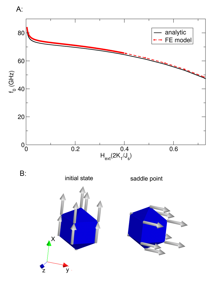
In Fig. 1 (B) two magnetization states of the homogeneous cube are shown: on the left the initial state is depicted, with magnetization pointing close to the the easy axis. On the right the magnetization is shown at the saddle point of the energy, where the magnetization is perpendicular to the easy axis. The magnetization vectors of all nodes are shown. Due to the small structure size, all spin vectors are almost perfectly parallel to each other, indicating that we should expect a good agreement with the analytic result.

In order to compare the numerical results directly with the analytical results, the attempt frequency is plotted as a function of the external field strength as shown in 1 (A) . The simulations agree very well with the analytical solution. It should be noted, that both the analytical solution and the numerical simulation are not valid for zero external field, since the expressions for field lowered symmetry are used. As a consequence the spike-like increase at zero external field is an artifact and has no physical meaning.

3.2 Elongated particle

As a second example we calculate the attempt frequency of an elongated particle. The simulated geometry of the elongated grain is: length 25 nm, width 1.6 x 1.6 nm. This shape is similar to the magnetic grains used as the recording media in modern hard disks, only slimmer (die lateral dimension of a grain of a hard disc is about 6 x 6 nm). According to the analytical theory of Ref. [16]the cross section area does not influence the attempt frequency. Hence, in order to save computational time we model the grain of a recording media with a smaller cross section but we can expect that the results can be used for realistic grains.

The following parameters were used for the graded media grain example: damping constant $\alpha=0.2$ , anisotropy constant increasing quadratically from zero to $K_{1}=3.6MJ/m^{3}$ , magnetic saturation polarization $J_{s}=0.5T$ and exchange constant $A=10pJ/m$. The material parameters are the same as in Ref [21].

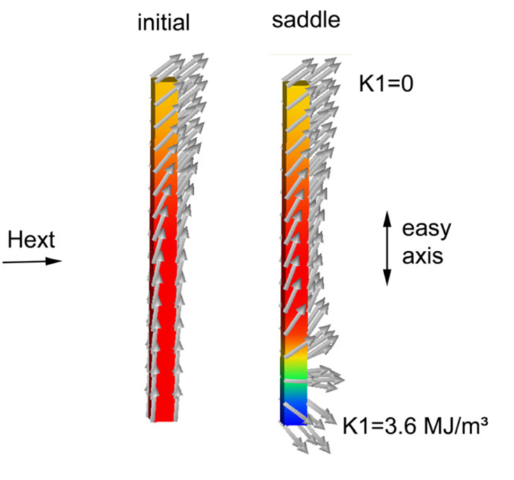
Fig. 2 shows the simulated grain with quadratically increasing $K_{1}$ . The directions of the easy-axis and the applied perpendicular external magnetic field are shown. The magnetic state at the minimum of the energy is shown on the left side of the figure, and the saddle point is shown on the right side.

As in the previous section the attempt frequency was calculated as a function of a perpendicular applied field. In order to verify reliability, the simulations were repeated with different finite element meshes.

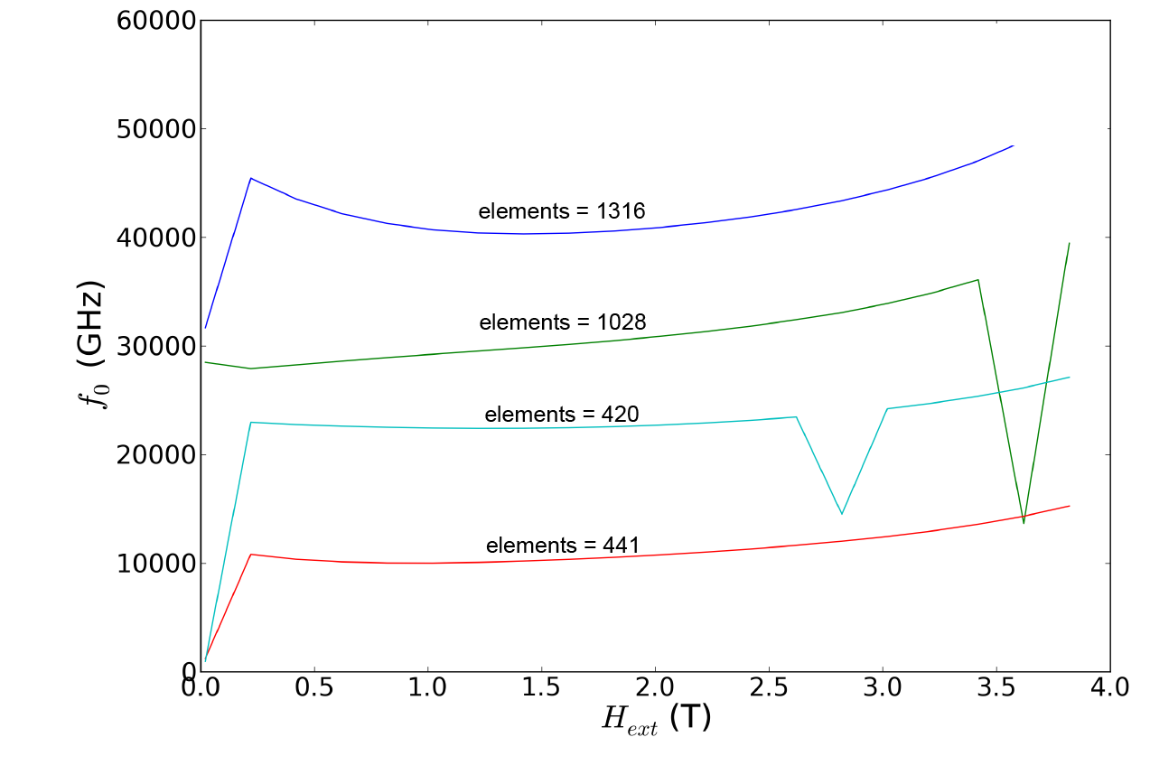
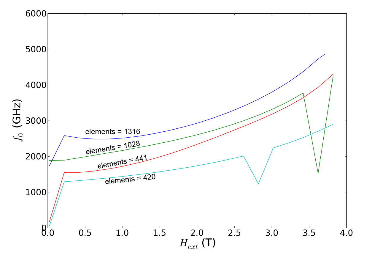
Fig. 3 shows the attempt frequency of four different finite element meshes, with different numbers of volume elements. As can be seen, the results of the attempt frequency do not converge to a single value as the finite element mesh size is decreased. Furthermore the obtained value of the attempt frequency is one order of magnitude larger than the value reported in Ref [21]. The reason for these discrepancies are discussed in the next section.

4 Improved method using analytical fits

The reason for the numerical errors of the attempt frequency can be found in the calculation of $\Omega_{0}$, which consists of (the square root of) a ratio of determinants as given by Eq.18. The calculation of the determinant of the symmetric matrix $H$ equals the product of all its eigenvalues $\lambda_{1}$, . . . , $\lambda_{2N}$, where $N$ is the number of finite element node points.

Hence, we can write $\Omega_{0}$ in the form:

$$\Omega_{0} =\sqrt{\frac{\prod\lambda_{min_{i}}}{|\prod\lambda_{sp_{i}}|}}=\sqrt{\left|\frac{\prod\lambda_{min_{i}}}{\prod\lambda_{sp_{i}}}\right|}$$

All eigenvalues of $H_{min}$ at the minimum are positive. At the saddle point there is only one negative eigenvalue. The number of eigenvalues increases with increasing number of finite elements. Hence, small numerical errors in the calculation of the eigenvalues multiply together to form a considerable total error.

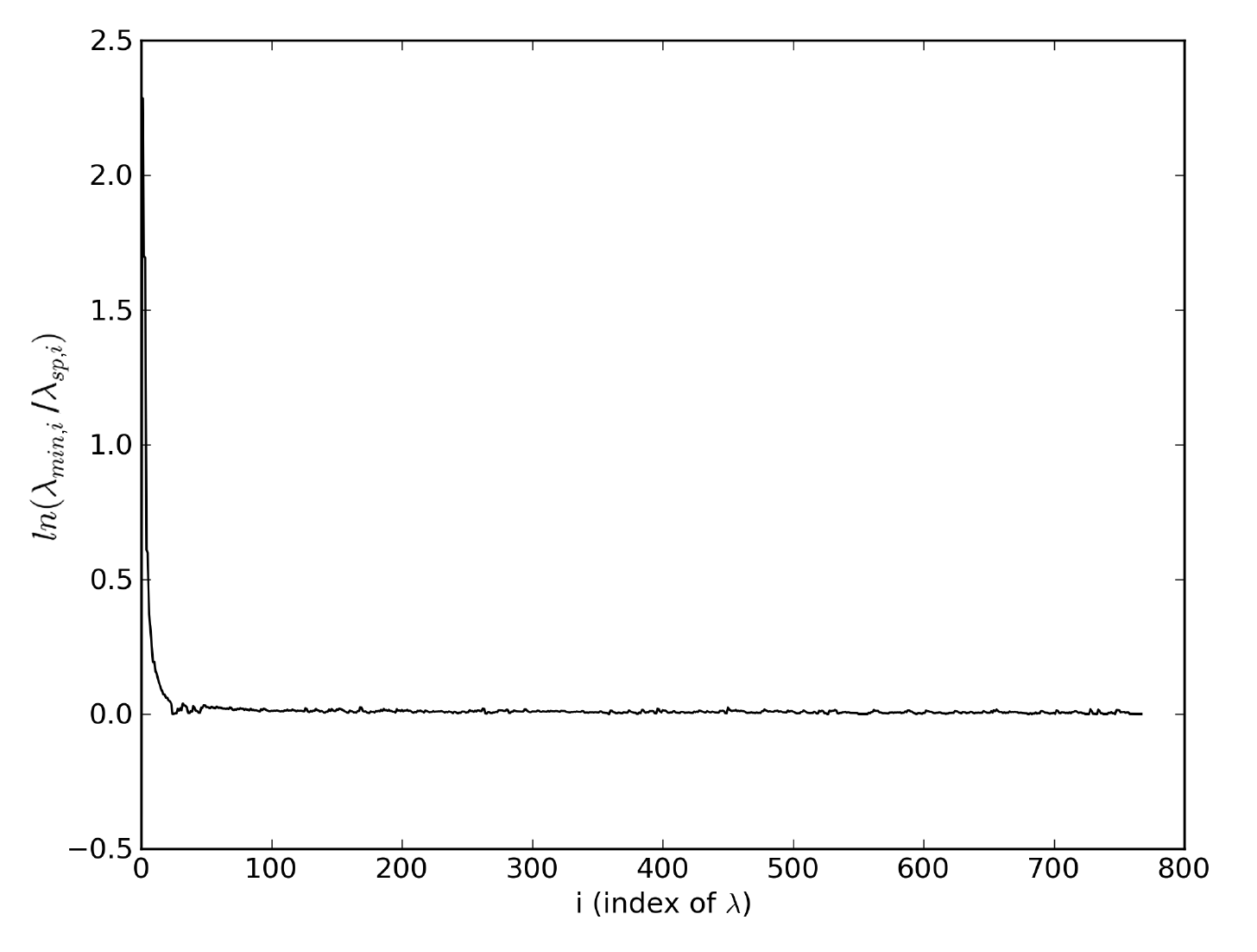
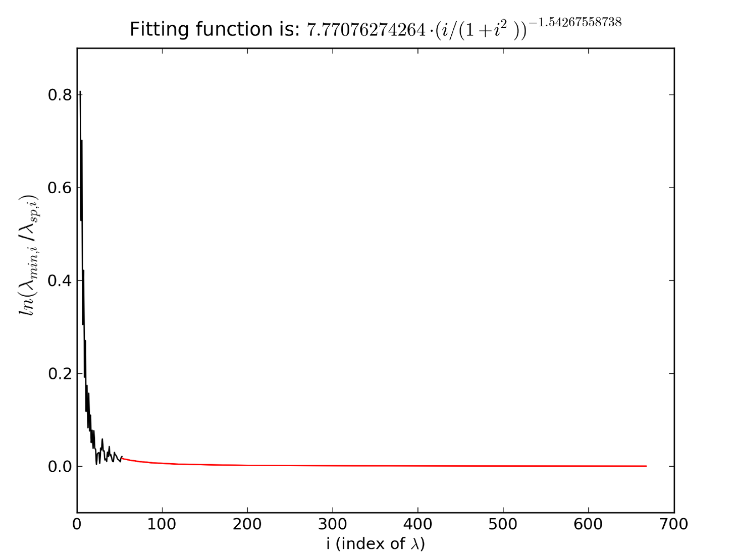
Fig. 4 shows the ratio of the eigenvalues. The x-axis represents the index $i$ of the eigenvalues, and the y-axis represents the natural logarithm of the ratios of eigenvalues, $\lambda_{min,i}/\lambda_{sp,i}$. In Fig. 4 the eigenvalues are sorted according to modulus, where the eigenvalue with the index $i=1$ has the smallest modulus and $i=2N$ is the eigenvalue with the largest modulus. As shown in Fig. 4 only ratios of eigenvalues with small i are not close to or equal to 1. All the ratios of the eigenvalue with $i>>100$ are very close to one, which results in $\ln(\lambda_{min,i}/\lambda_{sp,i})\thickapprox 0$ for $i>>100$.

The numerical evidence in Fig. 4 illustrate the insensitivity of the saddle point to the majority of eigenmodes, and the thermal significance of modes with the smallest eigenvalues. As noted in Ref [15], a domain wall pinned at an interface supports a broad range of travelling spin waves that are essentially unperturbed by the wall structure, and a set of modes localized to the domain wall. The modes localized to the wall have the smallest eigenvalues, and represent the most relevant fluctuations for thermal depinning of the wall.

Braun has shown that for elongated particles, the logarithm of the ratio of eigenvalues scales with $\frac{i}{1+i^{2}}$ (see formula (4.12) of Ref. [1]).

In order to reduce the numerical error which is introduced by the higher order eigenfrequency, we fit the values of $\ln(\lambda_{min,i}/\lambda_{sp,i})$ to the following function,

$$f(i)=a\cdot\left(\frac{i}{1+i^{2}}\right)^{b}$$ (19)

, where $a$ and $b$ are parameters determined by a mean square fit to the numerical data for $5<i<60$. In Fig. 5 the black line represents the ratios of eigenvalues, calculated by the numerical simulation, and the red line is the fitted function, which values of parameters $a$ and $b$ are given in the inset. The calculation of $\Omega_{0}$ is done by calculating $\Omega_{0}=\sqrt{\left|\prod_{i=0}^{c}{\frac{\lambda_{min_{i}}}{\lambda_{sp_{i}}}}\cdot\prod_{i=c+1}^{N}{e^{fit(i)}}\right|}$. We found for a wide range of c ($10<c<100$) that the value of $\Omega_{0}$ is not significantly influenced by the actual choosen value of the paramter c.

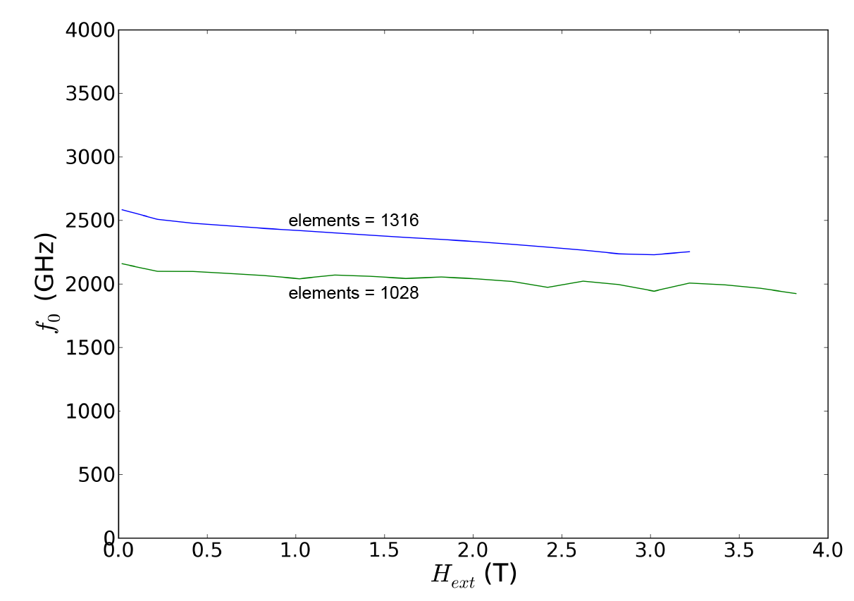
The calculation of the attempt frequency of the graded media grain is repeated with the improved method using the fit function. Fig. 6 shows that the mesh dependency of the results is decreased by this method. If the value of the attempt frequency is extrapolated for an external field approaching zero we can estimate the attempt frequency to be in the order of $f_{0}\sim 1850GHz\pm 650GHz$. Comparing this estimate of the attempt frequency with the estimate of the attempt frequency obtained by Langevin dynamic simulations (In Ref. [21] for the same system a value of $f_{0}\sim 1638GHz\pm 46GHz$ is estimated), despite the various assumptions which are used in both methods, a considerable good agreement can be found.

From an application point of view it is interesting to compare the attempt frequency of a grain with graded anisotropy to the attempt frequency of grain for which anisotropy is uniform throughout. Fig. 7 shows the attempt frequency of a single phase grain, where all the material parameters are the same as for the graded media grain of Fig. 6 except that the anisotropy is a constant $K_{1}\sim 3.6$MJ/m³. This value equals the maximum anisotropy constant of the graded media grain of the previous results.

5 Results and discussion

A numerical implementation of the transition state theory was described with application to two example problems: reversal of a single phase and graded media magnetic grains. The implementation makes use of the micromagnetic package FEMME. This method allows for the calculation of the long term thermal stability of magnetic nanostructures without any free parameters. The input parameters of the model are the exchange constant, the anisotropy constant the spontaneous saturation magnetization, the damping constant and the geometry of the magnet. The advantage of the presented method over Langevin-dynamic simulation is that the thermal stability of large magnetic nanostructures can be calculated. Furthermore Langevin-dynamic simulations are restricted to time scales of several nano-seconds due to computational effort.

In previous work it was shown that so called exchange spring media exhibit superior writeability as compared to single phase media, without lowering the energy barrier [suess_multilayer_2006]. The energy barrier was assumed to determine the thermal stability. In this paper we show the exact relation of the energy barrier and the thermal stability by calculating the attempt frequency. In the present paper we show that the attempt frequency and energy barrier aare comparable for a single phase media and a graded media grain with single phase grain anisotropy is the same as the maximum anisotropy in the graded media grain. Hence, it was shown that these two media types indeed have very similar thermal stabilities but the coercive field for the graded media grain is about a factor of seven smaller than the single phase grain.

The financial support of the FWF projects P20306-N16 and SFB ViCoM (F4112-N13) is acknowledged.

Figure 1: (color online) (A) the numerically calculated attempt frequency of a small magnetic particle is compared with the analytical result as a function of the external applied field (H field applied along y-axis, easy axis parallel to x-axis). (B) The magnetic state at the minimum (left) and at the saddle point (right) is shown.

Figure 2: (color online) model of the graded media grain which is soft magnetic at the top and hard magnetic at the bottom. (left) energy minimum state (right) saddle point configuration.

Figure 3: (color online) The attempt frequency as a function of the external field strength is shown for a graded media grain. The external field is applied perpendicular to the easy axis. The results are shown as a function of the number of finite elements.

Figure 4: Logarithmic ratios of eigenvalues as a function of the eigenvalue index i. (number of finite elements= 1316 , H_ext is 0.02 T.)

Figure 5: Contributions to calculation of $\Omega_{0}$: up to index 50 the original data is taken (black line), and from index 50 onwards the values of the fitting function are used (red line).

Figure 6: Same as Fig. 3 except that a fitting function from eigenvalue index 30 onwards is used for the calculation of $\Omega_{0}$.

Figure 7: Attempt frequency of a single phase media calculated for two different mesh sizes (For the calculation of $\Omega_{0}$ a fitting function from eigenvalue index 30 onwards is used).

References

- [1] Hans-Benjamin Braun. Statistical mechanics of nonuniform magnetization reversal. Physical Review B, 50(22):16501, December 1994.
- [2] W.F. Brown. Thermal fluctuations of a single-domain particle. Physical Review, 130(5):1677–1686, 1963.
- [3] W.T. Coffey, D.S.F. Crothers, J.L. Dormann, L.J. Geoghegan, and E.C. Kennedy. Effect of an oblique magnetic field on the superparamagnetic relaxation time. II. influence of the gyromagnetic term. Physical Review B - Condensed Matter and Materials Physics, 58(6):3249–3266, 1998.
- [4] W.T. Coffey, D.S.F. Crothers, J.L. Dormann, Yu.P. Kalmykov, E.C. Kennedy, and W. Wernsdorfer. Thermally activated relaxation time of a single domain ferromagnetic particle subjected to a uniform field at an oblique angle to the easy axis: Comparison with experimental observations. Physical Review Letters, 80(25):5655–5658, 1998.
- [5] W.T. Coffey, D.A. Garanin, and D.J. McCarthy. Crossover formulas in the Kramers theory of thermally activated escape rates - Application to spin systems, volume 117. 2001.
- [6] P.M. Déjardin, D.S.F. Crothers, W.T. Coffey, and D.J. McCarthy. Interpolation formula between very low and intermediate-to-high damping kramers escape rates for single-domain ferromagnetic particles. Physical Review E - Statistical, Nonlinear, and Soft Matter Physics, 63(2 I):0211021–02110212, 2001.
- [7] R. Dittrich, T. Schrefl, D. Suess, W. Scholz, H. Forster, and J. Fidler. A path method for finding energy barriers and minimum energy paths in complex micromagnetic systems. Journal of Magnetism and Magnetic Materials, 250, 2002.
- [8] D. A. Garanin, E. C. Kennedy, D. S. F. Crothers, and W. T. Coffey. Thermally activated escape rates of uniaxial spin systems with transverse field: Uniaxial crossovers. Physical Review E, 60(6):6499, December 1999.
- [9] J. L. García-Palacios and D. A. Garanin. Nonlinear response of superparamagnets with finite damping: An analytical approach. Physical Review B, 70(6):064415, 2004.
- [10] C. W Gardiner. Handbook of stochastic methods. Springer Berlin, 1985.
- [11] Graeme Henkelman, Blas P. Uberuaga, and Hannes Jo?nsson. A climbing image nudged elastic band method for finding saddle points and minimum energy paths. The Journal of Chemical Physics, 113(22):9901, 2000.
- [12] William Fuller Brown Jr. Thermal fluctuations of fine ferromagnetic particles. IEEE Transactions on Magnetics, MAG-15(5):1196–1208, 1979.
- [13] H.A. Kramers. Brownian motion in a field of force and the diffusion model of chemical reactions. Physica, 7(4):284–304, 1940.
- [14] J.S. Langer and L.A. Turski. Hydrodynamic model of the condensation of a vapor near its critical point. Physical Review A, 8(6):3230–3243, 1973.
- [15] K. L. Livesey, D. C. Crew, and R. L. Stamps. Spin wave valve in an exchange spring bilayer. Physical Review B, 73(18):184432, May 2006.
- [16] P.N. Loxley and R.L. Stamps. Theory for nucleation at an interface and magnetization reversal of a two-layer nanowire. Physical Review B - Condensed Matter and Materials Physics, 73(2):1–14, 2006.
- [17] E. Magyari, H. Thomas, R. Weber, C. Kaufman, and G. Müller. Integrable and nonintegrable classical spin clusters - integrability criteria and analytic structure of invariants. Zeitschrift für Physik B Condensed Matter, 65(3):363–374, 1987.
- [18] J. Schratzberger, J. Lee, M. Fuger, J. Fidler, G. Fiedler, T. Schrefl, and D. Suess. Validation of the transition state theory with langevin-dynamics simulations. Journal of Applied Physics, 108(3):033915, 2010.
- [19] D.A. Smith and F.A. De Rozario. A classical theory of superparamagnetic relaxation. Journal of Magnetism and Magnetic Materials, 3(3):219–233, 1976.
- [20] D. Suess, S. Eder, J. Lee, R. Dittrich, J. Fidler, J. W. Harrell, T. Schrefl, G. Hrkac, M. Schabes, N. Supper, and A. Berger. Reliability of sharrocks equation for exchange spring bilayers. Physical Review B, 75(17):174430, May 2007.
- [21] D. Suess, J. Fidler, G. Zimanyi, T. Schrefl, and P. Visscher. Thermal stability of graded exchange spring media under the influence of external fields. Applied Physics Letters, 92(17), 2008.
- [22] D. Suess, V. Tsiantos, T. Schrefl, J. Fidler, W. Scholz, H. Forster, R. Dittrich, and J. J. Miles. Time resolved micromagnetics using a preconditioned time integration method. Journal of Magnetism and Magnetic Materials, 248(2):298–311, July 2002.